

Sensor Data Prediction in Missile Flight Tests

Abstract
1. Introduction
2. Related Work
2.1. Data Imputation
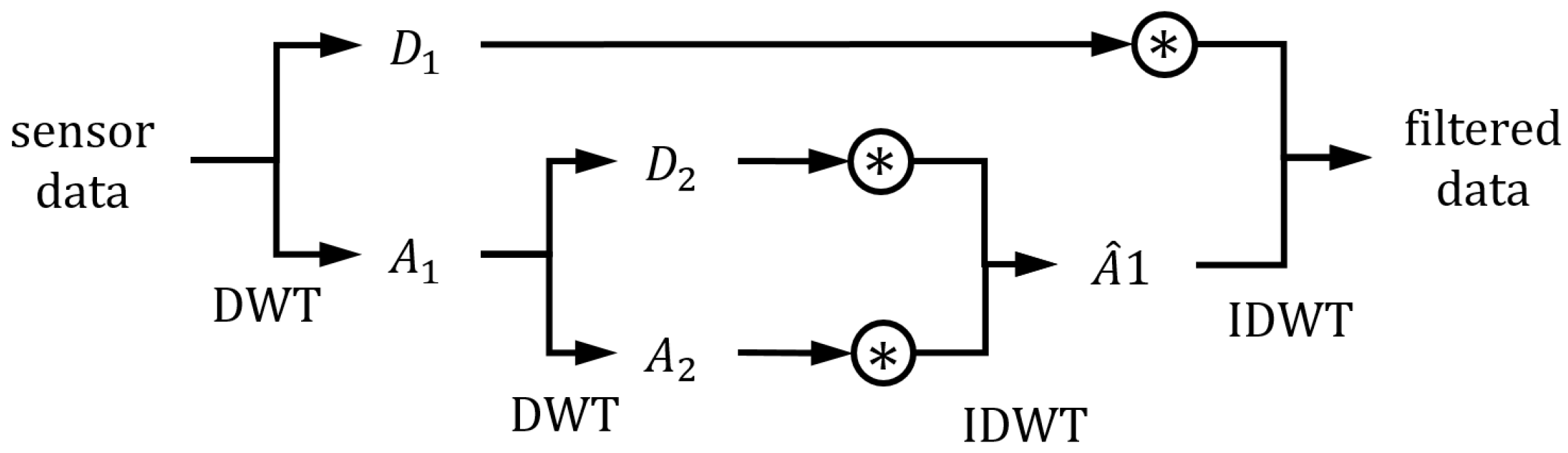
2.2. Wavelet Analysis
2.3. GAN
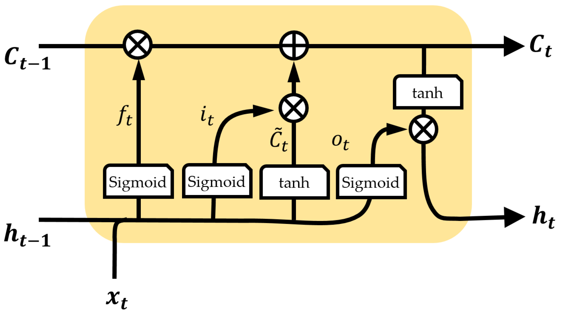
2.4. Long Short-Term Memory (LSTM)
3. Missile System and the Proposed Network
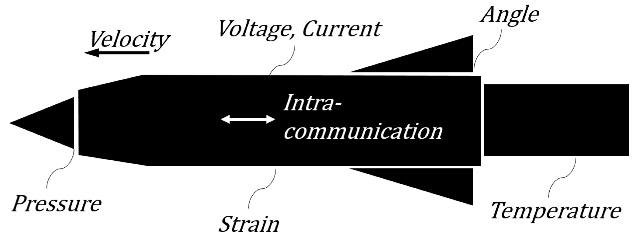
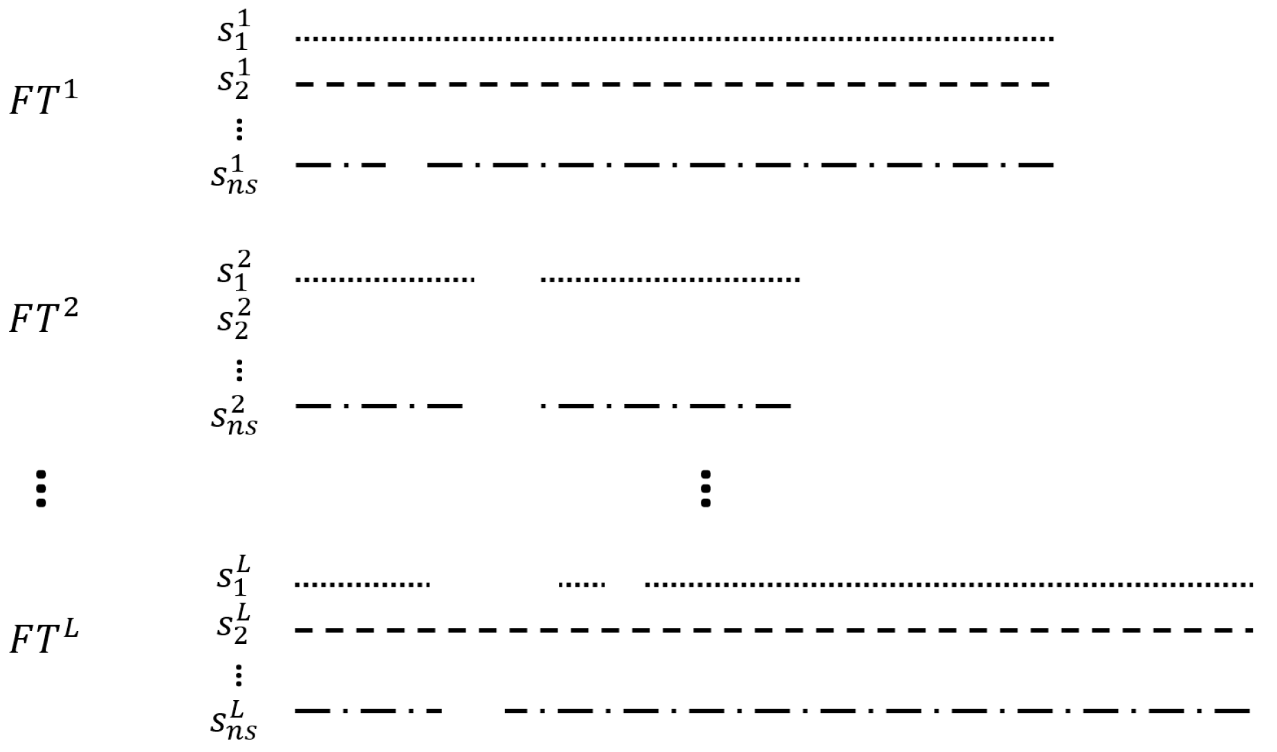
3.1. Missile Data
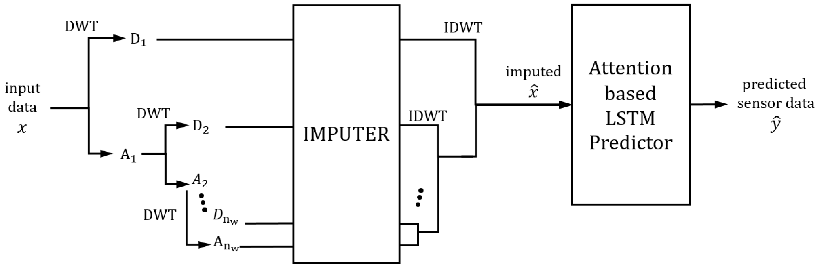
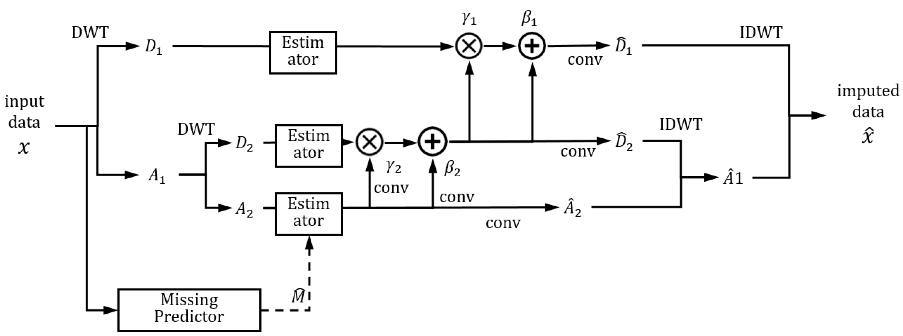
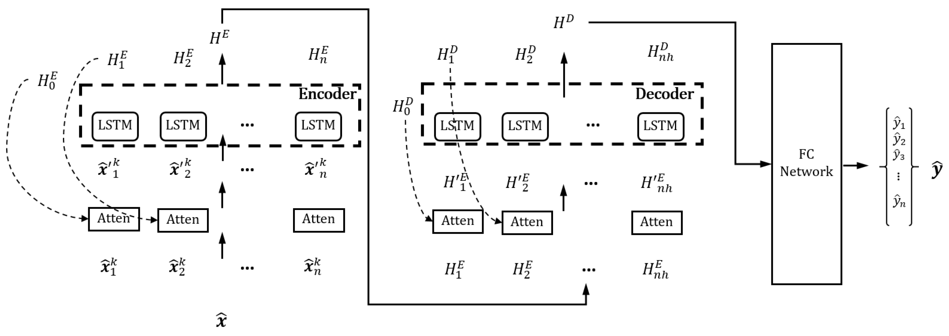
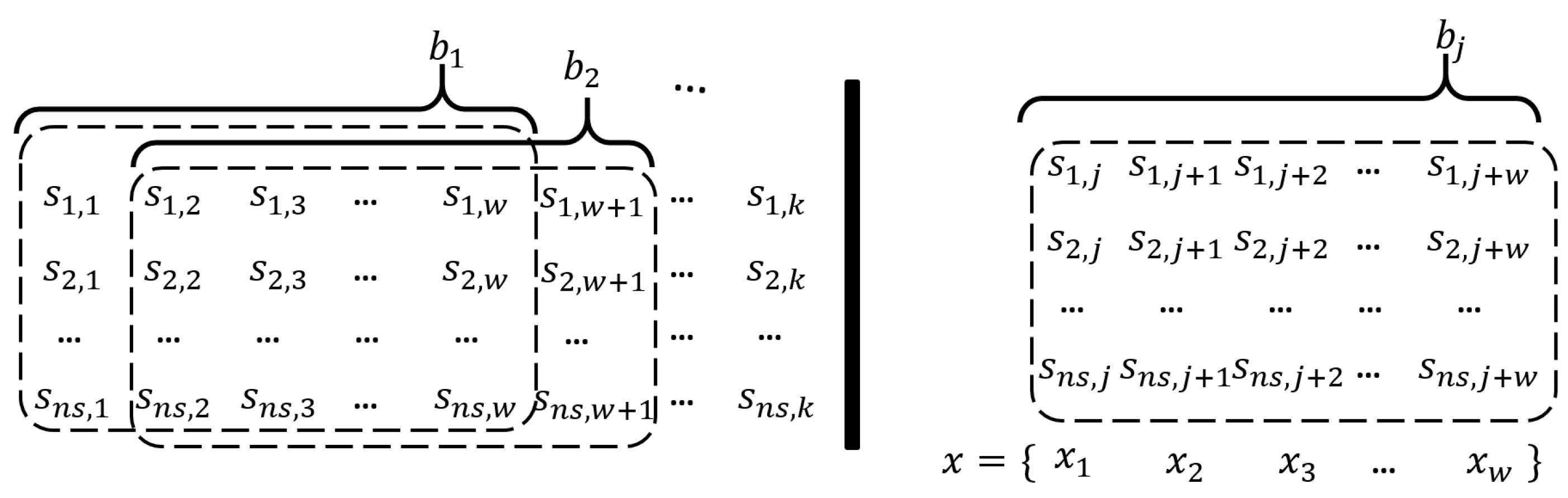
3.2. Network Architecture
3.3. Loss Function
4. Test Result
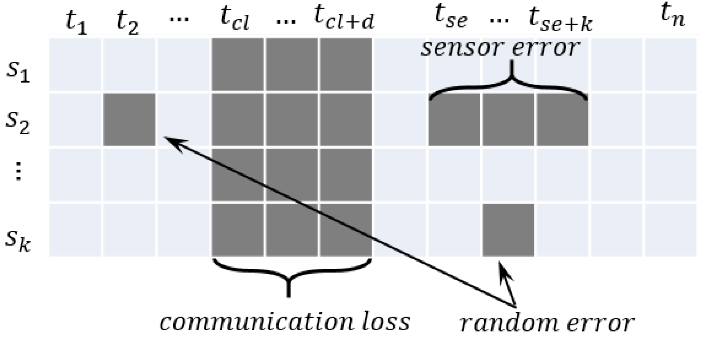
4.1. Test Setup
- 1.
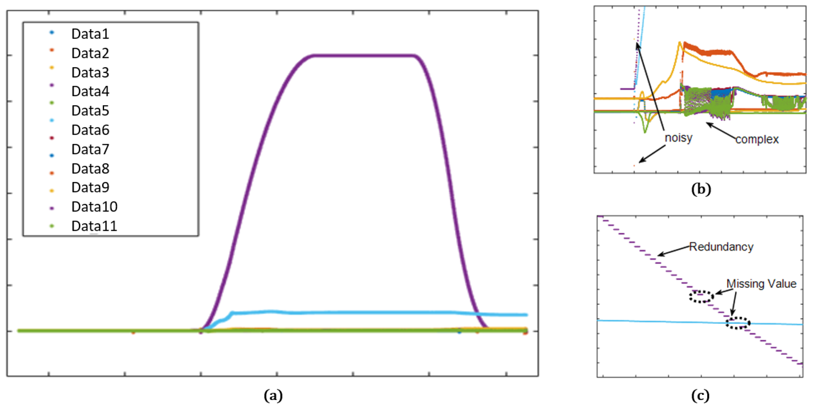
- Communication loss: Communication loss can occur at a random time for random time intervals, and all the data are lost. The missing values are generated at a random time () for random time intervals (f).
- 2.
- Sensor error: Sensor error can be caused by contact problems or corruption of sensors, and the specific sensor data are missing. The missing values are generated for the random sensor data for a random time () for random time intervals (k).
- 3.
- Random error: Random error can be caused by random noise or an unknown reason, and the missing values are generated for a random feature and random time.
4.2. Performance Evaluation
4.2.1. Quantitative Evaluation
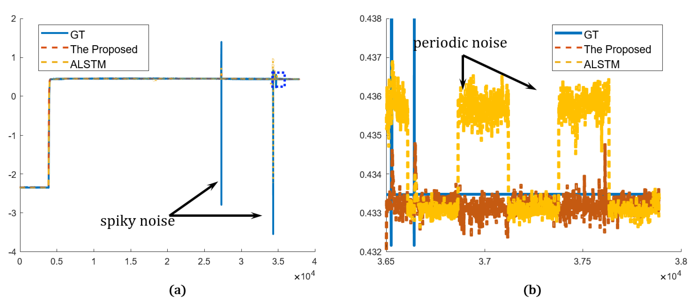
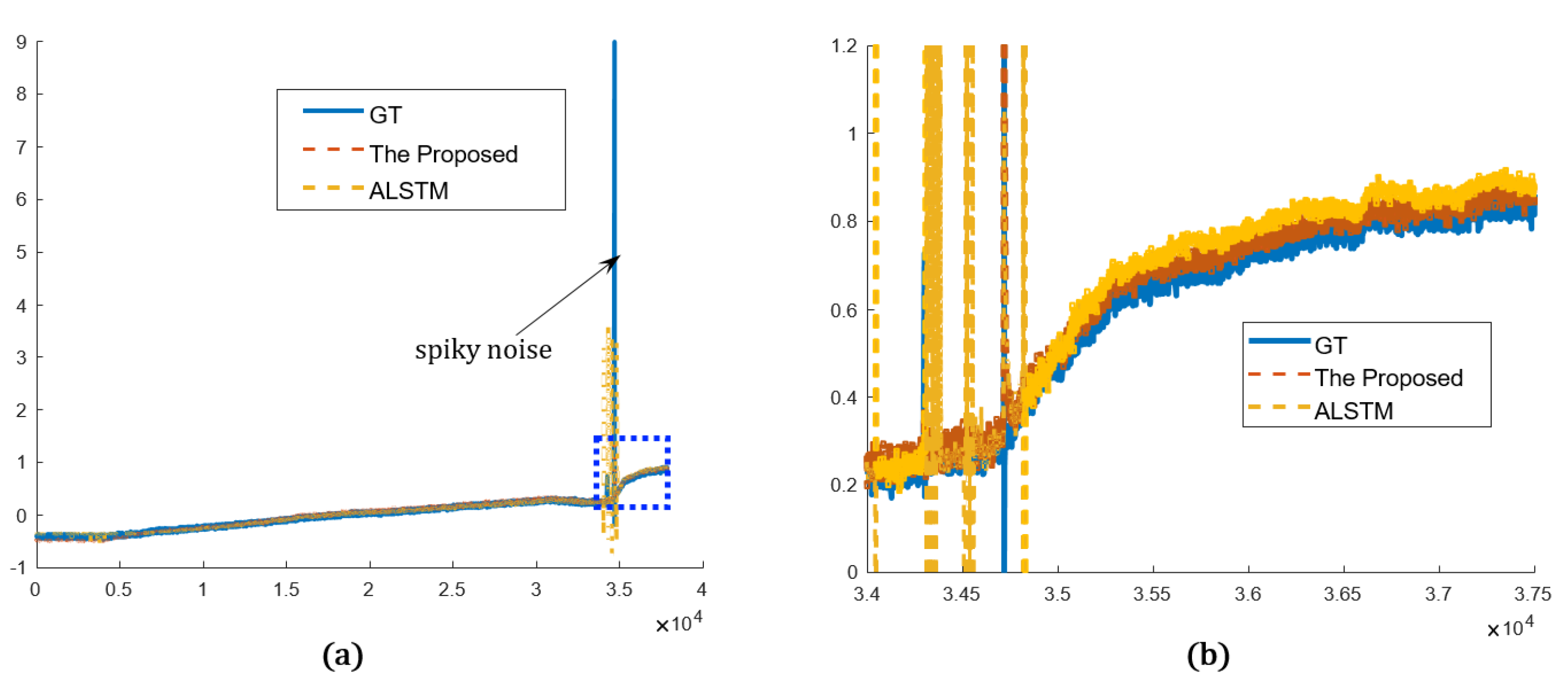
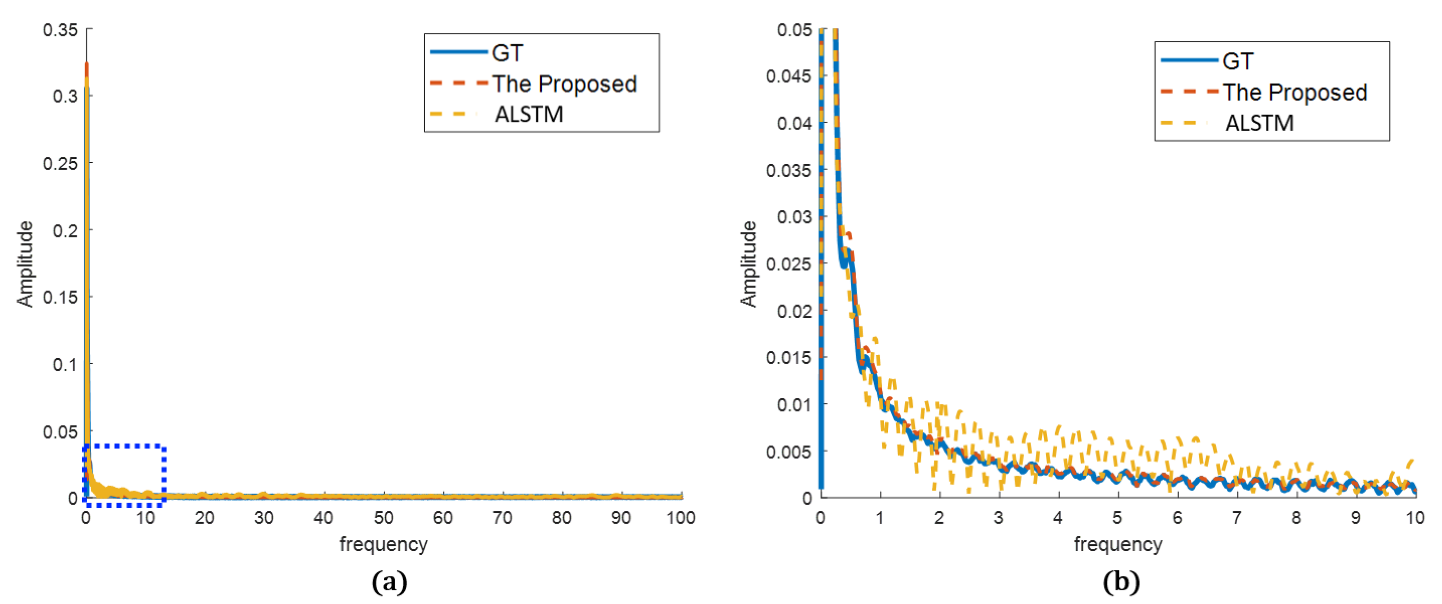
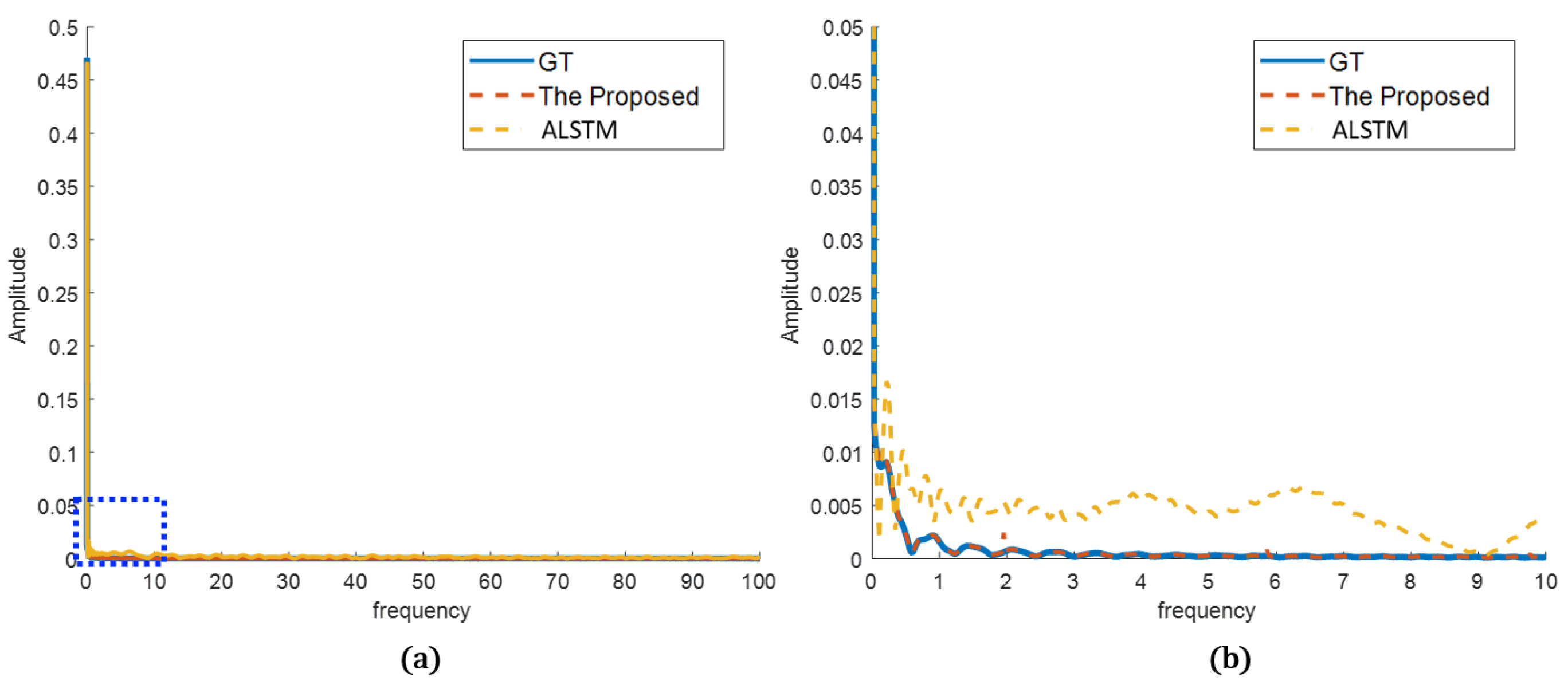
4.2.2. Qualitative Evaluation
5. Conclusions
Author Contributions
Funding
Institutional Review Board Statement
Data Availability Statement
Conflicts of Interest
References
- Leon-Medina, J.X.; Camacho, J.; Gutierrez-Osorio, C.; Salomón, J.E.; Rueda, B.; Vargas, W.; Sofrony, J.; Restrepo-Calle, F.; Tibaduiza, D.T. Temperature Prediction Using Multivariate Time Series Deep Learning in the Lining of an Electric Arc Furnace for Ferronickel Production. Sensors 2021, 21, 6894. [Google Scholar] [CrossRef] [PubMed]
- Macias, E.; Boquet, G.; Serrano, J.; Vicario, J.L.; Ibeas, J.; Morel, A. Novel imputing method and deep learning techniques for early prediction of sepsis in intensive care units. In Proceedings of the 2019 Computing in Cardiology, Singapore, 8–11 September 2019; pp. 1–4. [Google Scholar]
- Nikparvar, B.; Rahman, M.; Hatami, F.; Thill, J.C. Spatio-temporal prediction of the COVID-19 pandemic in US counties: Modeling with a deep LSTM neural network. Sci. Rep. 2021, 11, 21715. [Google Scholar] [CrossRef] [PubMed]
- Han, L.; Yu, C.; Xiao, K.; Zhao, X. A new method of mixed gas identification based on a convolutional neural network for time series classification. Sensors 2019, 19, 1960. [Google Scholar] [CrossRef] [PubMed]
- Li, Y.; Zhu, Z.; Kong, D.; Han, H.; Zhao, Y. EA-LSTM: Evolutionary attention-based LSTM for time series prediction. Knowl.-Based Syst. 2019, 19, 1960. [Google Scholar] [CrossRef]
- Rhif, M.; Ben Abbes, A.; Farah, I.R.; Martínez, B.; Sang, Y. Wavelet transform application for/in non-stationary time-series analysis: A review. Appl. Sci. 2019, 9, 1345. [Google Scholar] [CrossRef]
- Kim, T.; Ko, W.; Kim, J. Analysis and Impact Evaluation of Missing Data Imputation in Day-ahead PV Generation Forecasting. Appl. Sci. 2019, 9, 204. [Google Scholar] [CrossRef]
- Fu, Y.; He, H.S.; Hawbaker, T.J.; Henne, P.D.; Zhu, Z.; Larsen, D.R. Evaluating k-Nearest Neighbor (k NN) Imputation Models for Species-Level Aboveground Forest Biomass Mapping in Northeast China. Remote Sens. 2019, 11, 2005. [Google Scholar] [CrossRef]
- Valdiviezo, H.C.; Van Aelst, S. Tree-based prediction on incomplete data using imputation or surrogate decisions. J. Inf. Sci. 2015, 3131, 163–181. [Google Scholar] [CrossRef]
- Zhang, X.; Yan, C.; Gao, C.; Malin, B.; Chen, Y. XGBoost imputation for time series data. In Proceedings of the 2019 IEEE International Conference on Healthcare Informatics, Xi’an, China, 10–13 June 2019; pp. 1–3. [Google Scholar]
- Krithiga, R.; Ilavarasan, E. Hyperparameter tuning of AdaBoost algorithm for social spammer identification. Int. J. Pervasive Comput. Commun. 2021, 17, 462–482. [Google Scholar]
- Mikhchi, A.; Honarvar, M.; Kashan, N.E.J.; Zerehdaran, S.; Aminafshar, M. Analyses and comparison of K-nearest neighbour and AdaBoost algorithms for genotype imputation. Res. Vet. Sci. 2017, 5, 295–299. [Google Scholar]
- Lall, R.; Robinson, T. The MIDAS touch: Accurate and scalable missing-data imputation with deep learning. Political Anal. 2022, 30, 179–196. [Google Scholar] [CrossRef]
- Zhuang, Y.; Ke, R.; Wang, Y. Innovative method for traffic data imputation based on convolutional neural network. IET Intell. Transp. Syst. 2019, 13, 605–613. [Google Scholar] [CrossRef]
- Cao, W.; Wang, D.; Li, J.; Zhou, H.; Li, L.; Li, Y. Brits: Bidirectional recurrent imputation for time series. In Proceedings of the 32nd Conference on Neural Information Processing Systems (NeurIPS 2018), Montréal, QC, Canada, 2–8 December 2018; p. 31. [Google Scholar]
- Yoon, J.; Jordon, J.; Schaar, M. Gain: Missing data imputation using generative adversarial nets. In Proceedings of the 35th International Conference on Machine Learning, Stockholm, Sweden, 10–15 July 2018; pp. 5689–5698. [Google Scholar]
- Nibhanupudi, S.; Youssif, R.; Purdy, C. Data-specific signal denoising using wavelets, with applications to ECG data. In Proceedings of the 2004 47th Midwest Symposium on Circuits and Systems, Hiroshima, Japan, 25–28 July 2004; pp. 219–222. [Google Scholar]
- Joo, T.W.; Kim, S.B. Time series forecasting based on wavelet filtering. Expert Syst. Appl. 2015, 42, 3868–3874. [Google Scholar] [CrossRef]
- Ryu, S.; Koo, G.; Kim S., W. An Adaptive Selection of Filter Parameters: Defect Detection in Steel Image Using Wavelet Reconstruction Method. ISIJ Int. 2020, 60, 1703–1713. [Google Scholar] [CrossRef]
- Memarian S., O.; Asgari, J.; Amiri-Simkooei, A. Wavelet decomposition and deep learning of altimetry waveform retracking for Lake Urmia water level survey. Mar. Georesources Geotechnol. 2022, 40, 361–369. [Google Scholar] [CrossRef]
- Yu, Y.; Zhan, F.; Lu, S.; Pan, J.; Ma, F.; Xie, X.; Miao, C. Wavefill: A wavelet-based generation network for image inpainting. In Proceedings of the IEEE/CVF International Conference on Computer Vision, Montreal, QC, Canada, 11–17 October 2021; pp. 14114–14123. [Google Scholar]
- Guo, T.; Seyed Mousavi, H.; Huu Vu, T.; Monga, V. Deep wavelet prediction for image super-resolution. In Proceedings of the IEEE Conference on Computer Vision and Pattern Recognition Workshops, Honolulu, HI, USA, 21–26 July 2017; pp. 104–113. [Google Scholar]
- Sarhan, A.M. Brain tumor classification in magnetic resonance images using deep learning and wavelet transform. J. Biomed. Eng. 2020, 133, 102. [Google Scholar] [CrossRef]
- Goodfellow, I.; Pouget-Abadie, J.; Mirza, M.; Xu, B.; Warde-Farley, D.; Ozair, S.; Aaron, C.; Bengio, Y. Generative adversarial nets. Advances in neural information processing systems. Adv. Neural Inf. Process. Syst. 2014, 27. [Google Scholar]
- Xian, W.; Sangkloy, P.; Agrawal, V.; Raj, A.; Lu, J.; Fang, C.; Yu, F.; Hays, J. Texturegan: Controlling deep image synthesis with texture patches. In Proceedings of the IEEE Conference on Computer Vision and Pattern Recognition, Salt Lake City, UT, USA, 18–23 June 2018; pp. 8456–8465. [Google Scholar]
- Demir, U.; Unal, G. Patch-based image inpainting with generative adversarial networks. In Proceedings of the Conference on Computer Vision and Pattern Recognition, Salt Lake City, UT, USA, 18–23 June 2018. [Google Scholar]
- Zhang, W.; Li, X.; Jia, X.D.; Ma, H.; Luo, Z.; Li, X. Machinery fault diagnosis with imbalanced data using deep generative adversarial networks. Measurement 2020, 152, 107377. [Google Scholar] [CrossRef]
- Arjovsky, M.; Chintala, S.; Bottou, L. Wasserstein generative adversarial networks. In Proceedings of the International Conference on Machine Learning, Sydney, Australia, 6–11 August 2017; pp. 214–223. [Google Scholar]
- Saxena, D.; Cao, J. Generative adversarial networks (GANs) challenges, solutions, and future directions. ACM Comput. Surv. 2021, 54, 1–42. [Google Scholar] [CrossRef]
- Gulrajani, I.; Ahmed, F.; Arjovsky, M.; Dumoulin, V.; Courville, A.C. Improved training of wasserstein gans. Adv. Neural Inf. Process. Syst. 2017, 30. [Google Scholar]
- Connor, J.T.; Martin, R.D.; Atlas, L.E. Recurrent neural networks and robust time series prediction. IEEE Trans. Neural Netw. Learn. Syst. 1994, 5, 240–254. [Google Scholar] [CrossRef]
- Hochreiter, S.; Schmidhuber, J. Long short-term memory. Neural Comput. 1997, 9, 1735–1780. [Google Scholar] [CrossRef] [PubMed]
- Tiwari, G.; Sharma, A.; Sahotra, A.; Kapoor, R. English-Hindi neural machine translation-LSTM seq2seq and ConvS2S. In Proceedings of the 2020 International Conference on Communication and Signal Processing, Shanghai, China, 12–15 September 2020; pp. 871–875. [Google Scholar]
- Karim, F.; Majumdar, S.; Darabi, H.; Harford, S. Multivariate LSTM-FCNs for time series classification. Neural Netw. 2019, 116, 237–245. [Google Scholar] [CrossRef] [PubMed]
- Liu, X.; Lin, Z.; Feng, Z. Short-term offshore wind speed forecast by seasonal ARIMA-A comparison against GRU and LSTM. Energy 2021, 227, 120492. [Google Scholar] [CrossRef]
- Yamak, P.T.; Yujian, L.; Gadosey, P.K. A comparison between arima, lstm, and gru for time series forecasting. In Proceedings of the 2019 2nd International Conference on Algorithms, Computing and Artificial Intelligence, New York, NY, USA, 20–22 December 2019; pp. 49–55. [Google Scholar]
- Chung, J.; Gulcehre, C.; Cho, K.; Bengio, Y. Empirical evaluation of gated recurrent neural networks on sequence modeling. Neural and Evol. Comput. 2014, arXiv:1412.3555. [Google Scholar]
- Shewalkar, A. Performance evaluation of deep neural networks applied to speech recognition: RNN, LSTM and GRU. J. Artif. Intell. Soft Comput. Res. 2019, 9, 235–245. [Google Scholar] [CrossRef]
- Shewalkar, A.N. Comparison of rnn, lstm and gru on speech recognition data. Masters Thesis, North Dakota State University, Fargo, ND, USA, 2018. [Google Scholar]
- Yang, S.; Yu, X.; Zhou, Y. Lstm and gru neural network performance comparison study: Taking yelp review dataset as an example. In Proceedings of the 2020 International Workshop on Electronic Communication and Artificial Intelligence, Shanghai, China, 12–14 June 2020; pp. 98–101. [Google Scholar]
- Zarzycki, K.; Ławryńczuk, M. LSTM and GRU neural networks as models of dynamical processes used in predictive control: A comparison of models developed for two chemical reactors. Sensors 2021, 21, 5625. [Google Scholar] [CrossRef]
- Zhan, H.; Weerasekera, C.S.; Bian, J.W.; Reid, I. Visual odometry revisited: What should be learnt? In Proceedings of the 2020 IEEE International Conference on Robotics and Automation, Virtual Conference, 1 June–31 August 2020; pp. 4203–4210. [Google Scholar]
- Qin, Y.; Song, D.; Chen, H.; Cheng, W.; Jiang, G.; Cottrell, G. A dual-stage attention-based recurrent neural network for time series prediction. Mach. Learn. 2017, arXiv:1704.02971. [Google Scholar]


| Advantage | Disadvantage | ||
|---|---|---|---|
| Test-based modelling |
|
| |
|
Data driven | Traditional (ARMA, ARIMA) |
|
|
| Deep learning -based method |
|
| |
| Time | Data1 | Data2 | Data3 | Data4 | Data5 | Data6 | Data7 | Data8 | Data9 | Data10 | Data11 |
|---|---|---|---|---|---|---|---|---|---|---|---|
| 50.433 s | 0.9940 | 2.7940 | 0.9830 | 10,070 | −1.423 | 827.42 | 23.816 | 22.346 | NaN | 41.806 | 24.032 |
| 50.437 s | NaN | NaN | NaN | NaN | NaN | NaN | NaN | NaN | 45.2868 | NaN | NaN |
| 50.438 s | 0.9940 | 2.7940 | 0.9830 | 10,070 | −1.423 | 827.42 | 23.780 | 23.346 | NaN | 41.792 | 24 |
| 50.442 s | NaN | NaN | NaN | NaN | NaN | NaN | NaN | NaN | 45.2868 | NaN | NaN |
| 50.443 s | 0.9940 | 2.7940 | 0.9830 | 10,070 | −1.423 | 827.42 | 23.780 | 22.325 | NaN | 41.792 | 24 |
| 50.447 s | NaN | NaN | NaN | NaN | NaN | NaN | NaN | NaN | 45.0913 | NaN | NaN |
| 50.448 s | 0.9940 | 2.7940 | 0.9830 | 10,070 | −1.423 | 827.42 | 23.754 | 22.325 | NaN | 41.758 | 23.983 |
| 50.452 s | NaN | NaN | NaN | NaN | NaN | NaN | NaN | NaN | 45.2868 | NaN | NaN |
| 50.453 s | 0.9940 | 2.7930 | 0.9830 | 10,070 | −1.423 | 827.42 | 23.754 | 22.308 | NaN | 41.758 | 23.983 |
| 50.457 s | NaN | NaN | NaN | NaN | NaN | NaN | NaN | NaN | 45.2868 | NaN | NaN |
| 50.458 s | 0.9940 | 2.7930 | 0.9830 | 10,070 | −1.423 | 827.42 | 23.733 | 22.308 | NaN | 41.734 | 23.974 |
| 50.462 s | NaN | NaN | NaN | NaN | NaN | NaN | NaN | NaN | 45.6778 | NaN | NaN |
| 50.463 s | 1 | 2.7930 | 0.9830 | 10,070 | −1.423 | 826.91 | 23.733 | 22.284 | NaN | 41.734 | 23.974 |
| 50.467 s | NaN | NaN | NaN | NaN | NaN | NaN | NaN | NaN | 45.0913 | NaN | NaN |
| 50.468 s | 1 | 2.7930 | 0.9830 | 10,082 | −1.423 | 826.91 | 23.716 | 22.284 | NaN | 41.711 | 23.923 |
| Model | Parameters |
|---|---|
| No. iterations | 200 |
| Learning rate | 0.001 |
| Optimizer | Adam optimizer |
| Batch size | 512 |
| Window size | 128 |
| No. LSTM layer | 2 |
| No. hidden layer | 64 |
| Dropout in LSTM | 0.4 |
| Model | MAE | MSE | RMSE | MAPE |
|---|---|---|---|---|
| Basic LSTM | 0.454 | 0.555 | 0.676 | 5.184 |
| WLSTM | 0.075 | 0.022 | 0.126 | 1.290 |
| ALSTM | 0.041 | 0.073 | 0.215 | 0.951 |
| Proposed Method | 0.035 | 0.014 | 0.077 | 0.489 |
| Model | Missing Rate | ||||
|---|---|---|---|---|---|
| 1.15% | 2.3% | 4.6% | 9% | 17% | |
| WLSTM | 0.067 | 0.071 | 0.066 | 0.081 | 0.099 |
| 0.022 | 0.023 | 0.023 | 0.029 | 0.041 | |
| 0.127 | 0.133 | 0.128 | 0.147 | 0.179 | |
| ALSTM | 0.045 | 0.049 | 0.056 | 0.070 | 0.097 |
| 0.081 | 0.078 | 0.071 | 0.081 | 0.088 | |
| 0.226 | 0.227 | 0.227 | 0.241 | 0.263 | |
| Proposed Method | 0.037 | 0.039 | 0.044 | 0.053 | 0.070 |
| 0.016 | 0.017 | 0.021 | 0.025 | 0.039 | |
| 0.091 | 0.097 | 0.115 | 0.129 | 0.163 | |
Publisher’s Note: MDPI stays neutral with regard to jurisdictional claims in published maps and institutional affiliations. |
© 2022 by the authors. Licensee MDPI, Basel, Switzerland. This article is an open access article distributed under the terms and conditions of the Creative Commons Attribution (CC BY) license (https://creativecommons.org/licenses/by/4.0/).
Share and Cite
Ryu, S.-G.; Jeong, J.J.; Shim, D.H. Sensor Data Prediction in Missile Flight Tests. Sensors 2022, 22, 9410. https://doi.org/10.3390/s22239410
Ryu S-G, Jeong JJ, Shim DH. Sensor Data Prediction in Missile Flight Tests. Sensors. 2022; 22(23):9410. https://doi.org/10.3390/s22239410
Chicago/Turabian StyleRyu, Sang-Gyu, Jae Jin Jeong, and David Hyunchul Shim. 2022. "Sensor Data Prediction in Missile Flight Tests" Sensors 22, no. 23: 9410. https://doi.org/10.3390/s22239410
APA StyleRyu, S.-G., Jeong, J. J., & Shim, D. H. (2022). Sensor Data Prediction in Missile Flight Tests. Sensors, 22(23), 9410. https://doi.org/10.3390/s22239410