
A Novel Joint Adversarial Domain Adaptation Method for Rotary Machine Fault Diagnosis under Different Working Conditions


Abstract
1. Introduction
2. Preliminaries
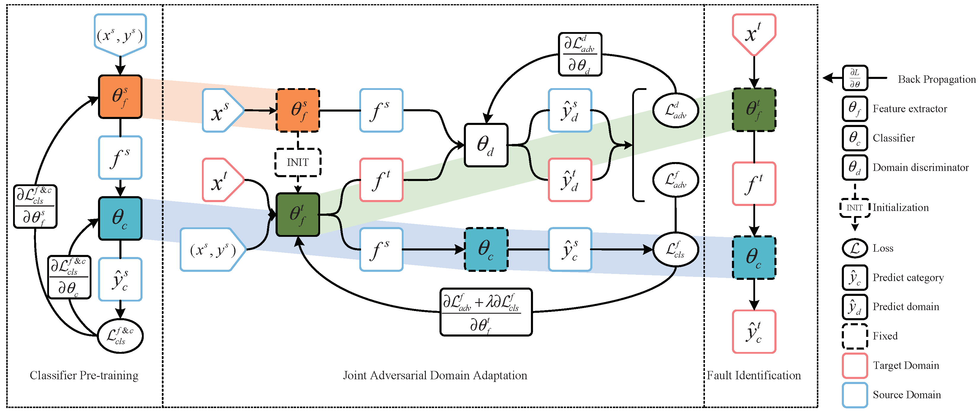
3. The Proposed Method
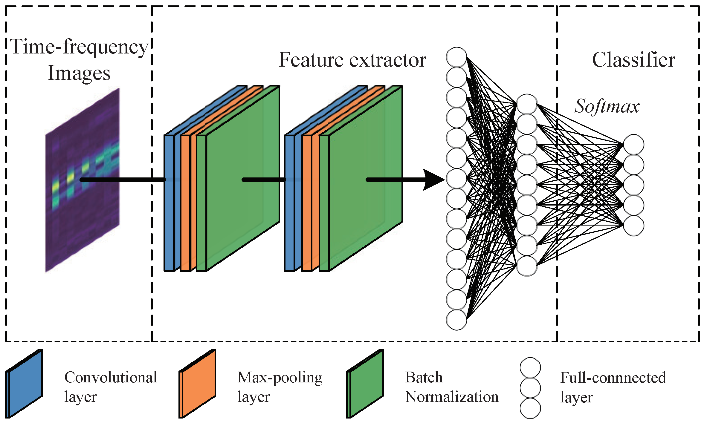
3.1. Classifier Pre-Training
3.2. Joint Adversarial Domain Adaptation
3.3. Fault Identification
4. Experiment and Result Analysis
4.1. Experiments on DDS Dataset
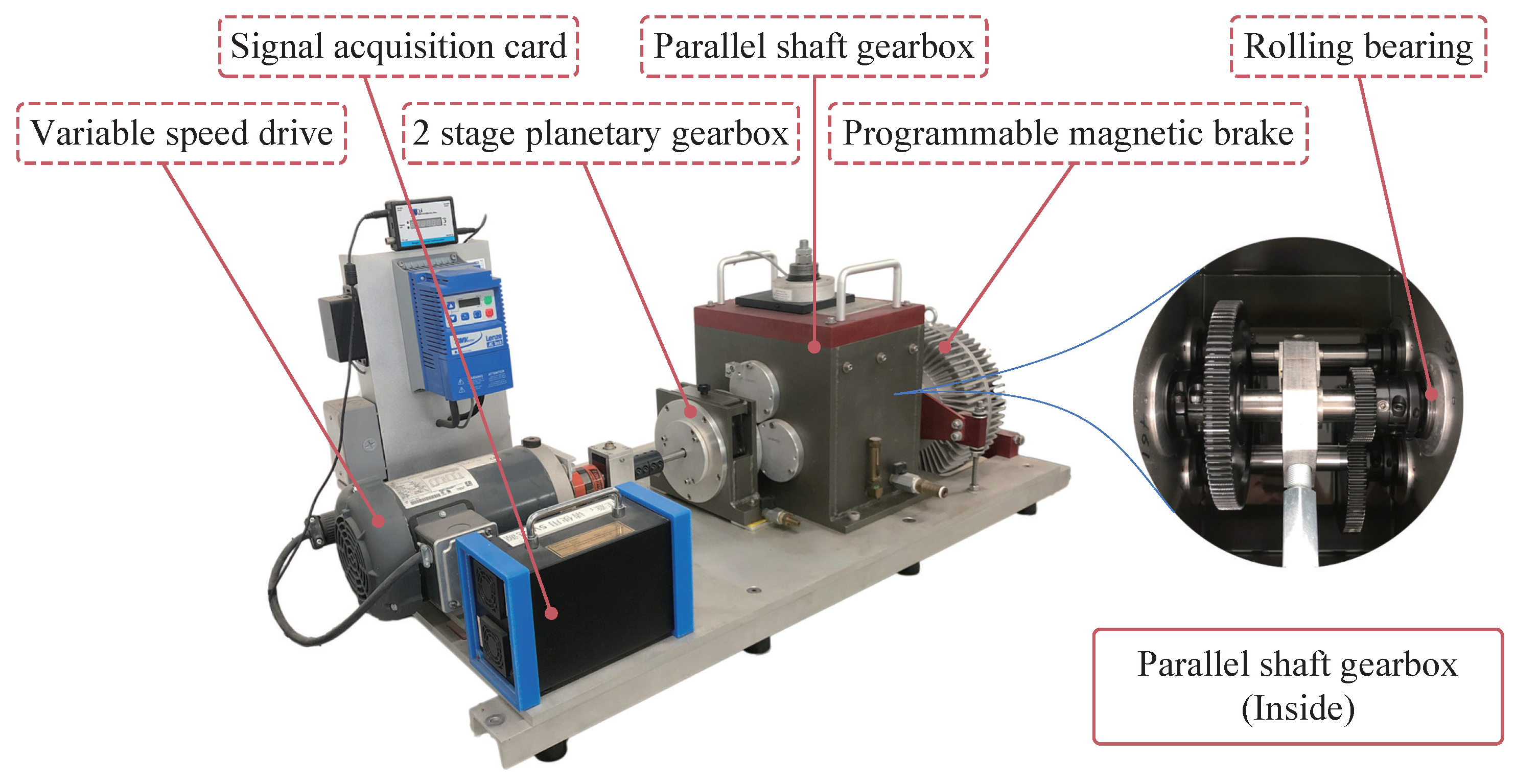
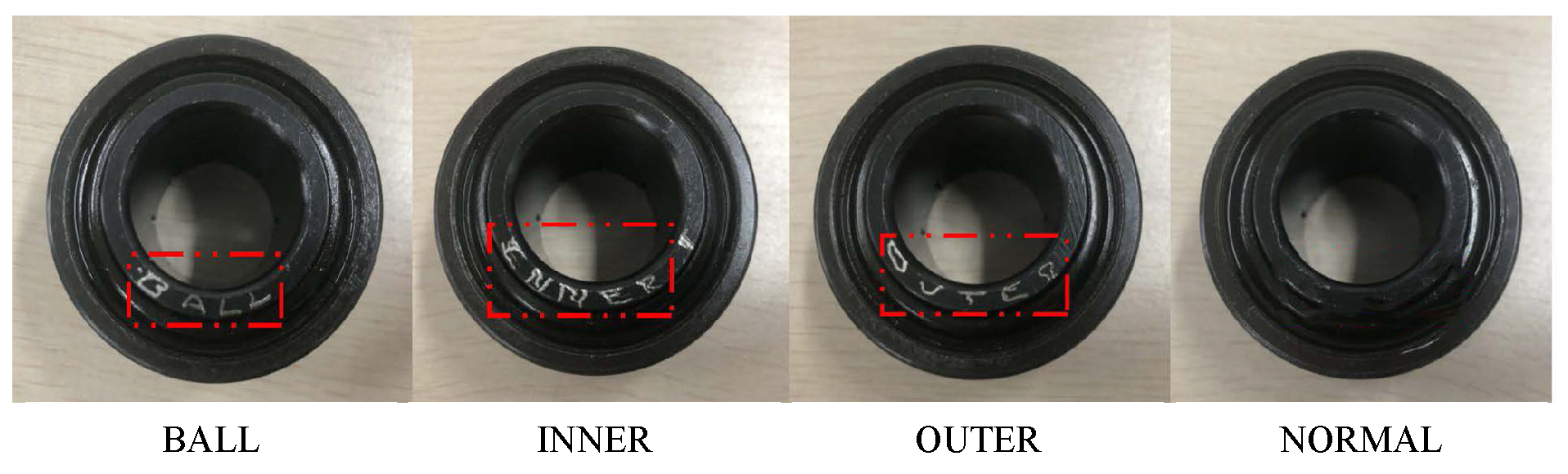
4.1.1. Data Description
4.1.2. Transfer Diagnosis Tasks Settings
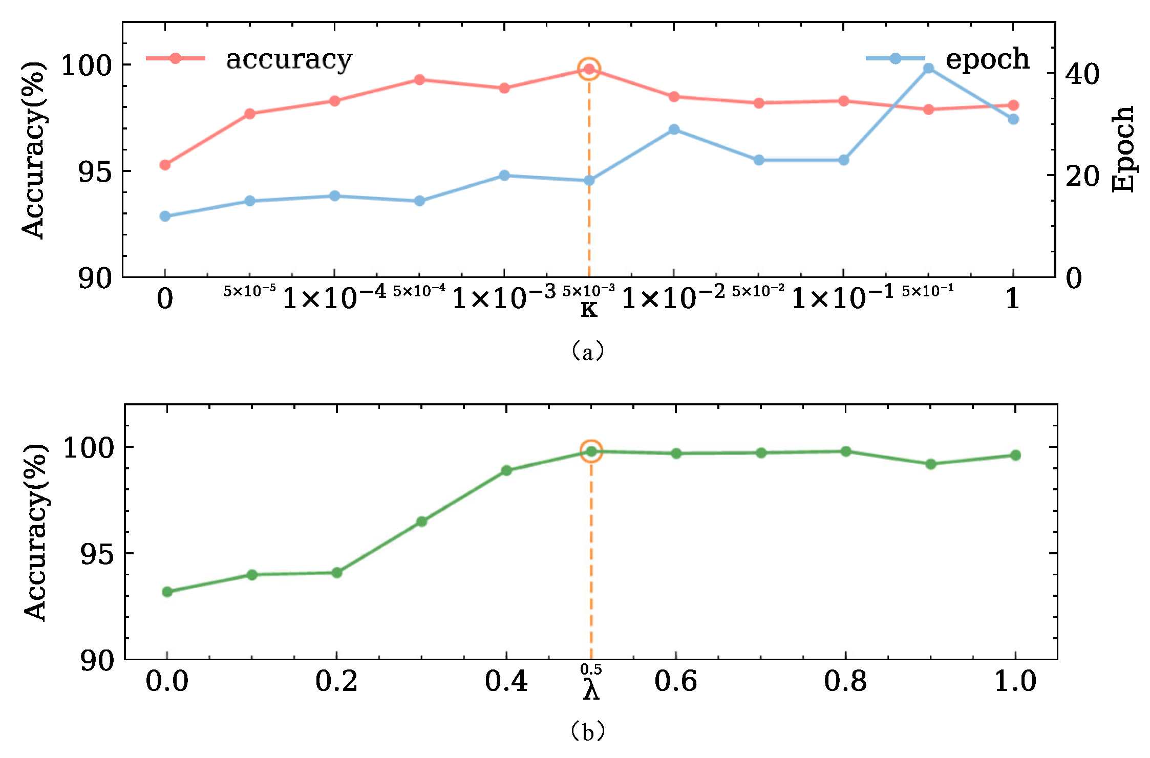
4.1.3. Parameters of the Proposed Method
4.1.4. Comparison Methods
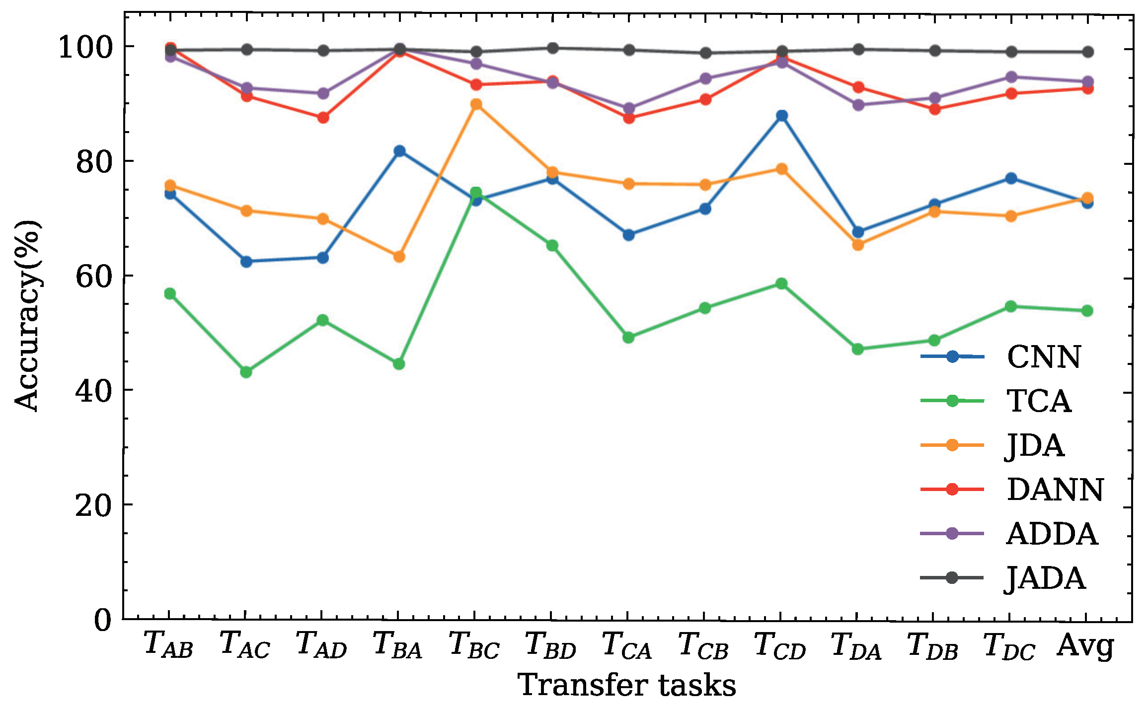
4.1.5. Result Analysis
4.2. Experiments on the CWRU Dataset
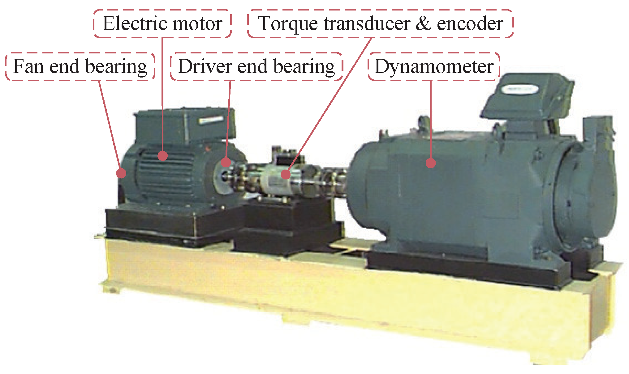
4.2.1. Data Descriptions
4.2.2. Transfer Diagnosis Tasks Settings
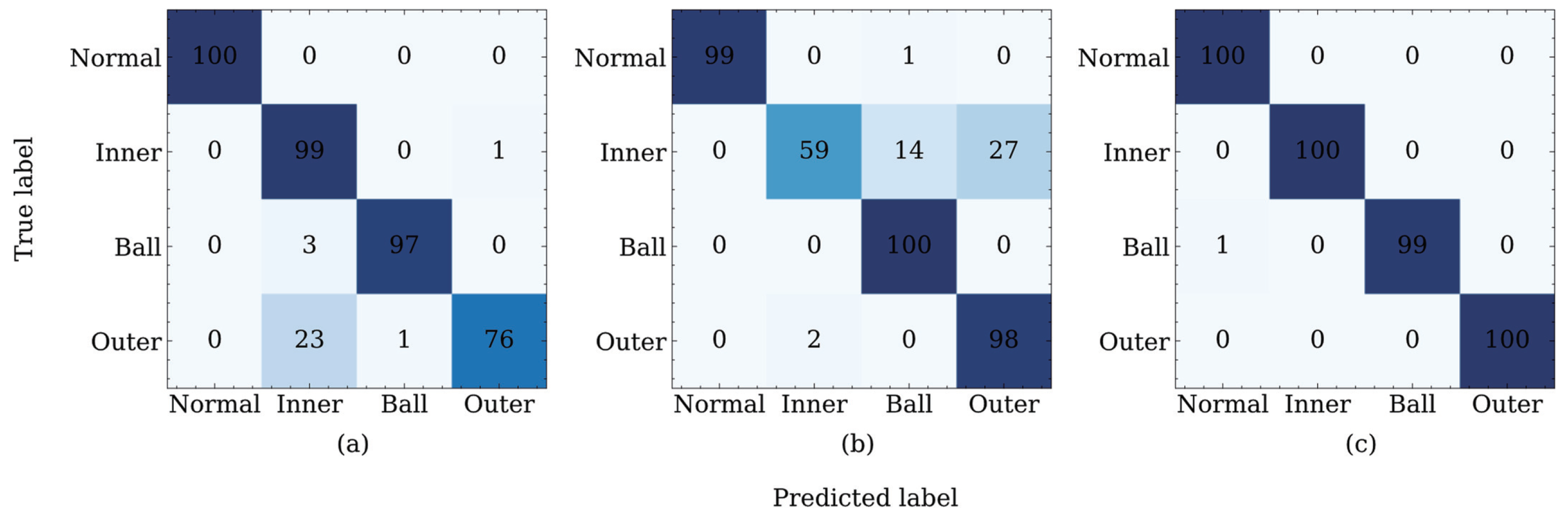
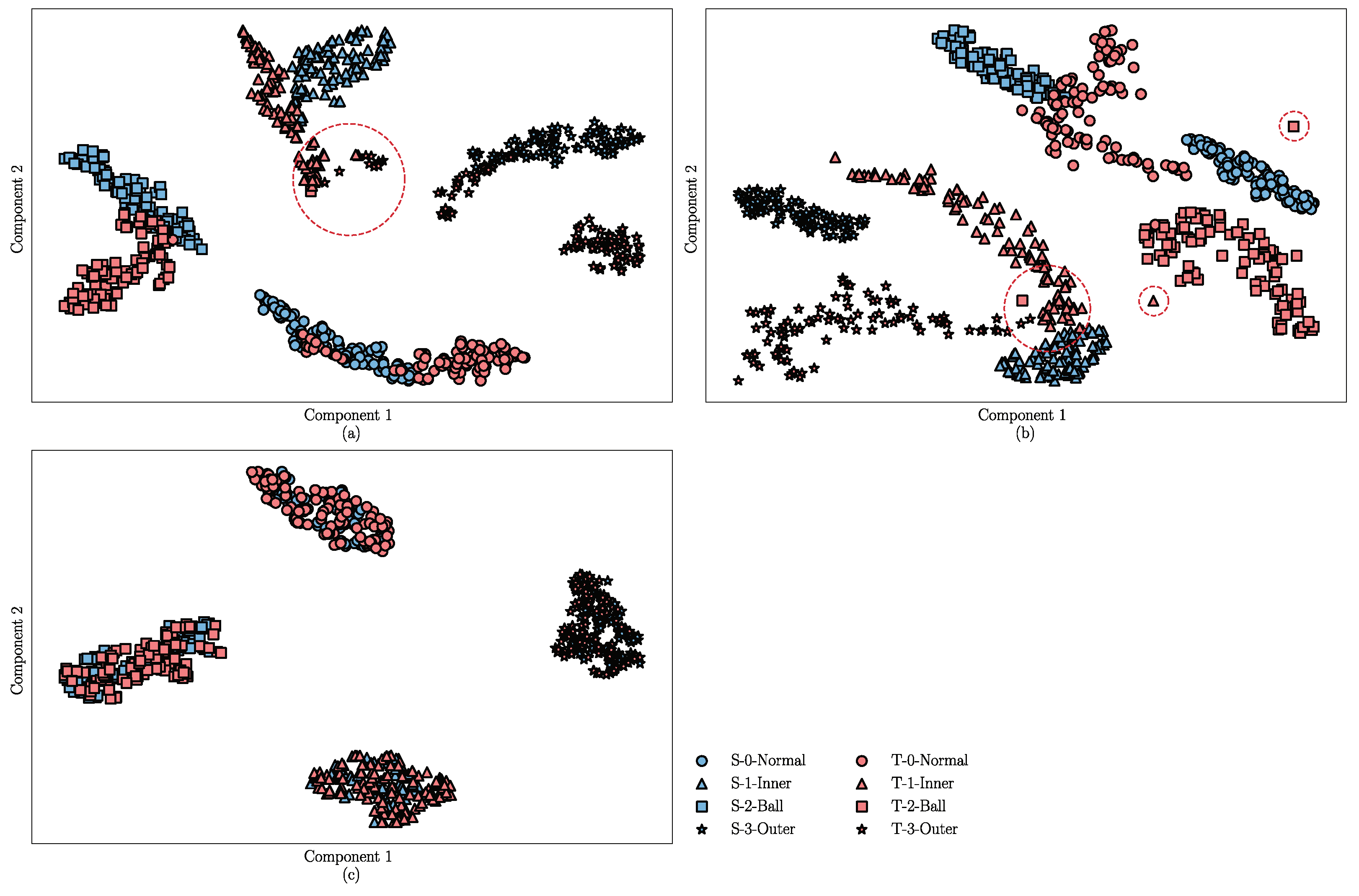
4.2.3. Result Analysis
5. Conclusions
Author Contributions
Funding
Institutional Review Board Statement
Informed Consent Statement
Data Availability Statement
Conflicts of Interest
References
- Zhou, Y.; Kumar, A.; Parkash, C. A novel entropy-based sparsity measure for prognosis of bearing defects and development of a sparsogram to select sensitive filtering band of an axial piston pump. Measurement 2022, 203, 111997. [Google Scholar] [CrossRef]
- Chen, Z.; Mauricio, A.; Li, W. A deep learning method for bearing fault diagnosis based on cyclic spectral coherence and convolutional neural networks. Mech. Syst. Sig. Process. 2020, 140, 106683. [Google Scholar] [CrossRef]
- Zhao, R.; Yan, R.; Chen, Z. Deep learning and its applications to machine health monitoring. Mech. Syst. Sig. Process. 2019, 115, 213–237. [Google Scholar] [CrossRef]
- Zhu, J.; Chen, N.; Peng, W. Estimation of bearing remaining useful life based on multiscale convolutional neural network. IEEE Trans. Ind. Electron. 2018, 66, 3208–3216. [Google Scholar] [CrossRef]
- Shao, H.; Jiang, H.; Zhao, H. A novel deep autoencoder feature learning method for rotating machinery fault diagnosis. Mech. Syst. Sig. Process. 2017, 95, 187–204. [Google Scholar] [CrossRef]
- Yang, B.; Lei, Y.; Jia, F. An intelligent fault diagnosis approach based on transfer learning from laboratory bearings to locomotive bearings. Mech. Syst. Sig. Process. 2019, 122, 692–706. [Google Scholar] [CrossRef]
- Jiao, J.; Zhao, M.; Lin, J. Residual joint adaptation adversarial network for intelligent transfer fault diagnosis. Mech. Syst. Sig. Process. 2020, 145, 106962. [Google Scholar] [CrossRef]
- Shao, H.; Xia, M.; Han, G. Intelligent fault diagnosis of rotor-bearing system under varying working conditions with modified transfer convolutional neural network and thermal images. IEEE Trans. Ind. Inf. 2020, 17, 3488–3496. [Google Scholar] [CrossRef]
- Zhou, Y.; Zhi, G.; Chen, W. A new tool wear condition monitoring method based on deep learning under small samples. Measurement 2022, 189, 110622. [Google Scholar] [CrossRef]
- Yosinski, J.; Clune, J.; Bengio, Y. How transferable are features in deep neural networks? Adv. Neural Inf. Process. Syst. 2014, 27, 3320–3328. [Google Scholar]
- Shao, S.; McAleer, S.; Yan, R. Highly accurate machine fault diagnosis using deep transfer learning. IEEE Trans. Ind. Inf. 2018, 15, 2446–2455. [Google Scholar] [CrossRef]
- Cao, P.; Zhang, S.; Tang, J. Preprocessing-free gear fault diagnosis using small datasets with deep convolutional neural network-based transfer learning. IEEE Access 2018, 6, 26241–26253. [Google Scholar] [CrossRef]
- Zhang, B.; Li, W.; Li, L. Intelligent fault diagnosis under varying working conditions based on domain adaptive convolutional neural networks. IEEE Access 2018, 6, 66367–66384. [Google Scholar] [CrossRef]
- Zhao, K.; Jiang, H.; Wang, K. Joint distribution adaptation network with adversarial learning for rolling bearing fault diagnosis. Knowl.-Based Syst. 2021, 222, 106974. [Google Scholar] [CrossRef]
- Zhao, B.; Zhang, X.; Zhan, Z. Deep multi-scale adversarial network with attention: A novel domain adaptation method for intelligent fault diagnosis. J. Manuf. Syst. 2021, 59, 565–576. [Google Scholar] [CrossRef]
- Lu, W.; Liang, B.; Cheng, Y. Deep model based domain adaptation for fault diagnosis. IEEE Trans. Ind. Electron. 2016, 64, 2296–2305. [Google Scholar] [CrossRef]
- Lei, Y.; Yang, B.; Du, Z. Deep Transfer Diagnosis Method for Machinery in Big Data Era. J. Mech. Eng. 2019, 55, 1–8. [Google Scholar] [CrossRef]
- Guo, L.; Lei, Y.; Xing, S. Deep convolutional transfer learning network: A new method for intelligent fault diagnosis of machines with unlabeled data. IEEE Trans. Ind. Electron. 2018, 66, 7316–7325. [Google Scholar] [CrossRef]
- Wen, L.; Gao, L.; Li, X. A new deep transfer learning based on sparse auto-encoder for fault diagnosis. IEEE Trans. Syst. Man Cybern. Syst. 2017, 49, 136–144. [Google Scholar] [CrossRef]
- Chen, C.; Li, Z.; Yang, J. A cross domain feature extraction method based on transfer component analysis for rolling bearing fault diagnosis. In Proceedings of the 29th Chinese Control Furthermore, Decision Conference (CCDC), ChongQing, China, 28 May 2017; pp. 5622–5626. [Google Scholar]
- Wu, Z.; Jiang, H.; Zhao, K. An adaptive deep transfer learning method for bearing fault diagnosis. Measurement 2020, 151, 107227. [Google Scholar] [CrossRef]
- Saito, K.; Watanabe, K.; Ushiku, Y. Maximum classifier discrepancy for unsupervised domain adaptation. In Proceedings of the IEEE Conference on Computer Vision and Pattern Recognition, Salt Lake City, UT, USA, 18–22 June 2018; pp. 3723–3732. [Google Scholar]
- Wen, Y.; Zhang, K.; Li, Z. A discriminative feature learning approach for deep face recognition. In Proceedings of the European Conference on Computer Vision, Amsterdam, The Netherlands, 8–16 October 2016; pp. 499–515. [Google Scholar]
- Li, S.; Liu, C.; Xie, B. Joint adversarial domain adaptation. In Proceedings of the 27th ACM International Conference on Multimedia, Nice, France, 21–25 October 2019; pp. 729–737. [Google Scholar]
- The Case Western Reserve University Bearing Data Center Website. Available online: https://engineering.case.edu/bearingdatacenter (accessed on 31 January 2002).
- Pan, S.; Tsang, I.; Kwok, J. Domain adaptation via transfer component analysis. IEEE Trans. Neural Net. 2010, 22, 199–210. [Google Scholar] [CrossRef] [PubMed]
- Long, M.; Wang, J.; Ding, G. Transfer feature learning with joint distribution adaptation. In Proceedings of the IEEE International Conference on Computer Vision, Sydney, NSW, Australia, 1–8 December 2013; pp. 2200–2207. [Google Scholar]
- Ganin, Y.; Lempitsky, V. Unsupervised domain adaptation by backpropagation. In Proceedings of the International Conference on Machine Learning, Lile, France, 6–11 July 2015; pp. 1180–1189. [Google Scholar]
- Tzeng, E.; Hoffman, J.; Saenko, K. Adversarial discriminative domain adaptation. In Proceedings of the IEEE Conference on Computer Vision and Pattern Recognition, Honolulu, HI, USA, 22–25 July 2017; pp. 7167–7176. [Google Scholar]
- Sun, C.; Ma, M.; Zhao, Z. Sparse deep stacking network for fault diagnosis of motor. IEEE Trans. Ind. Inf. 2018, 14, 3261–3270. [Google Scholar] [CrossRef]
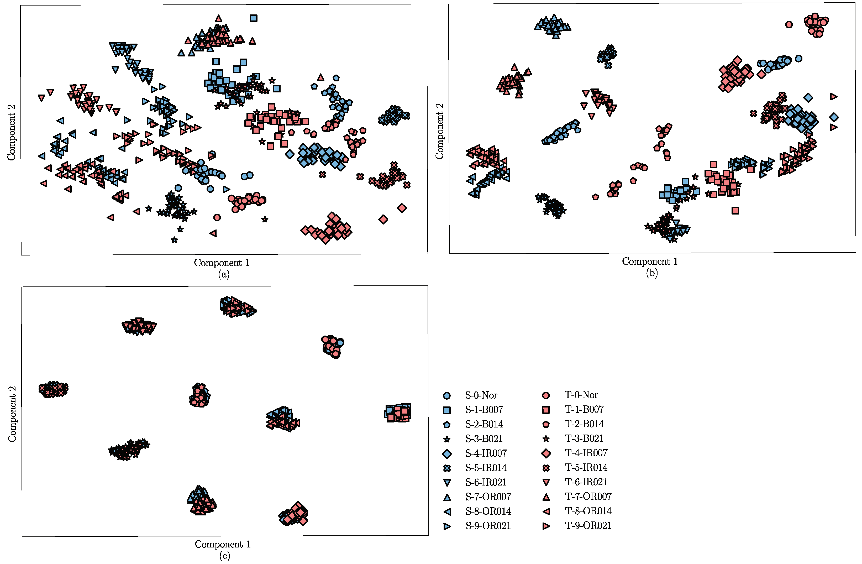
- Maaten, L.; Hinton, G. Visualizing data using t-SNE. J. Mach. Learn 2008, 9, 2579–2605. [Google Scholar]
- Shao, J.; Huang, Z.; Zhu, J. Transfer learning method based on adversarial domain adaption for bearing fault diagnosis. IEEE Access 2020, 8, 119421–119430. [Google Scholar] [CrossRef]


| Fault Class | Domain | |||
|---|---|---|---|---|
| A(0V) | B(4V) | C(6V) | D(8V) | |
| Normal | Normal_0 | Normal_4 | Normal_4 | Normal_4 |
| Inner race | Inner_0 | Inner_4 | Inner_4 | Inner_4 |
| Ball | Ball_0 | Ball_4 | Ball_4 | Ball_4 |
| Outer race | Outer_0 | Outer_4 | Outer_4 | Outer_4 |
| Transfer Tasks | ||||||||||||
|---|---|---|---|---|---|---|---|---|---|---|---|---|
| Source domain | A | A | A | B | B | B | C | C | C | D | D | D |
| Target domain | B | C | D | A | C | D | A | B | D | A | B | C |
| Module | Layer Type | Activation Function | Kernel Size | Stride | Output Size |
|---|---|---|---|---|---|
| Feature extractor | Conv_1 | relu | 3 × 3 | 1 | (64, 64, 16) |
| Batch Norm | / | / | / | (64, 64, 16) | |
| Max-pooling | / | 3 × 3 | 2 | (32, 32, 16) | |
| Conv_2 | relu | 3 × 3 | 1 | (32, 32, 64) | |
| Batch Norm | / | / | / | (32, 32, 64) | |
| Max-pooling | / | 3 × 3 | 2 | (16, 16, 64) | |
| Flatten | / | / | / | (1, 16 × 16 × 64) | |
| FC_1 | relu | / | / | (1, 256) | |
| FC_2 | tanh | / | / | (1, 128) | |
| Classifier | FC_3 | softmax | / | / | (1, 4) |
| Discriminator | FC_4 | Leaky Relu | / | / | (1, 128) |
| FC_5 | Leaky Relu | / | / | (1, 128) | |
| FC_6 | sigmoid | / | / | (1, 1) |
| Method | Avg | ||||||||||||
|---|---|---|---|---|---|---|---|---|---|---|---|---|---|
| CNN | 74.32 | 62.45 | 63.19 | 81.87 | 73.29 | 77.11 | 67.32 | 71.93 | 88.26 | 67.95 | 72.80 | 77.41 | 73.16 |
| TCA | 56.87 | 43.20 | 52.31 | 44.70 | 74.73 | 65.47 | 49.43 | 54.62 | 58.93 | 47.52 | 49.10 | 55.06 | 54.33 |
| JDA | 75.76 | 71.38 | 70.02 | 63.48 | 90.10 | 78.25 | 76.28 | 76.16 | 78.97 | 65.76 | 71.59 | 70.85 | 74.05 |
| DANN | 99.76 | 91.38 | 87.66 | 99.23 | 93.48 | 94.11 | 87.74 | 91.03 | 98.42 | 93.23 | 89.45 | 92.21 | 93.14 |
| ADDA | 98.25 | 92.82 | 91.92 | 99.73 | 97.16 | 93.87 | 89.49 | 94.70 | 97.53 | 90.18 | 91.44 | 95.13 | 94.35 |
| JADA | 99.35 | 99.50 | 99.35 | 99.61 | 99.23 | 99.92 | 99.61 | 99.13 | 99.47 | 99.84 | 99.65 | 99.49 | 99.51 |
| Fault Locations | Motor Loads | |||
|---|---|---|---|---|
| 0 hp | 1 hp | 2 hp | 3 hp | |
| Normal | Nor_0 | Nor_1 | Nor_2 | Nor_3 |
| IR | IR007_0 | IR007_1 | IR007_2 | IR007_3 |
| IR014_0 | IR014_1 | IR014_2 | IR014_3 | |
| IR021_0 | IR021_1 | IR021_2 | IR021_3 | |
| B | B007_0 | B007_1 | B007_2 | B007_3 |
| B014_0 | B014_1 | B014_2 | B014_3 | |
| B021_0 | B021_1 | B021_2 | B021_3 | |
| OR | OR007_0 | OR007_1 | OR007_2 | OR007_3 |
| OR014_0 | OR014_1 | OR014_2 | OR014_3 | |
| OR021_0 | OR021_1 | OR021_2 | OR021_3 | |
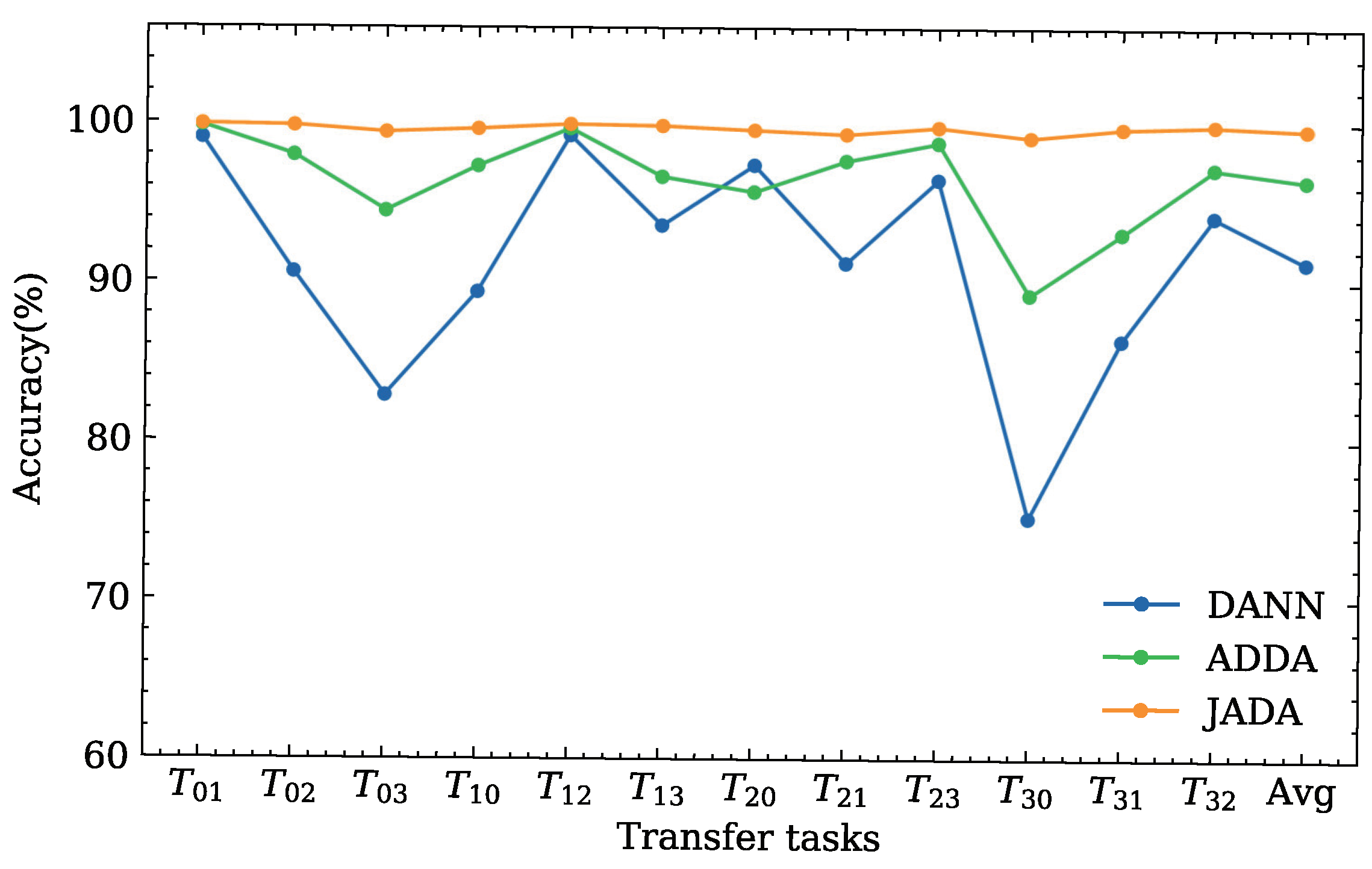
| Transfer Diagnosis Tasks | DANN | ADDA | JADA |
|---|---|---|---|
| 99.03 | 99.81 | 99.87 | |
| 90.61 | 97.95 | 99.80 | |
| 82.86 | 94.46 | 99.40 | |
| 89.37 | 97.29 | 99.62 | |
| 99.22 | 99.66 | 99.92 | |
| 93.58 | 96.65 | 99.84 | |
| 97.39 | 95.71 | 99.59 | |
| 91.24 | 97.68 | 99.35 | |
| 96.49 | 98.81 | 99.80 | |
| 75.23 | 89.27 | 99.16 | |
| 86.41 | 93.13 | 99.73 | |
| 94.18 | 97.21 | 99.91 | |
| Avg | 91.30 | 96.46 | 99.67 |
Publisher’s Note: MDPI stays neutral with regard to jurisdictional claims in published maps and institutional affiliations. |
© 2022 by the authors. Licensee MDPI, Basel, Switzerland. This article is an open access article distributed under the terms and conditions of the Creative Commons Attribution (CC BY) license (https://creativecommons.org/licenses/by/4.0/).
Share and Cite
Zhao, X.; Shao, F.; Zhang, Y. A Novel Joint Adversarial Domain Adaptation Method for Rotary Machine Fault Diagnosis under Different Working Conditions. Sensors 2022, 22, 9007. https://doi.org/10.3390/s22229007
Zhao X, Shao F, Zhang Y. A Novel Joint Adversarial Domain Adaptation Method for Rotary Machine Fault Diagnosis under Different Working Conditions. Sensors. 2022; 22(22):9007. https://doi.org/10.3390/s22229007
Chicago/Turabian StyleZhao, Xiaoping, Fan Shao, and Yonghong Zhang. 2022. "A Novel Joint Adversarial Domain Adaptation Method for Rotary Machine Fault Diagnosis under Different Working Conditions" Sensors 22, no. 22: 9007. https://doi.org/10.3390/s22229007
APA StyleZhao, X., Shao, F., & Zhang, Y. (2022). A Novel Joint Adversarial Domain Adaptation Method for Rotary Machine Fault Diagnosis under Different Working Conditions. Sensors, 22(22), 9007. https://doi.org/10.3390/s22229007