
Earthquake Event Recognition on Smartphones Based on Neural Network Models


Abstract
:1. Introduction
- Making use of the broad distribution and vast amount of smartphones, we can increase the seismic station density, expand the early warning coverage, and reduce the investment in deploying and operating a traditional EEW system;
- With the Global Navigation Satellite System (GNSS) positioning function embedded in smartphones, the earthquake epicenter can be promptly located;
- APPs are more convenient to develop, update and maintain, and some EEW parameters can be customized according to user needs.
2. Datasets
2.1. Data Sources
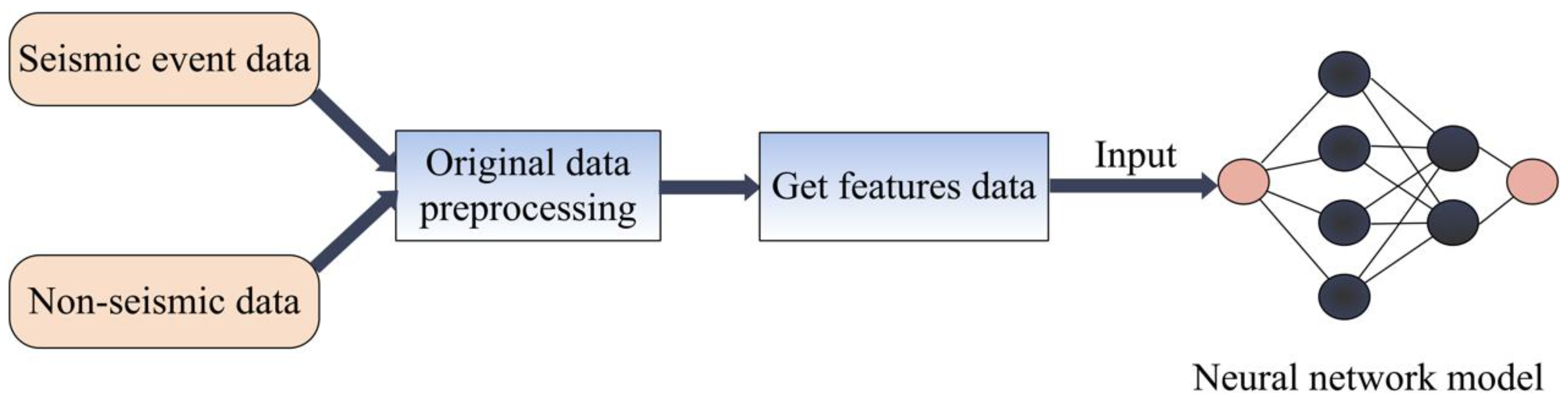
2.2. Data Preprocessing
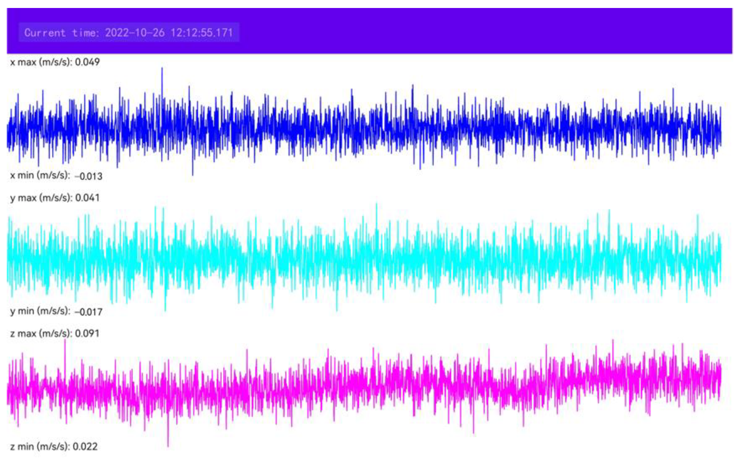
- Removing irrelevant information such as time and location to leave only three-component acceleration;
- Truncating each acceleration record into specified lengths according to different activities (Table 1).
- As to seismic data, the preprocessing steps are:
- Extracting the three-component acceleration data from original files, and merging them into one;
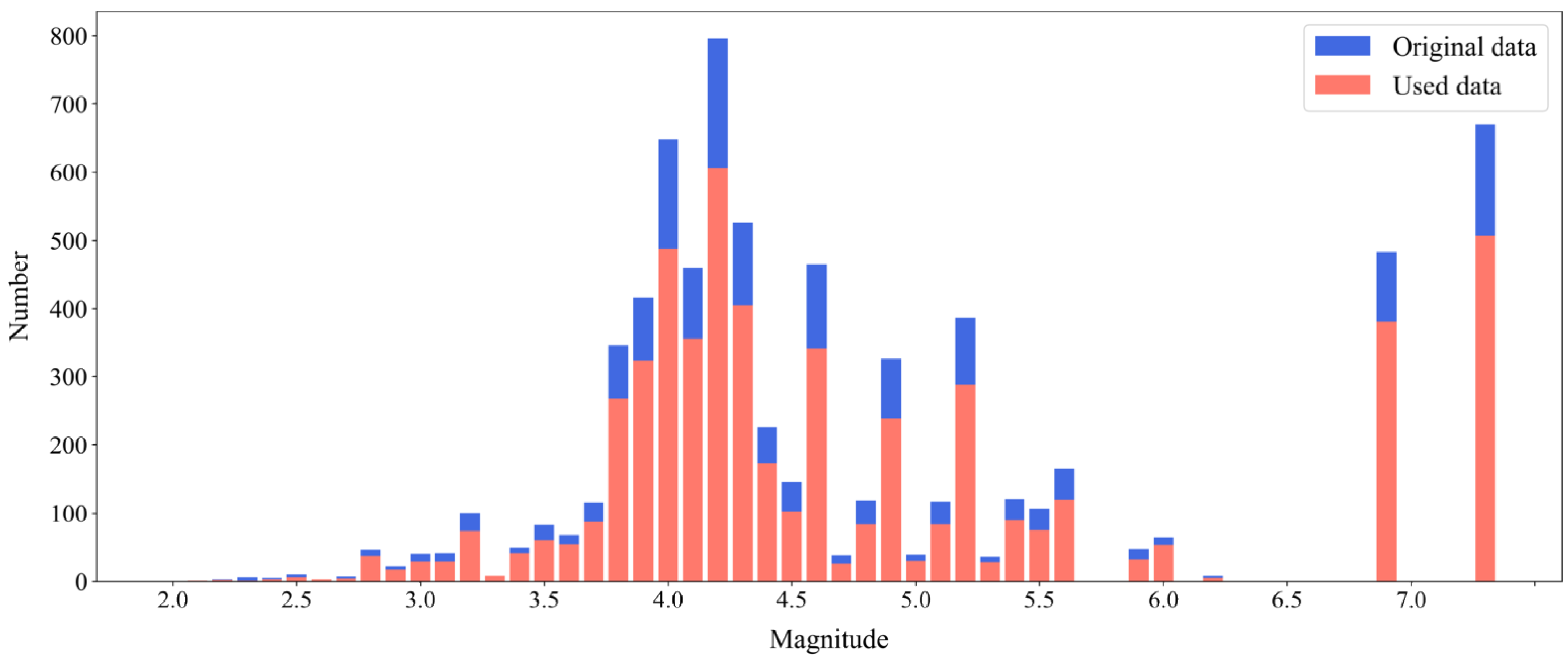
- Manually excluding those data with unclear P wave arrival;
- Detrending each acceleration;
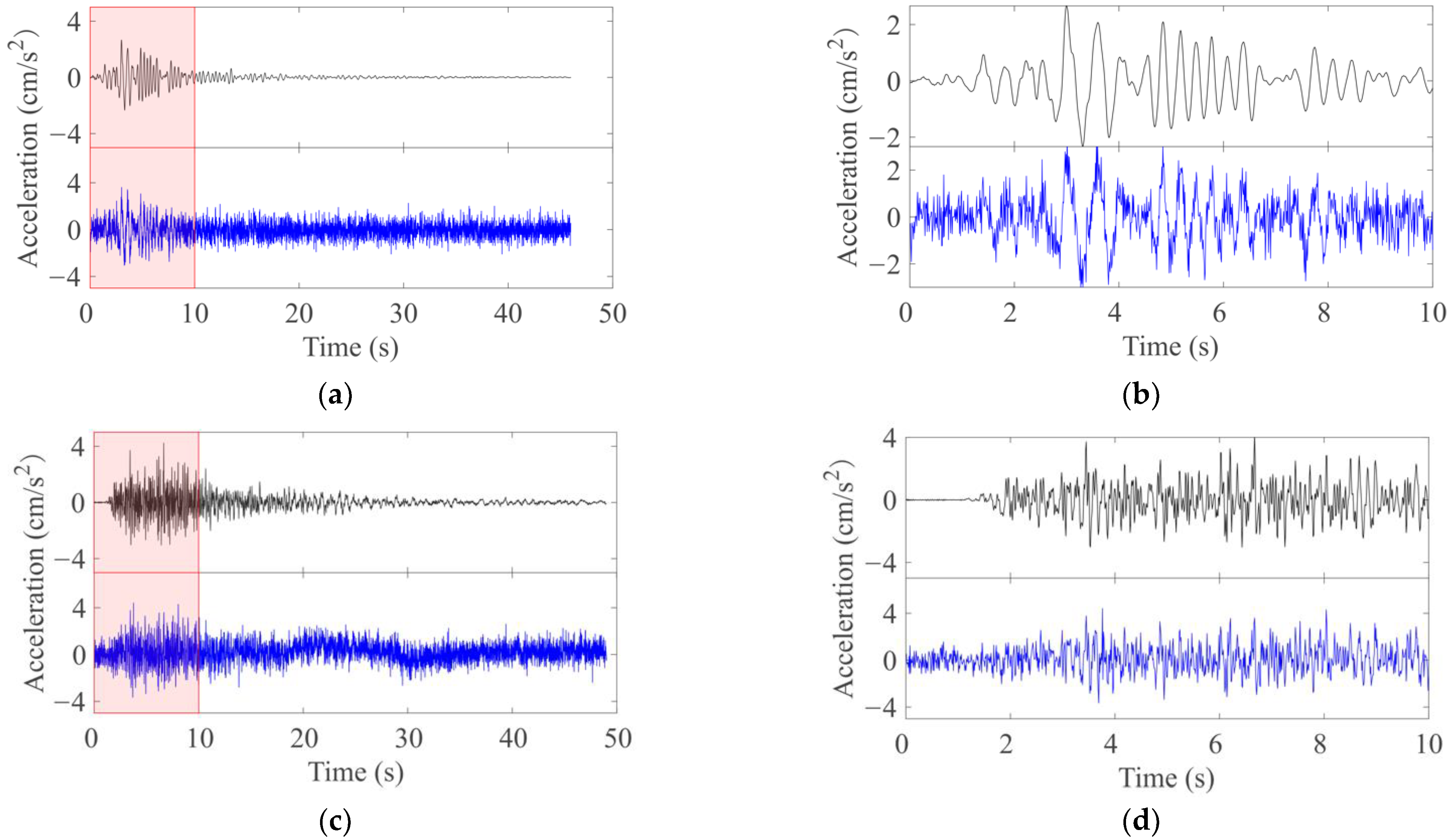
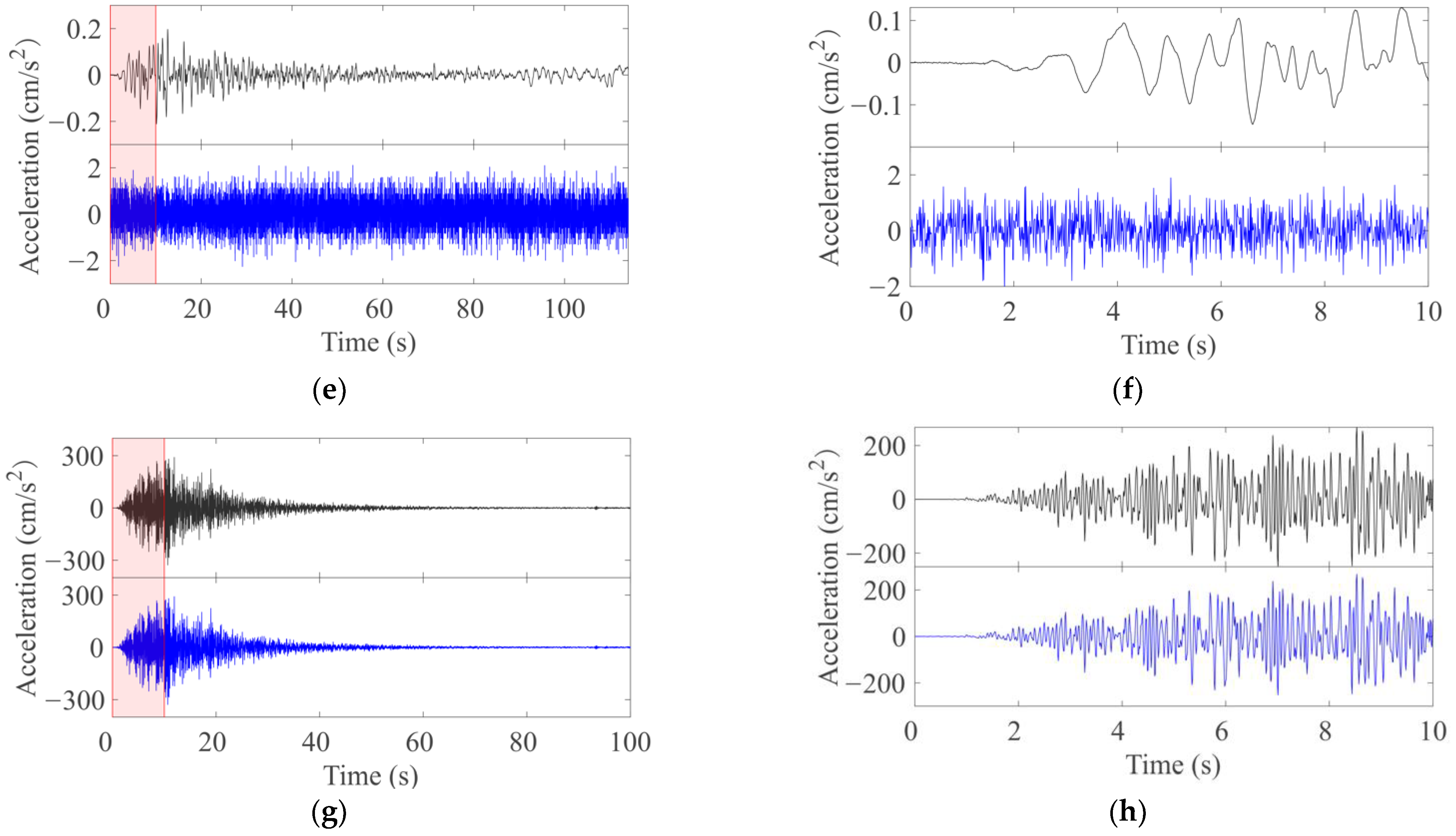
- Adding the mobile phone self-noise to each record for simulating earthquake data recorded by a mobile phone.
3. Methods
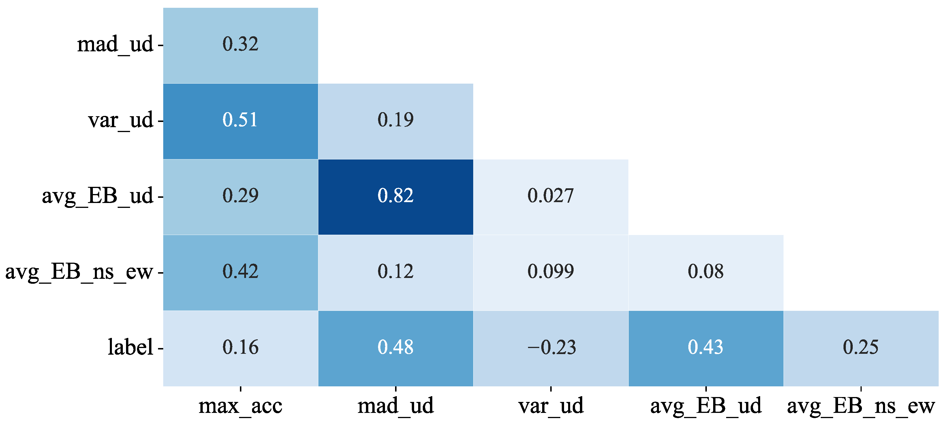
3.1. Feature Selection
| Algorithm 1 PCA code in Python |
| From sklearn.decomposition import PCA |
| estimator = PCA(n_components = 10) # Initialization, n_components is the dimension reduction dimension |
| # Use the training features to determine the orientation of the 10 orthogonal dimensions and transform the original training features |
| pca_X_train = estimator.fit_transform(data_train_x) |
| # The test features are also transformed according to the above-mentioned 10 orthogonal dimension directions (transform) |
| pca_X_test = estimator.transform(data_test_x) |
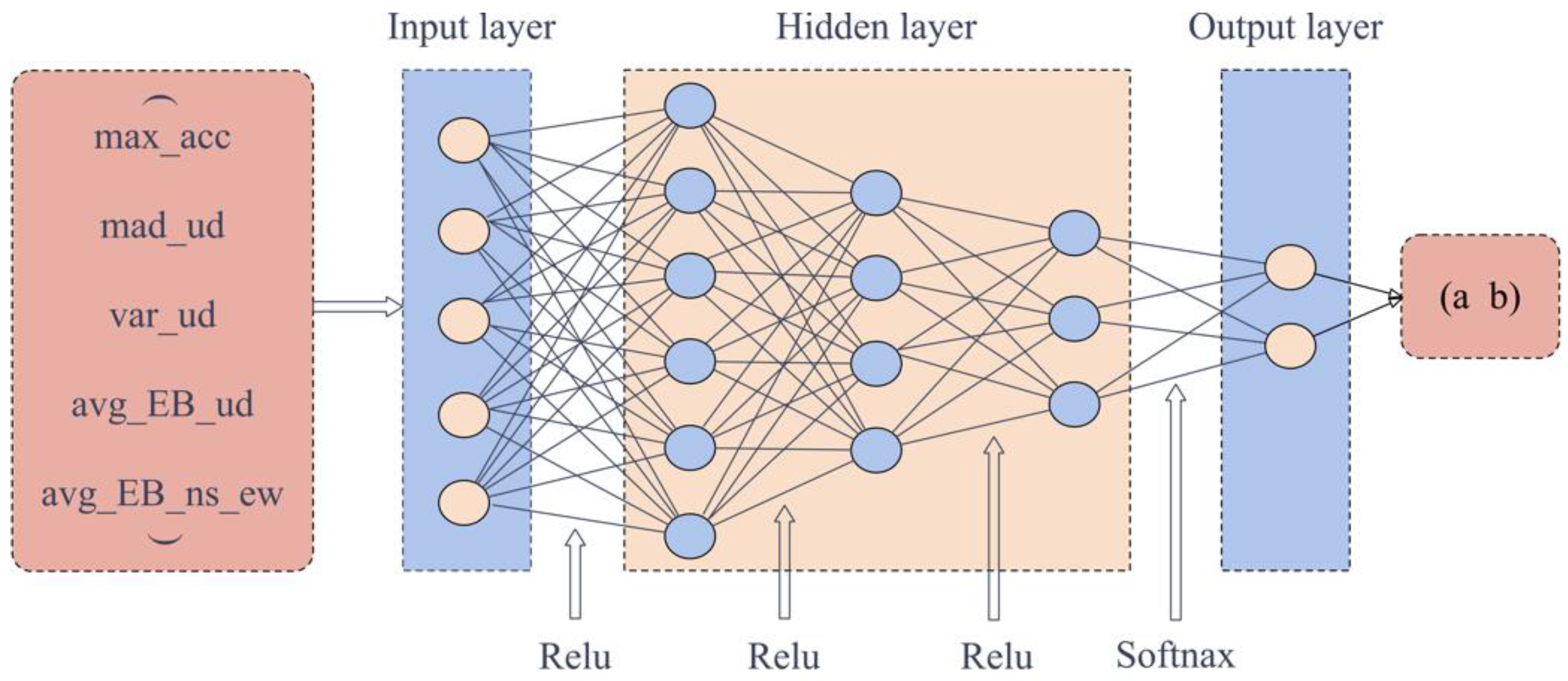
3.2. FCNN
3.2.1. Architecture
3.2.2. Performance
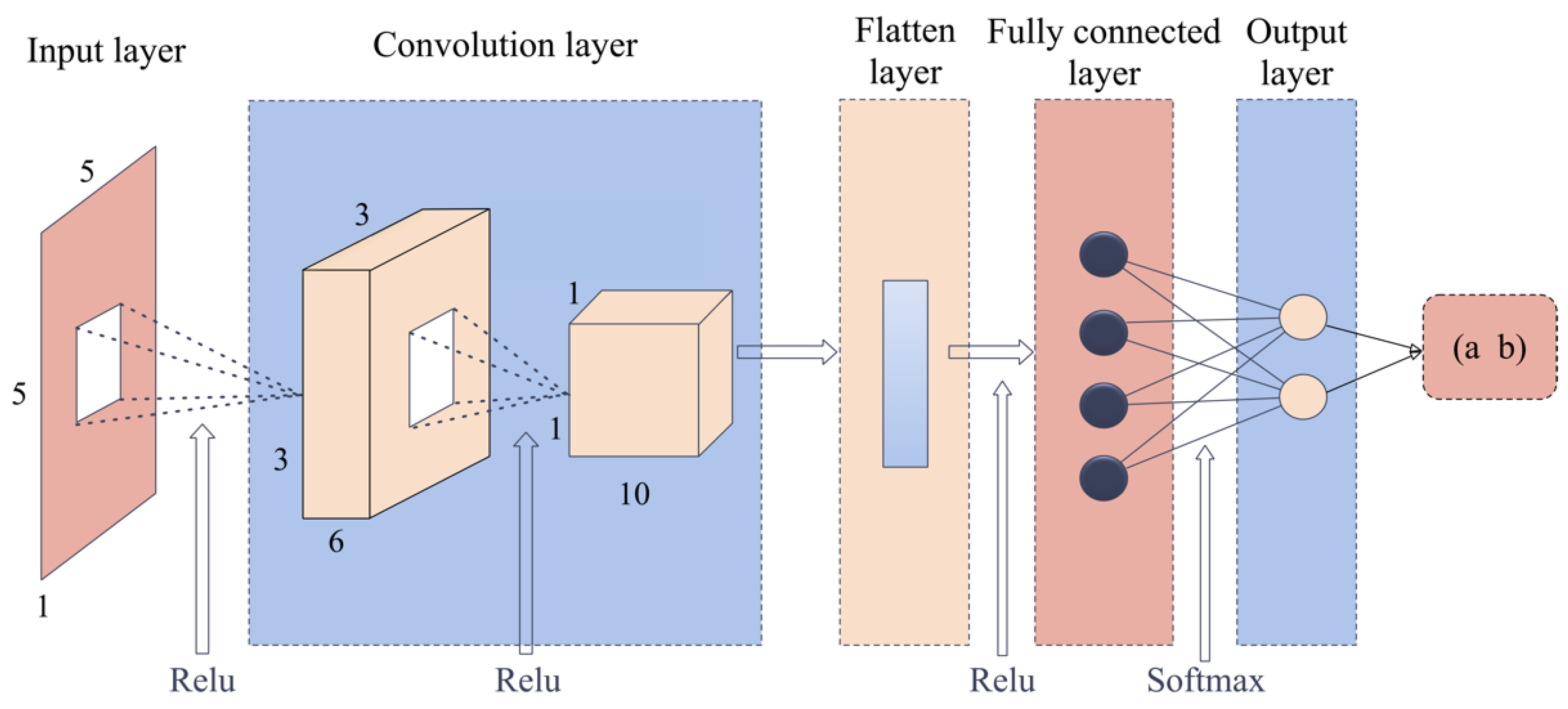
3.3. CNN
3.3.1. Architecture
3.3.2. Performance
3.4. Other Algorithms
4. Discussion
4.1. Comparison of the Results of Different Algorithms
4.2. Can We Apply the Trained Models to an Actual EEW APP?
4.3. Limitations and Corresponding Solutions of EEW on Mobile Phones
- The sensors in mobile phones are not dedicated to detecting earthquakes, so they cannot reach the accuracy of professional strong-motion accelerometers;
- The installed capacity of mobile APPs is determined by the results of user experience, such as power consumption, CPU load, and local storage space occupied. If the installed capacity is insufficient, we will not be able to achieve the goal of trading quantity for quality, making it difficult to carry out EEW.
5. Conclusions
Author Contributions
Funding
Institutional Review Board Statement
Informed Consent Statement
Data Availability Statement
Acknowledgments
Conflicts of Interest
References
- Peng, C.; Jiang, P.; Ma, Q.; Su, J.; Cai, Y.; Zheng, Y. Chinese Nationwide Earthquake Early Warning System and Its Performance in the 2022 Lushan M 6.1 Earthquake. Remote Sens. 2022, 14, 4269. [Google Scholar] [CrossRef]
- Wu, Y.M.; Mittal, H.; Chen, D.Y.; Hsu, T.Y.; Lin, P.Y. Earthquake early warning systems in Taiwan: Current status. J. Geol. Soc. India 2022, 97, 1525–1532. [Google Scholar] [CrossRef]
- Kohler, M.D.; Cochran, E.S.; Given, D.; Guiwits, S.; Neuhauser, D.; Henson, I.; Hartog, R.; Bodin, P.; Kress, V.; Thompson, S.; et al. Earthquake early warning ShakeAlert system: West coast wide production prototype. Seismol. Res. Lett. 2018, 89, 99–107. [Google Scholar] [CrossRef] [Green Version]
- Festa, G.; Picozzi, M.; Caruso, A.; Colombelli, S.; Cattaneo, M.; Chiaraluce, L.; Elia, L.; Martino, C.; Marzorati, S.; Supino, M.; et al. Performance of earthquake early warning systems during the 2016–2017 Mw 5–6.5 Central Italy sequence. Seismol. Res. Lett. 2018, 89, 1–12. [Google Scholar] [CrossRef]
- Cuéllar, A.; Suárez, G.; Espinosa-Aranda, J.M. Performance evaluation of the earthquake detection and classification algorithm 2 (t S–t P) of the Seismic Alert System of Mexico (SASMEX). Bull. Seismol. Soc. Am. 2017, 107, 1451–1463. [Google Scholar] [CrossRef]
- Kodera, Y.; Hayashimoto, N.; Tamaribuchi, K.; Noguchi, K.; Moriwaki, K.; Takahashi, R.; Morimoto, M.; Okamoto, K.; Hoshiba, M. Developments of the Nationwide Earthquake Early Warning System in Japan After the 2011 M w 9.0 Tohoku-Oki Earthquake. Front. Earth Sci. 2021, 9, 726045. [Google Scholar] [CrossRef]
- Wu, Y.M.; Chen, D.Y.; Lin, T.L.; Hsieh, C.Y.; Chin, T.L.; Chang, W.Y.; Li, W.S.; Ker, S.H. A High-Density Seismic Network for Earthquake Early Warning in Taiwan Based on Low Cost Sensors. Seismol. Res. Lett. 2013, 84, 1049. [Google Scholar] [CrossRef]
- Wu, Y.M.; Liang, W.T.; Mittal, H.; Chao, W.A.; Lin, C.H.; Huang, B.S.; Lin, C.M. Performance of a low-cost earthquake early warning system (P-alert) during the 2016 ML 6.4 Meinong (Taiwan) earthquake. Seismol. Res. Lett. 2016, 87, 1050–1059. [Google Scholar] [CrossRef]
- Evans, J.R.; Allen, R.M.; Chung, A.I.; Cochran, E.S.; Guy, R.; Hellweg, M.; Lawrence, J.F. Performance of several low-cost accelerometers. Seismol. Res. Lett. 2014, 85, 147–158. [Google Scholar] [CrossRef]
- Wu, Y.M.; Lin, T.L. A test of earthquake early warning system using low cost accelerometer in Hualien, Taiwan. In Early Warning for Geological Disasters; Springer: Berlin/Heidelberg, Germany, 2014; pp. 253–261. [Google Scholar] [CrossRef]
- Peng, C.; Jiang, P.; Chen, Q.; Ma, Q.; Yang, J. Performance evaluation of a dense MEMS-based seismic sensor array deployed in the Sichuan-Yunnan border region for earthquake early warning. Micromachines 2019, 10, 735. [Google Scholar] [CrossRef] [Green Version]
- Wu, Y.M.; Mittal, H. A review on the development of earthquake warning system using low-cost sensors in Taiwan. Sensors 2021, 21, 7649. [Google Scholar] [CrossRef]
- Dashti, S.; Bray, J.D.; Reilly, J.; Glaser, S.; Bayen, A.; Mari, E. Evaluating the reliability of phones as seismic monitoring instruments. Earthq. Spectra 2014, 30, 721–742. [Google Scholar] [CrossRef] [Green Version]
- Uga, T.; Nagaosa, T.; Kawashima, D. An emergency earthquake warning system using mobile terminals with a built-in accelerometer. In Proceedings of the 2012 IEEE 12th International Conference on ITS Telecommunications, Taipei, Taiwan, 5–8 November 2012; pp. 837–842. [Google Scholar] [CrossRef]
- Naito, S.; Azuma, H.; Senna, S.; Yoshizawa, M.; Nakamura, H.; Hao, K.X.; Fujiwara, H.; Hirayama, Y.; Yuki, N.; Yoshida, M. Development and testing of a mobile application for recording and analyzing seismic data. J. Disaster Res. 2013, 8, 990–1000. [Google Scholar] [CrossRef]
- Reilly, J.; Dashti, S.; Ervasti, M.; Bray, J.D.; Glaser, S.D.; Bayen, A.M. Mobile phones as seismologic sensors: Automating data extraction for the iShake system. IEEE Trans. Autom. Sci. Eng. 2013, 10, 242–251. [Google Scholar] [CrossRef]
- Kong, Q.; Allen, R.M.; Schreier, L.; Kwon, Y.W. MyShake—A smartphone app to detect earthquakes. In Proceedings of the AGU Fall Meeting Abstract, San Francisco, CA, USA, 14–18 December 2015; p. T13D-3032. [Google Scholar]
- Finazzi, F. The earthquake network project: Toward a crowdsourced smartphone-based earthquake early warning system. Bull. Seismol. Soc. Am. 2016, 106, 1088–1099. [Google Scholar] [CrossRef] [Green Version]
- Zambrano, O.M.; Zambrano, A.M.; Esteve, M.; Palau, C. An Innovative and Economic Management of Earthquakes: Early Warnings and Situational Awareness in Real Time. In Wireless Public Safety Networks 3; Elsevier Ltd.: Amsterdam, The Netherlands, 2017; pp. 19–38. [Google Scholar] [CrossRef]
- Bossu, R.; Steed, R.; Roussel, F.; Landès, M.; Fuenzalida, A.; Matrullo, E.; Dupont, A.; Roch, J.; Fallou, L. App earthquake detection and automatic mapping of felt area. Seismol. Res. Lett. 2019, 90, 305–312. [Google Scholar] [CrossRef]
- Colombelli, S.; Carotenuto, F.; Elia, L.; Zollo, A. Design and implementation of a mobile device app for network-based earthquake early warning systems (EEWSs): Application to the PRESTo EEWS in southern Italy. Nat. Hazards Earth Syst. Sci. 2020, 20, 921–931. [Google Scholar] [CrossRef]
- Hsu, T.Y.; Nieh, C.P. On-site earthquake early warning using smartphones. Sensors 2020, 20, 2928. [Google Scholar] [CrossRef] [PubMed]
- Kong, Q.; Allen, R.M.; Schreier, L.; Kwon, Y.W. MyShake: A smartphone seismic network for earthquake early warning and beyond. Sci. Adv. 2016, 2, e1501055. [Google Scholar] [CrossRef] [PubMed] [Green Version]
- Kong, Q.; Allen, R.M.; Allen, S.; Bair, T.; Meja, A.; Patel, S.; Strauss, J.; Thompson, S. Crowdsourcing Felt Reports using the MyShake smartphone app. arXiv 2022, arXiv:2204.12675. [Google Scholar] [CrossRef]
- Allen, R.M.; Kong, Q.; Martin-Short, R. The myshake platform: A global vision for earthquake early warning. Pure Appl. Geophys. 2020, 177, 1699–1712. [Google Scholar] [CrossRef] [Green Version]
- Bossu, R.; Finazzi, F.; Steed, R.; Fallou, L.; Bondár, I. “Shaking in 5 seconds!” A Voluntary Smartphone-based Earthquake Early Warning System. arXiv 2021, arXiv:2102.06739. [Google Scholar] [CrossRef]
- Kumar, S.; Vig, R.; Kapur, P. Development of earthquake event detection technique based on STA/LTA algorithm for seismic alert system. J. Geol. Soc. India 2018, 92, 679–686. [Google Scholar] [CrossRef]
- Zhang, J.; Tang, Y.; Li, H. STA/LTA Fractal Dimension Algorithm of Detecting the P-Wave Arrival. Bull. Seismol. Soc. Am. 2014, 108, 230–237. [Google Scholar] [CrossRef]
- Giridhar, U.S.; Prajapati, N.; Sonkusare, R. Analysis and Determination of Magnitude of Earthquake Using STA-LTA Algorithm. In Proceedings of the 2021 12th International Conference on Computing Communication and Networking Technologies (ICCCNT), Kharagpur, India, 6–8 July 2021; pp. 1–5. [Google Scholar] [CrossRef]
- Khalqillah, A.; Isa, M.; Muksin, U. A GUI based automatic detection of seismic P-wave arrivals by using Short Term Average/Long Term Average (STA/LTA) method. In Journal of Physics: Conference Series; IOP Publishing Ltd.: Bristol, UK, 2018; p. 032014. [Google Scholar] [CrossRef]
- Choubik, Y.; Mahmoudi, A.; Himmi, M.M.; El Moudnib, L. STA/LTA trigger algorithm implementation on a seismological dataset using Hadoop MapReduce. IAES Int. J. Artif. Intell. 2020, 9, 269. [Google Scholar] [CrossRef]
- Akaike, H. A new look at the statistical model identification. IEEE Trans. Automat. Contr. 1974, 19, 716–723. [Google Scholar] [CrossRef]
- Zhang, H.; Thurber, C.; Rowe, C. Automatic P-wave arrival detection and picking with multiscale wavelet analysis for single-component recordings. Bull. Seismol. Soc. Am. 2003, 93, 1904–1912. [Google Scholar] [CrossRef] [Green Version]
- Shen, T.; Tuo, X.; Li, H.; Liu, Y.; Rong, W. A first arrival picking method of microseismic data based on single time window with window length independent. J. Seismol. 2018, 22, 1613–1627. [Google Scholar] [CrossRef]
- Zhu, M.; Wang, L.; Liu, X.; Zhao, J. Accurate identification of microseismic P-and S-phase arrivals using the multi-step AIC algorithm. J. Appl. Geophys. 2018, 150, 284–293. [Google Scholar] [CrossRef]
- Shang, X.; Li, X.; Morales-Esteban, A.; Dong, L. Enhancing micro-seismic P-phase arrival picking: EMD-cosine function-based denoising with an application to the AIC picker. J. Appl. Geophys. 2018, 150, 325–337. [Google Scholar] [CrossRef]
- Long, Y.; Lin, J.; Li, B.; Wang, H.; Chen, Z. Fast-AIC method for automatic first arrivals picking of microseismic event with multitrace energy stacking envelope summation. IEEE Geosci. Remote Sens. Lett. 2019, 17, 1832–1836. [Google Scholar] [CrossRef]
- Nakamula, S.; Takeo, M.; Okabe, Y.; Matsuura, M. Automatic seismic wave arrival detection and picking with stationary analysis: Application of the KM2O-Langevin equations. Earth Planets Space 2007, 59, 567–577. [Google Scholar] [CrossRef] [Green Version]
- Zhang, H.; Melgar, D.; Sahakian, V.; Searcy, J.; Lin, J.T. Learning source, path and site effects: CNN-based on-site intensity prediction for earthquake early warning. Geophys. J. Int. 2022, 231, 2186–2204. [Google Scholar] [CrossRef]
- Bilal, M.A.; Ji, Y.; Wang, Y.; Akhter, M.P.; Yaqub, M. Early Earthquake Detection Using Batch Normalization Graph Convolutional Neural Network (BNGCNN). Appl. Sci. 2022, 12, 7548. [Google Scholar] [CrossRef]
- van den Ende, M.P.; Ampuero, J.P. Automated seismic source characterization using deep graph neural networks. Geophys. Res. Lett. 2020, 47, e2020GL088690. [Google Scholar] [CrossRef]
- Wang, C.Y.; Huang, T.C.; Wu, Y.M. Using LSTM Neural Networks for Onsite Earthquake Early Warning. Seismol. Res. Lett. 2022, 93, 814–826. [Google Scholar] [CrossRef]
- Abdalzaher, M.S.; Soliman, M.S.; El-Hady, S.M.; Benslimane, A.; Elwekeil, M. A deep learning model for earthquake parameters observation in IoT system-based earthquake early warning. IEEE Internet Things J. 2021, 9, 8412–8424. [Google Scholar] [CrossRef]
- Zhu, J.; Li, S.; Song, J.; Wang, Y. Magnitude estimation for earthquake early warning using a deep convolutional neural network. Front. Earth Sci. 2021, 341. [Google Scholar] [CrossRef]
- Perol, T.; Gharbi, M.; Denolle, M. Convolutional neural network for earthquake detection and location. Sci. Adv. 2018, 4, e1700578. [Google Scholar] [CrossRef] [Green Version]
- Li, X. Seismic Event Detection Based on Smartphone Accelerometer. Master’s Thesis, Wuhan University, Wuhan, China, 2017. (in Chinese with English abstract). Available online: https://kns.cnki.net/KCMS/detail/detail.aspx?dbname=CMFD201802&filename=1017179688.nh (accessed on 1 November 2022).
- Feldbusch, A.; Sadegh-Azar, H.; Agne, P. Vibration analysis using mobile devices (smartphones or tablets). Procedia Eng. 2017, 199, 2790–2795. [Google Scholar] [CrossRef]
- Mariani, M.C.; Tweneboah, O.K.; Beccar-Varela, M.P. Principal Component Analysis. In Data Science in Theory and Practice: Techniques for Big Data Analytics and Complex Data Sets; John Wiley & Sons: New York, NY, USA, 2021; pp. 151–163. [Google Scholar] [CrossRef]
- Towards Data Science. Available online: https://towardsdatascience.com/under-the-hood-of-neural-networks-part-1-fully-connected-5223b7f78528 (accessed on 13 October 2022).
- Pal, K.K.; Sudeep, K.S. Preprocessing for image classification by convolutional neural networks. In Proceedings of the 2016 IEEE International Conference on Recent Trends in Electronics, Information & Communication Technology (RTEICT), Bangalore, India, 20–21 May 2016; pp. 1778–1781. [Google Scholar] [CrossRef]
- Francis, M.; Deisy, C. Disease detection and classification in agricultural plants using convolutional neural networks—A visual understanding. In Proceedings of the 2019 6th International Conference on Signal Processing and Integrated Networks (SPIN), Noida, India, 7–8 March 2019; pp. 1063–1068. [Google Scholar] [CrossRef]
- Ruderman, A.; Rabinowitz, N.C.; Morcos, A.S.; Zoran, D. Pooling is neither necessary nor sufficient for appropriate deformation stability in CNNs. arXiv 2018, arXiv:1804.04438. [Google Scholar] [CrossRef]
- Zheng, Z.; Wang, J.; Shi, L.; Zhao, S.; Hou, J.; Sun, L.; Dong, L. Generating phone-quality records to train machine learning models for smartphone-based earthquake early warning. J. Seismol. 2022, 26, 439–454. [Google Scholar] [CrossRef]
- Inbal, A.; Kong, Q.; Savran, W.; Allen, R.M. On the feasibility of using the dense MyShake smartphone array for earthquake location. Seismol. Res. Lett. 2019, 90, 1209–1218. [Google Scholar] [CrossRef] [Green Version]
- Inbal, A.; Ampuero, J.P.; Clayton, R.W. Localized seismic deformation in the upper mantle revealed by dense seismic arrays. Science 2016, 354, 88–92. [Google Scholar] [CrossRef] [Green Version]
- Inbal, A.; Clayton, R.W.; Ampuero, J.P. Imaging widespread seismicity at midlower crustal depths beneath Long Beach, CA, with a dense seismic array: Evidence for a depth-dependent earthquake size distribution. Geophys. Res. Lett. 2015, 42, 6314–6323. [Google Scholar] [CrossRef] [Green Version]
- da Silva, S.L.E.; Corso, G. Microseismic event detection in noisy environments with instantaneous spectral Shannon entropy. Phys. Rev. E 2022, 106, 014133. [Google Scholar] [CrossRef]


| Phone Model | Data Type | Phone’s Location | Velocity | Data Length (Second) |
|---|---|---|---|---|
| Vivo S5 Huawei nova 5pro Xiaomi 8se | Walking | In hands/In bags | Low/Normal/Fast | 90 |
| Running | In hands/In bags | Low/Fast | ||
| Going up and down stairs | In hands/In bags | Normal | ||
| Riding a bike | In bags | |||
| Taking the bus | In hands/In bags | 30/35/60/90 | ||
| Taking the subway | In hands/In bags |
| Feature Name | Number of Features | Calculation Formula | Explanation |
|---|---|---|---|
| The peak acceleration in a frame | 1 | ) | x, y, z: EW, NS, UD at a certain moment i: index, the value is [1, N] : the third and the first quartile S: a component data, such as EW, NS, or UD N: data length average of UD |
| The average acceleration in a frame | 1 | ||
| The absolute median deviation | 3 | ||
| Interquartile range (IQR) | 3 | ||
| Variance | 3 | ||
| Standard deviation | 3 | ||
| Average time-domain energy | 3 | ||
| Horizontal average time-domain energy | 1 |
| Feature Dimension | Average Validation Accuracy | Best Test Accuracy |
|---|---|---|
| 10 | 78.98% | 97.33% |
| 8 | 78.92% | 99.25% |
| 5 | 78.7% | 99.04% |
| 3 | 77.39% | 99.22% |
| Hidden Layers | Number of Nodes | Average Validation Accuracy | Best Test Accuracy | Training Time (Second) |
|---|---|---|---|---|
| 2 | 4, 3 | 98.77% | 98.4% | 150 |
| 3 | 6, 4, 3 | 99.06% | 98.83% | 196 |
| 4 | 8, 6, 4, 3 | 99.23% | 99.46% | 246 |
| 5 | 10, 8, 6, 4, 3 | 99.27% | 99.36% | 291 |
| 6 | 12, 10, 8, 6, 4, 3 | 99.29% | 99.37% | 360 |
Publisher’s Note: MDPI stays neutral with regard to jurisdictional claims in published maps and institutional affiliations. |
© 2022 by the authors. Licensee MDPI, Basel, Switzerland. This article is an open access article distributed under the terms and conditions of the Creative Commons Attribution (CC BY) license (https://creativecommons.org/licenses/by/4.0/).
Share and Cite
Chen, M.; Peng, C.; Cheng, Z. Earthquake Event Recognition on Smartphones Based on Neural Network Models. Sensors 2022, 22, 8769. https://doi.org/10.3390/s22228769
Chen M, Peng C, Cheng Z. Earthquake Event Recognition on Smartphones Based on Neural Network Models. Sensors. 2022; 22(22):8769. https://doi.org/10.3390/s22228769
Chicago/Turabian StyleChen, Meirong, Chaoyong Peng, and Zhenpeng Cheng. 2022. "Earthquake Event Recognition on Smartphones Based on Neural Network Models" Sensors 22, no. 22: 8769. https://doi.org/10.3390/s22228769
APA StyleChen, M., Peng, C., & Cheng, Z. (2022). Earthquake Event Recognition on Smartphones Based on Neural Network Models. Sensors, 22(22), 8769. https://doi.org/10.3390/s22228769