
Physics-Informed Data-Driven Prediction of 2D Normal Strain Field in Concrete Structures


Abstract
1. Introduction
2. Materials and Methods
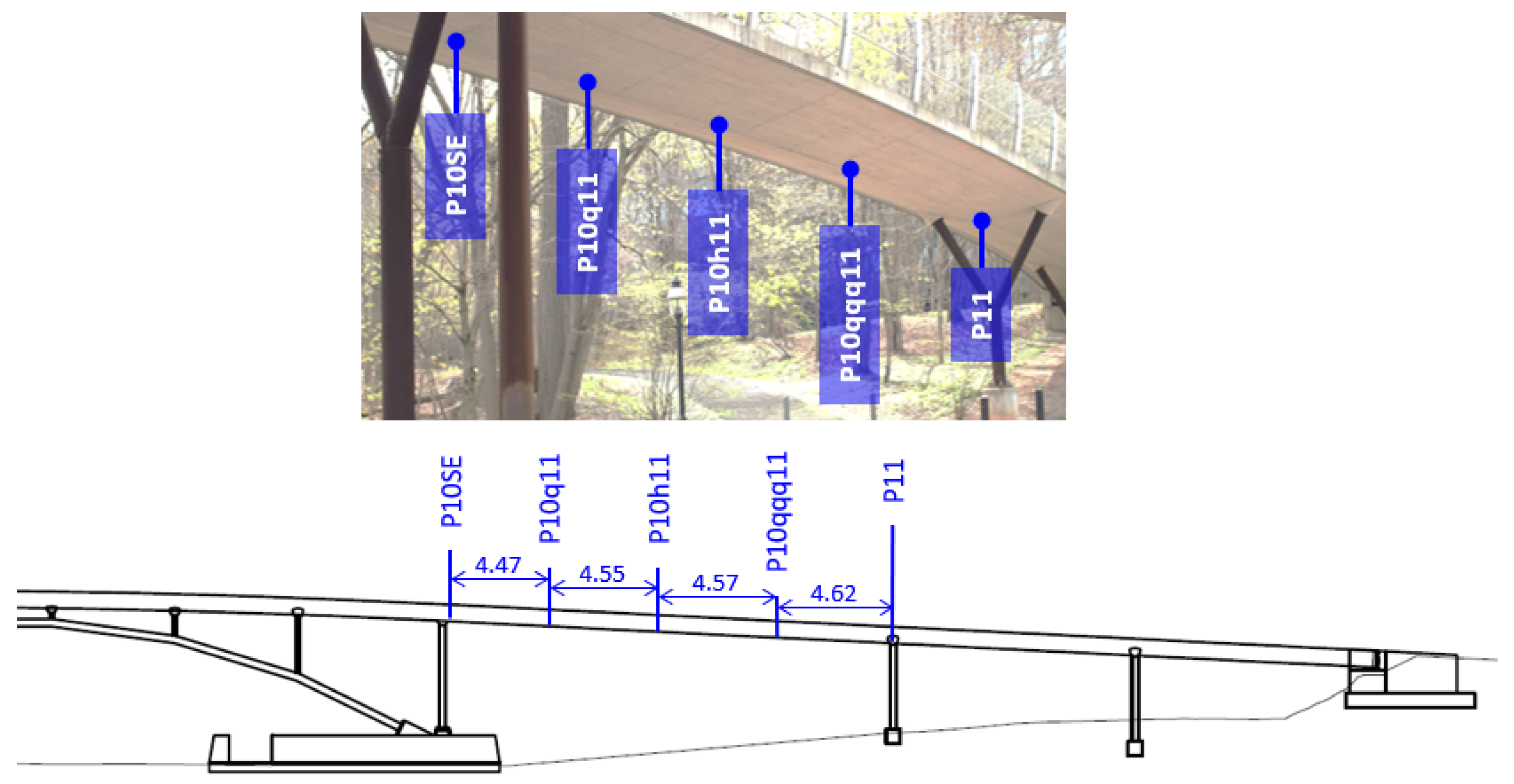
2.1. Streicker Bridge
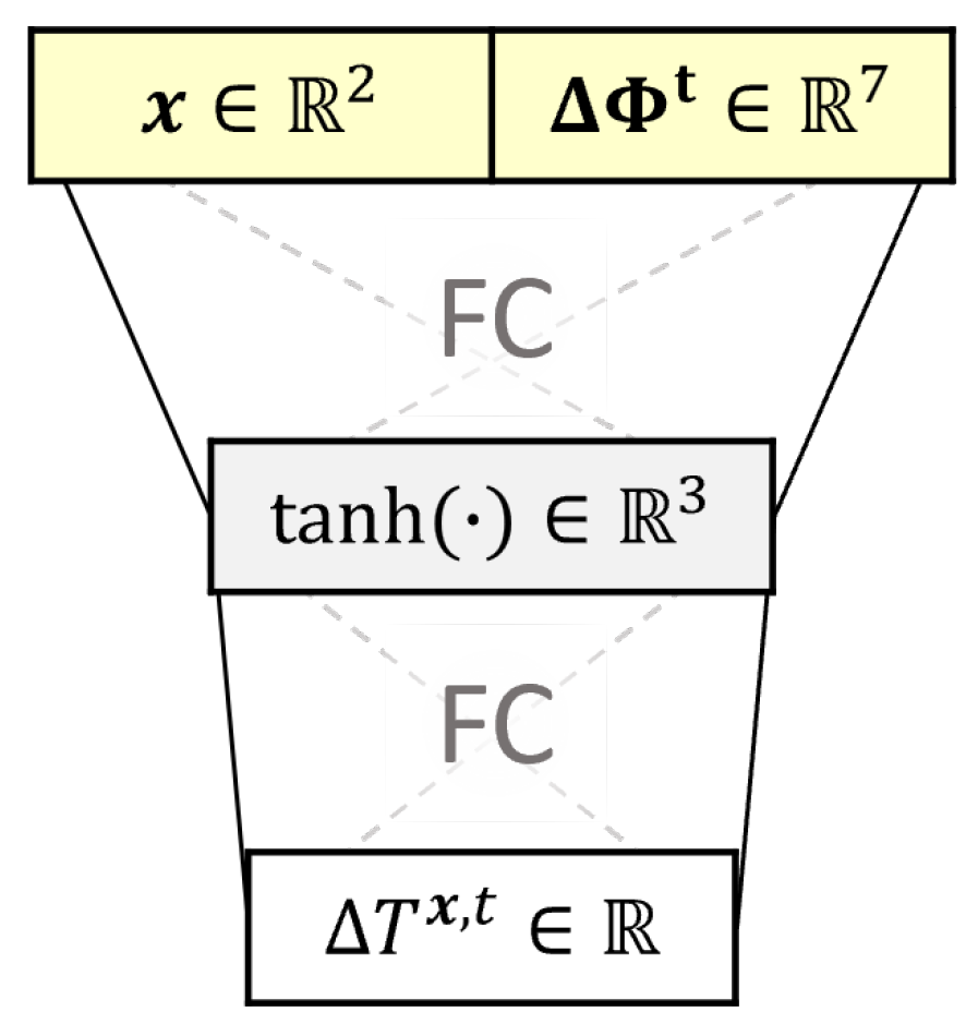
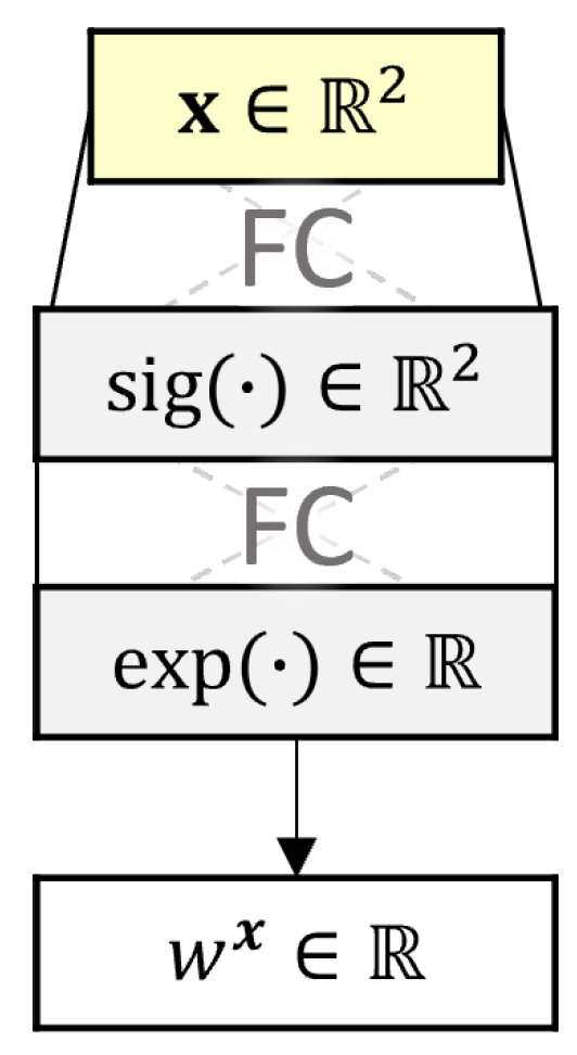
2.2. Total Strain Change Model
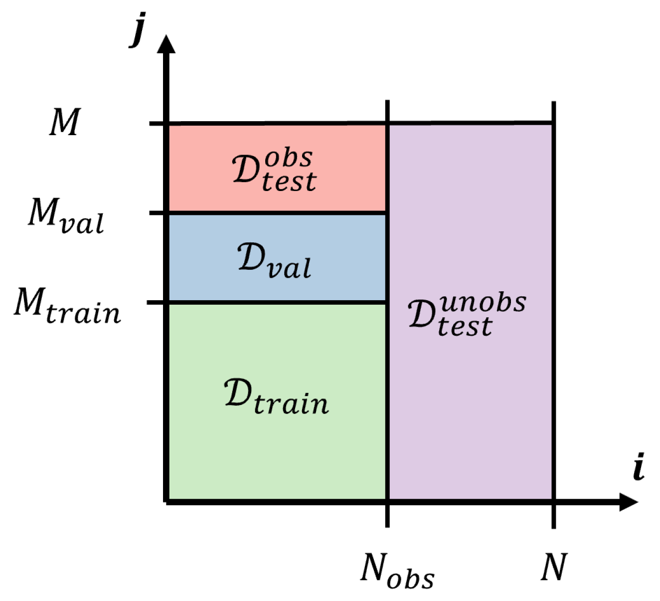
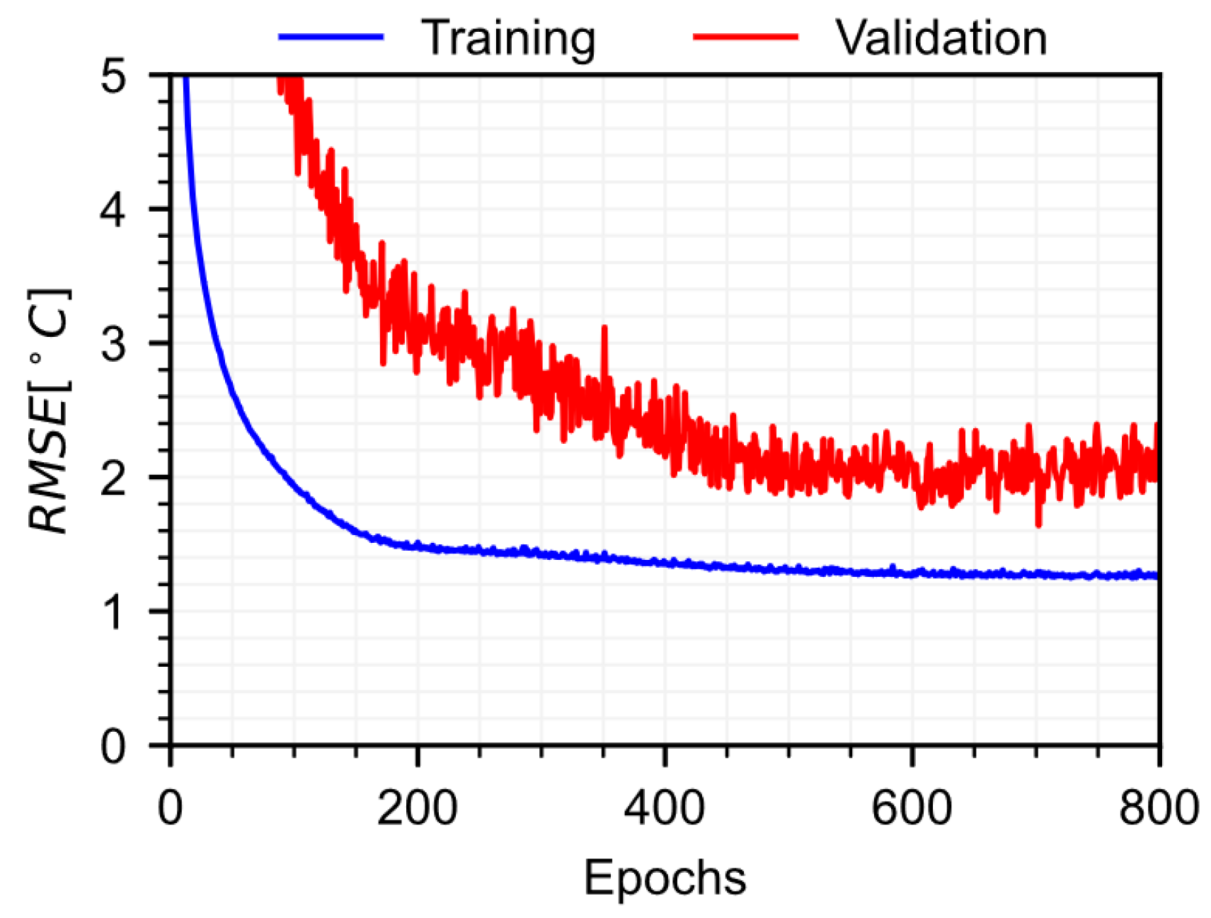
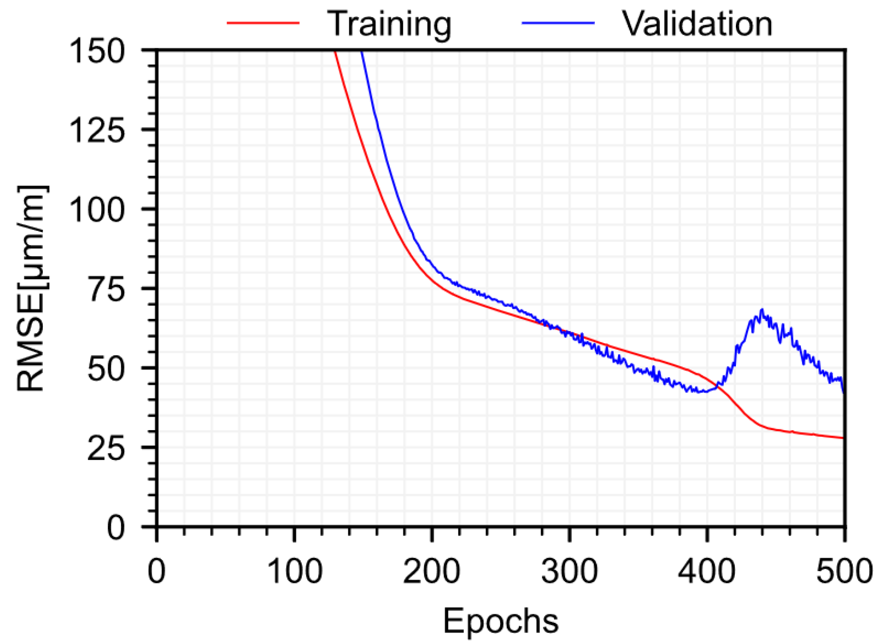
2.3. Model Training
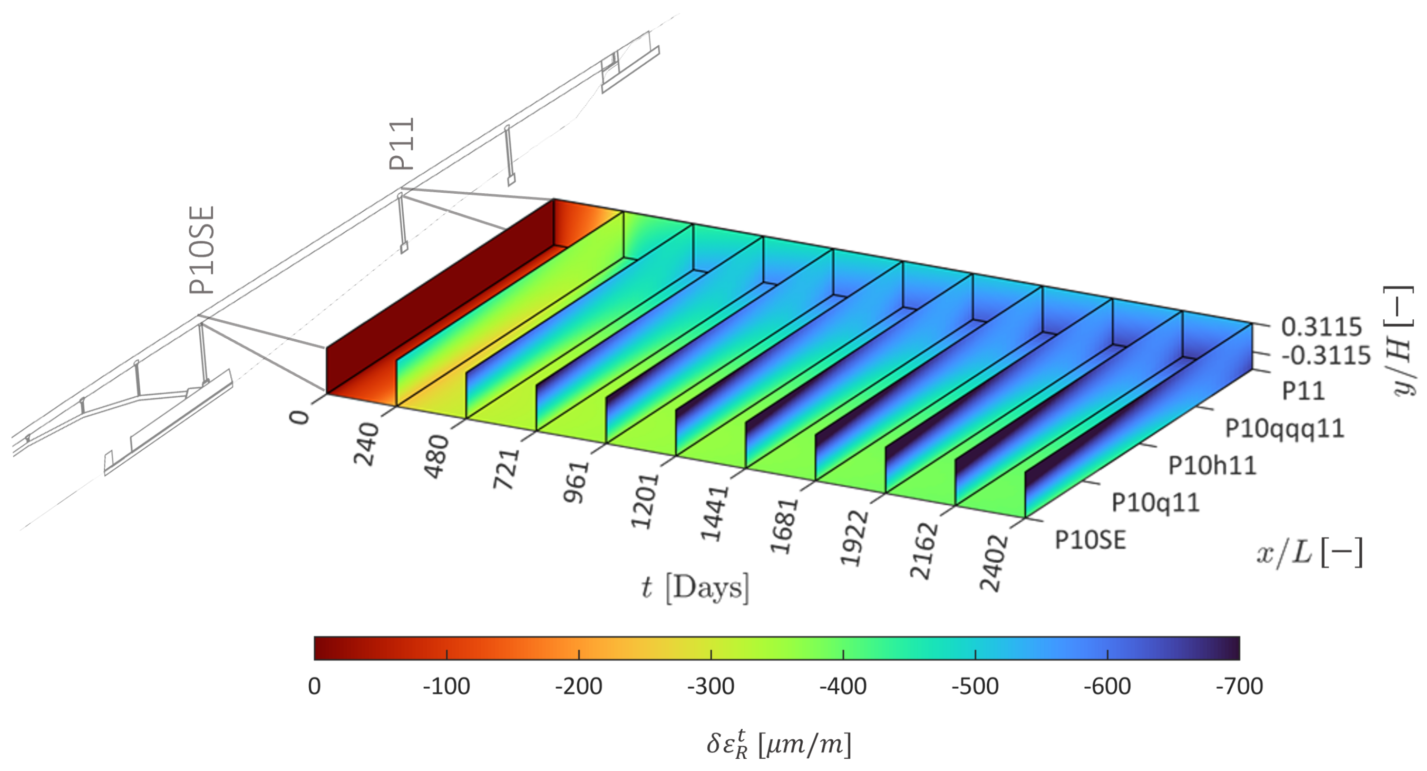
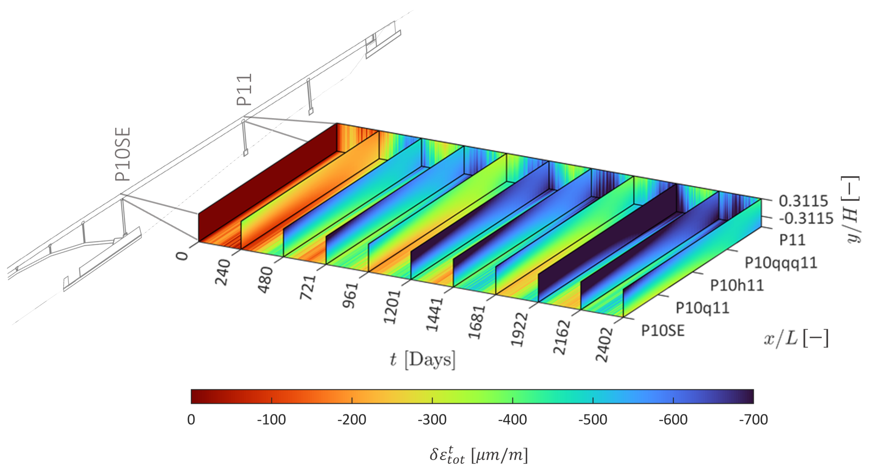
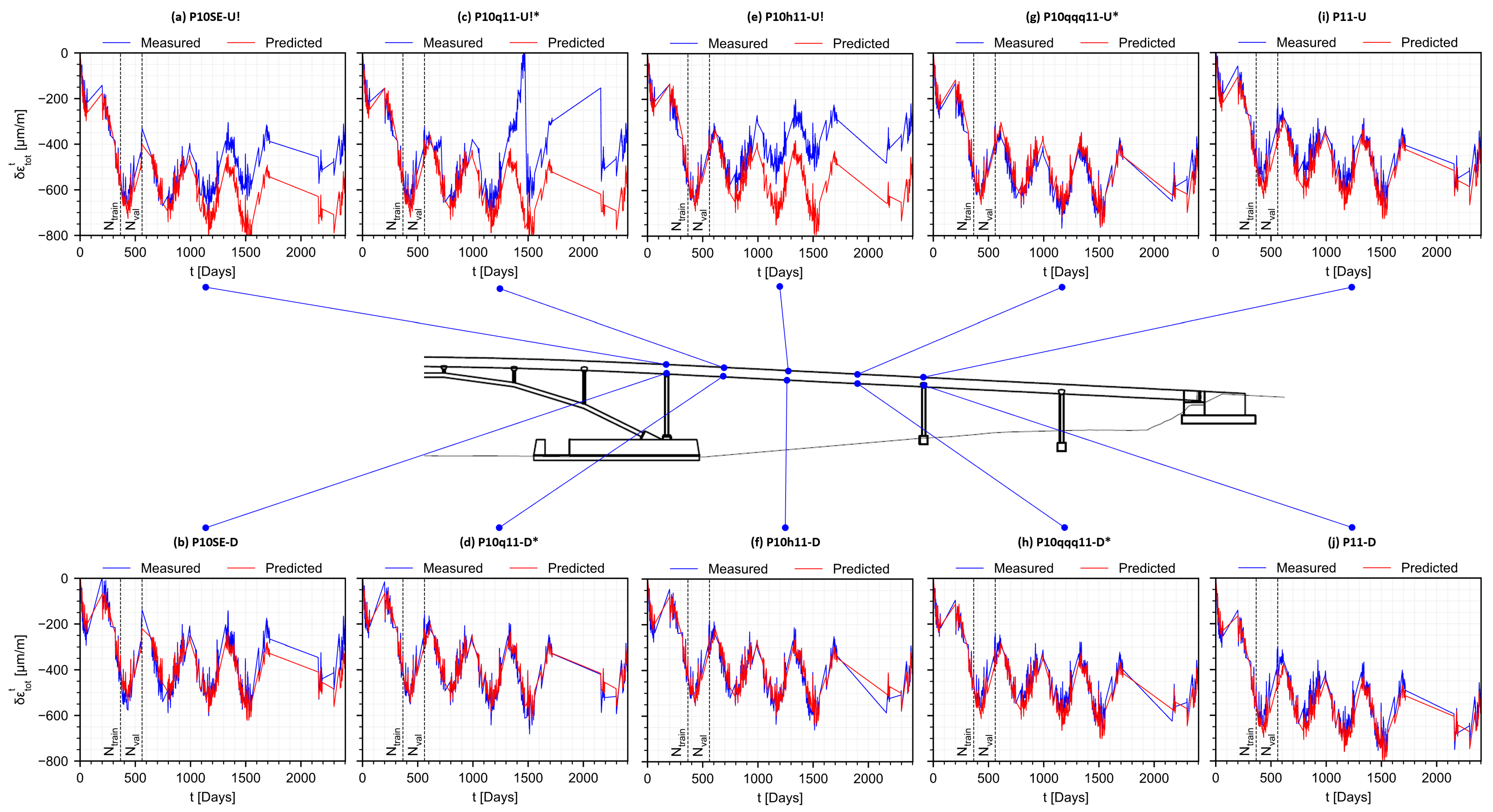
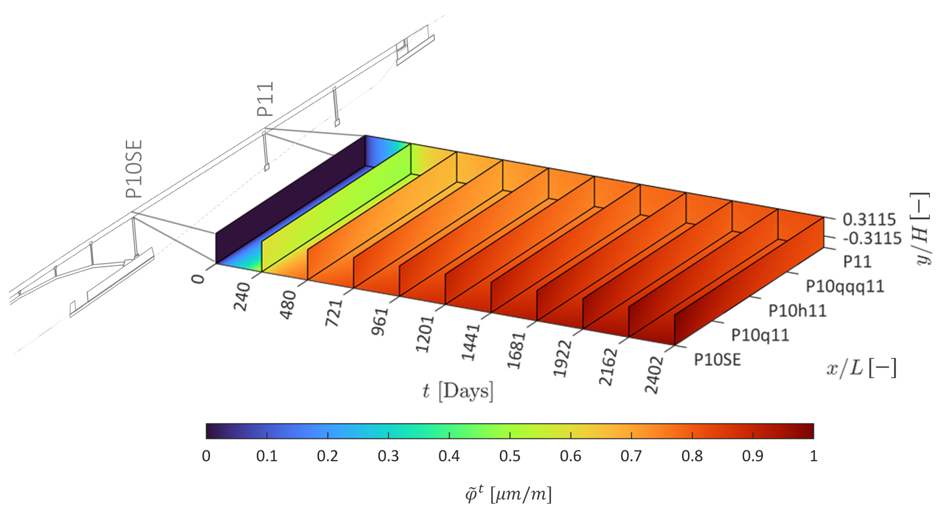
3. Results
4. Conclusions
Author Contributions
Funding
Institutional Review Board Statement
Informed Consent Statement
Data Availability Statement
Acknowledgments
Conflicts of Interest
Abbreviations
| MDPI | Multidisciplinary Digital Publishing Institute |
| FEM | Finite Element Method |
| SHM | Structural Health Monitoring |
| NN | Neural Networks |
| FOS | Fiber Optics Sensor |
| FBG | Fiber Bragg Grating |
| CNN | Convolutional Neural Networks |
| CTE | Coefficient of Thermal Expansion |
| FC | Fully Connected |
| RMSE | Root Mean Squared Error |
References
- Mehta, P.K.; Monteiro, P.J.M. Concrete Microstructure, Properties, and Materials; McGraw-Hill Education: New York, NY, USA, 2013. [Google Scholar]
- Bazant, Z.P.; Jirasek, M. Creep and Hygrothermal Effects in Concrete Structures; Springer: Dordrecht, The Netherlands, 2018. [Google Scholar]
- Dyer, T. Concrete Durability; CRC Press: Boca Raton, FL, USA, 2019. [Google Scholar]
- Melchers, R.E. Long-Term Durability of Marine Reinforced Concrete Structures. J. Mar. Sci. Eng. 2020, 8, 290. [Google Scholar] [CrossRef]
- Bonopera, M.; Chang, K.C.; Chen, C.C.; Lee, Z.K.; Sung, Y.C.; Tullini, N. Fiber Bragg Grating-Differential Settlement Measurement System for Bridge Displacement Monitoring: Case Study. J. Bridge Eng. 2019, 24, 05019011. [Google Scholar] [CrossRef]
- D’Altri, A.M.; Miranda, S.D.; Castellazzi, G.; Sarhosis, V.; Hudson, J.; Theodossopoulos, D. Historic Barrel Vaults Undergoing Differential Settlements. Int. J. Archit. Herit. 2020, 14, 1196–1209. [Google Scholar] [CrossRef]
- Ghorbani, E.; Svecova, D.; Thomson, D.J.; Cha, Y.J. Bridge pier scour level quantification based on output-only Kalman filtering. Struct. Health Monit. 2022, 21, 2116–2135. [Google Scholar] [CrossRef]
- Deng, L.; Cai, C.S. Bridge Scour: Prediction, Modeling, Monitoring, and Countermeasures—Review. Pract. Period. Struct. Des. Constr. 2010, 15, 125–134. [Google Scholar] [CrossRef]
- Glisic, B.; Inaudi, D.; Lau, J.; Fong, C. Ten-year monitoring of high-rise building columns using long-gauge fiber optic sensors. Smart Mater. Struct. 2013, 22, 055030. [Google Scholar] [CrossRef]
- Abdel-Jaber, H.; Glisic, B. Monitoring of long-term prestress losses in prestressed concrete structures using fiber optic sensors. Struct. Health Monit. 2019, 18, 254–269. [Google Scholar] [CrossRef]
- ACI Committee 209. Guide for Modeling and Calculating Shrinkage and Creep in Hardened Concrete. 2008. Available online: www.civil.northwestern.edu/people/bazant/PDFs/Backup%20of%20Papers/R21.pdf (accessed on 7 September 2022).
- CEB-FIP. CEB-FIP Model Code 1990: Design Code; Tomas Telford: London, UK, 1990. [Google Scholar]
- Gardner, N.; Lockman, M. Design provisions for drying shrinkage and creep of normal-strength concrete. ACI Mater. J. 2001, 98, 159–167. [Google Scholar]
- Hubler, M.; Wendner, R.; Bazant, Z. Statistical justification of model B4 for drying and autogenous shrinkage of concrete and comparisons to other models. Mater. Struct. 2015, 48, 797–814. [Google Scholar] [CrossRef]
- Al-Kamyani, Z.; Guadagnini, M.; Kypros, P. Predicting shrinkage induced curvature in plain and reinforced concrete. Eng. Struct. 2018, 176, 468–480. [Google Scholar] [CrossRef]
- Kaklauskas, G.; Gribniak, V. Eliminating Shrinkage Effect from Moment Curvature and Tension Stiffening Relationships of Reinforced Concrete Members. J. Struct. Eng. 2011, 137, 1460–1469. [Google Scholar] [CrossRef]
- Sousa, H.; Santos, L.; Chryssanthopoulous, M. Quantifying monitoring requirements for predicting creep deformations through Bayesian updating methods. Struct. Saf. 2019, 76, 40–50. [Google Scholar] [CrossRef]
- Joint ACI-ASCE Committee 423. Guide to Estimating Prestress Losses. 2016. Available online: https://www.doc88.com/p-18661732142167.html (accessed on 7 September 2022).
- Sousa, C.; Sousa, H.; Neves, A.S.; Figueiras, J. Numerical Evaluation of the Long-Term Behavior of Precast Continuous Bridge Decks. J. Bridge Eng. 2012, 17, 89–96. [Google Scholar] [CrossRef]
- Sousa, H.; Bento, J.; Figueiras, J. Construction assessment and long-term prediction of prestressed concrete bridges based on monitoring data. Eng. Struct. 2013, 52, 26–37. [Google Scholar] [CrossRef]
- Abdellatef, M.; Vorel, J.; Wan-Wendner, R.; Alnaggar, M. Predicting Time-Dependent Behavior of Post-Tensioned Concrete Beams: Discrete Multiscale Multiphysics Formulation. J. Struct. Eng. 2019, 145, 04019060. [Google Scholar] [CrossRef]
- Alnaggar, M.; Cusatis, G.; Di Luzio, G. Lattice Discrete Particle Modeling (LDPM) of Alkali Silica Reaction (ASR) deterioration of concrete structures. Cem. Concr. Compos. 2013, 41, 45–59. [Google Scholar] [CrossRef]
- Alnaggar, M.; Di Luzio, G.; Cusatis, G. Modeling Time-Dependent Behavior of Concrete Affected by Alkali Silica Reaction in Variable Environmental Conditions. Materials 2017, 10, 471. [Google Scholar] [CrossRef]
- Ghamsemzadeh, F.; Manafpour, A.; Sajedi, S.; Shekarchi, M.; Hatami, M. Predicting long-term compressive creep of concrete using inverse analysis method. Constr. Build. Mater. 2016, 124, 496–507. [Google Scholar] [CrossRef]
- Han, B.; Xiang, T.Y.; Xie, H.B. A Bayesian inference framework for predicting the long-term deflection of concrete structures causeed by creep and shrinkage. Eng. Struct. 2017, 142, 46–55. [Google Scholar] [CrossRef]
- Bal, L.; Buyle-Bodin, F. Artificial neural network for predicting drying shrinkage of concrete. Constr. Build. Mater. 2013, 38, 248–254. [Google Scholar] [CrossRef]
- Hauge, M. Machine Learning for Predictions of Strains Due to Long-Term Effects and Temperature in Concrete Structures. Master’s Thesis, Norwegian University of Sciente and Technology, Trondheim, Norway, 2019. [Google Scholar]
- Che, Z.; Purushotham, S.; Cho, K. Recurrent Neural Networks for Multivariate Time Series with Missing Values. Sci. Rep. 2018, 8, 6085. [Google Scholar] [CrossRef]
- Che, Z.; Purushotham, S.; Li, G.; Jiang, B.; Liu, Y. Hierarchical deep generative models for multi-rate multivariate time series. In Proceedings of the International Conference on Machine Learning, Stockholm, Sweden, 10–15 July 2018; Volume 80, pp. 784–793. [Google Scholar]
- Rubanova, Y.; Chen, R.T.Q.; Duvenaud, D.K. Latent Ordinary Differential Equations for Irregularly-Sampled Time Series. Adv. Neural Inf. Process. Syst. 2019, 32, 5320–5330. [Google Scholar]
- Oh, B.; Park, H.; Glisic, B. Prediction of long-term strain in concrete structure using convolutional neural networks, air temperature and time stamp of measurements. Autom. Constr. 2021, 126, 103665. [Google Scholar] [CrossRef]
- Karniadakis, G.; Levrelodos, I.; Lu, L.; Perdiaris, P.; Wang, S.; Yang, L. Physics-informed machine learning. Nat. Rev. Phys. 2021, 3, 422–440. [Google Scholar] [CrossRef]
- Sigurdardottir, D.; Glisic, B. On-Site Validation of Fiber-Optic Methods for Structural Health Monitoring: Streicker Bridge. J. Civ. Struct. Health Monit. 2015, 5, 529–549. [Google Scholar] [CrossRef]
- Glisic, B. CEE 537 Structural Health Monitoring, Graduate Course. 2019. Available online: https://cee.princeton.edu/people/branko-glisic (accessed on 7 September 2022).
- Pereira, M.; Glisic, B. A hybrid approach for prediction of long-term behavior of concrete structures. J. Civ. Struct. Health Monit. 2022, 12, 891–911. [Google Scholar] [CrossRef]
- Montavon, G.; Orr, G.; Muller, K.R. Neural Networks: Tricks of the Trade; Springer: Berlin/Heidelberg, Germany, 2012. [Google Scholar]
- Kingma, D.; Ba, J. Adam: A method for stochastic optimization. In Proceedings of the 3rd International Conference for Learning Representations, San Diego, CA, USA, 7–9 May 2015. [Google Scholar]


| Property | Value |
|---|---|
| Strain uncertainty | 2 µm/m |
| Temperature uncertainty | 0.2 C |
| Typical gauge length | 60 cm |
| Dynamic range | −5000 to +7500 µm/m |
| Max. sampling frequency | 250 Hz |
| [C] | [µm/m] | |||||
|---|---|---|---|---|---|---|
| Position | Train | Val. | Test | Train | Val. | Test |
| P10SE-U | 1.5 | 1.2 | 2.6 | 23.0 | 49.5 | 124.2 |
| P10SE-D | 1.1 | 1.3 | 2.7 | 33.0 | 38.9 | 51.4 |
| P10q11-U * | 2.5 | 2.1 | 13.8 | 27.2 | 48.3 | 174.9 |
| P10q11D * | 1.0 | 1.3 | 2.1 | 20.0 | 26.3 | 27.8 |
| P10h11-U | 1.3 | 2.1 | 2.7 | 34.9 | 22.1 | 174.5 |
| P10h11D | 0.9 | 1.0 | 2.2 | 23.0 | 27.6 | 27.1 |
| P10qqq11-U * | 1.5 | 2.1 | 2.5 | 37.0 | 18.7 | 36.9 |
| P10qqq11D * | 1.0 | 1.2 | 2.4 | 14.3 | 47.4 | 36.6 |
| P11-U | 1.0 | 1.5 | 2.5 | 29.2 | 67.8 | 49.0 |
| P11D | 1.0 | 1.1 | 2.3 | 21.7 | 59.5 | 41.6 |
Publisher’s Note: MDPI stays neutral with regard to jurisdictional claims in published maps and institutional affiliations. |
© 2022 by the authors. Licensee MDPI, Basel, Switzerland. This article is an open access article distributed under the terms and conditions of the Creative Commons Attribution (CC BY) license (https://creativecommons.org/licenses/by/4.0/).
Share and Cite
Pereira, M.; Glisic, B. Physics-Informed Data-Driven Prediction of 2D Normal Strain Field in Concrete Structures. Sensors 2022, 22, 7190. https://doi.org/10.3390/s22197190
Pereira M, Glisic B. Physics-Informed Data-Driven Prediction of 2D Normal Strain Field in Concrete Structures. Sensors. 2022; 22(19):7190. https://doi.org/10.3390/s22197190
Chicago/Turabian StylePereira, Mauricio, and Branko Glisic. 2022. "Physics-Informed Data-Driven Prediction of 2D Normal Strain Field in Concrete Structures" Sensors 22, no. 19: 7190. https://doi.org/10.3390/s22197190
APA StylePereira, M., & Glisic, B. (2022). Physics-Informed Data-Driven Prediction of 2D Normal Strain Field in Concrete Structures. Sensors, 22(19), 7190. https://doi.org/10.3390/s22197190