
ResNet-AE for Radar Signal Anomaly Detection

Abstract
:1. Introduction
- An anomaly detection method based on ResNet-AE is proposed to detect radar signal time-series data.
- Our method is jointly ResNet and autoencoder, which takes good feature extraction and reconstruction capabilities.
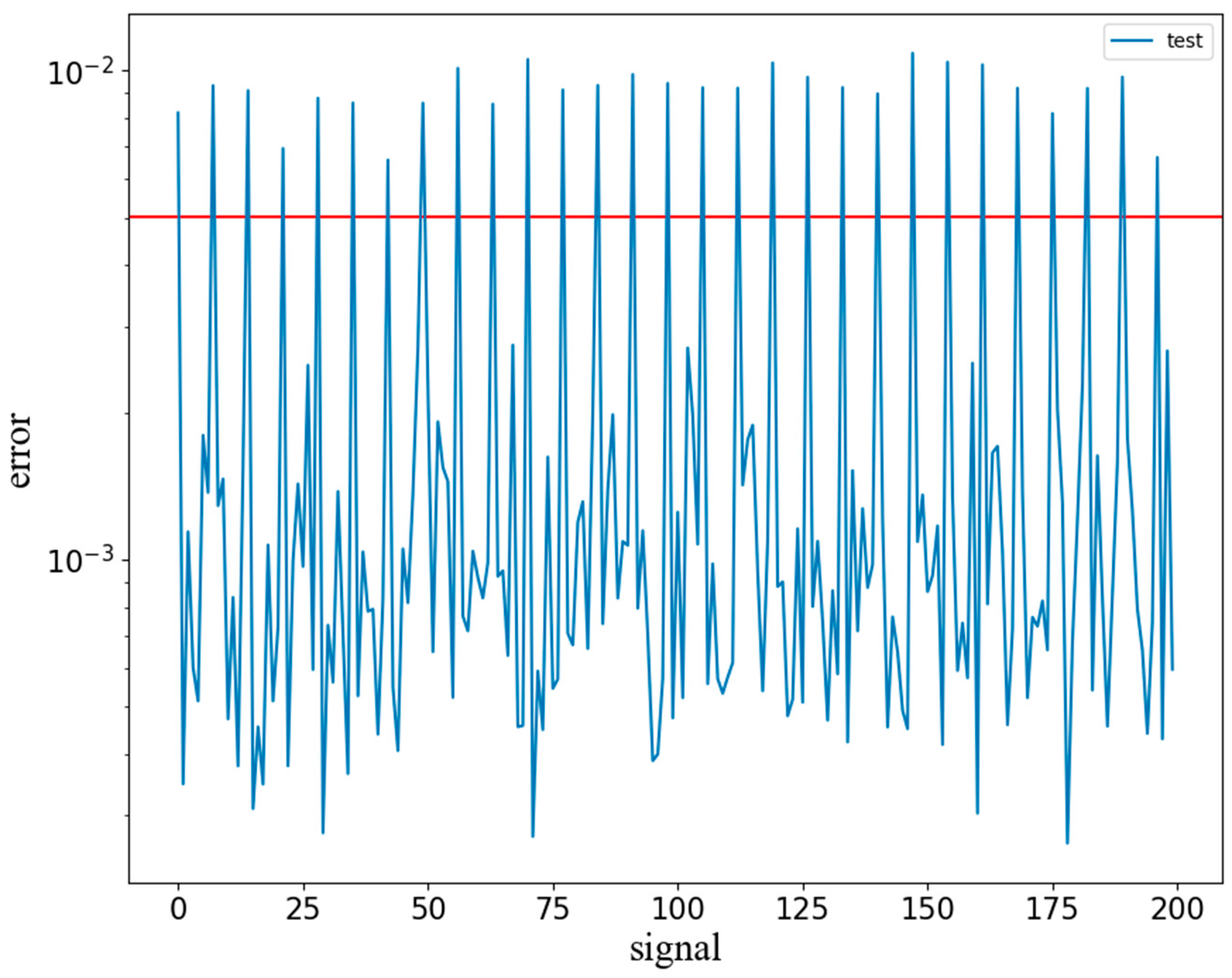
- Anomaly score is an adaptive threshold obtained by clustering the reconstructed difference, which makes it more able to distinguish anomalies from normal data.
2. ResNet-AE Anomaly Detection Model
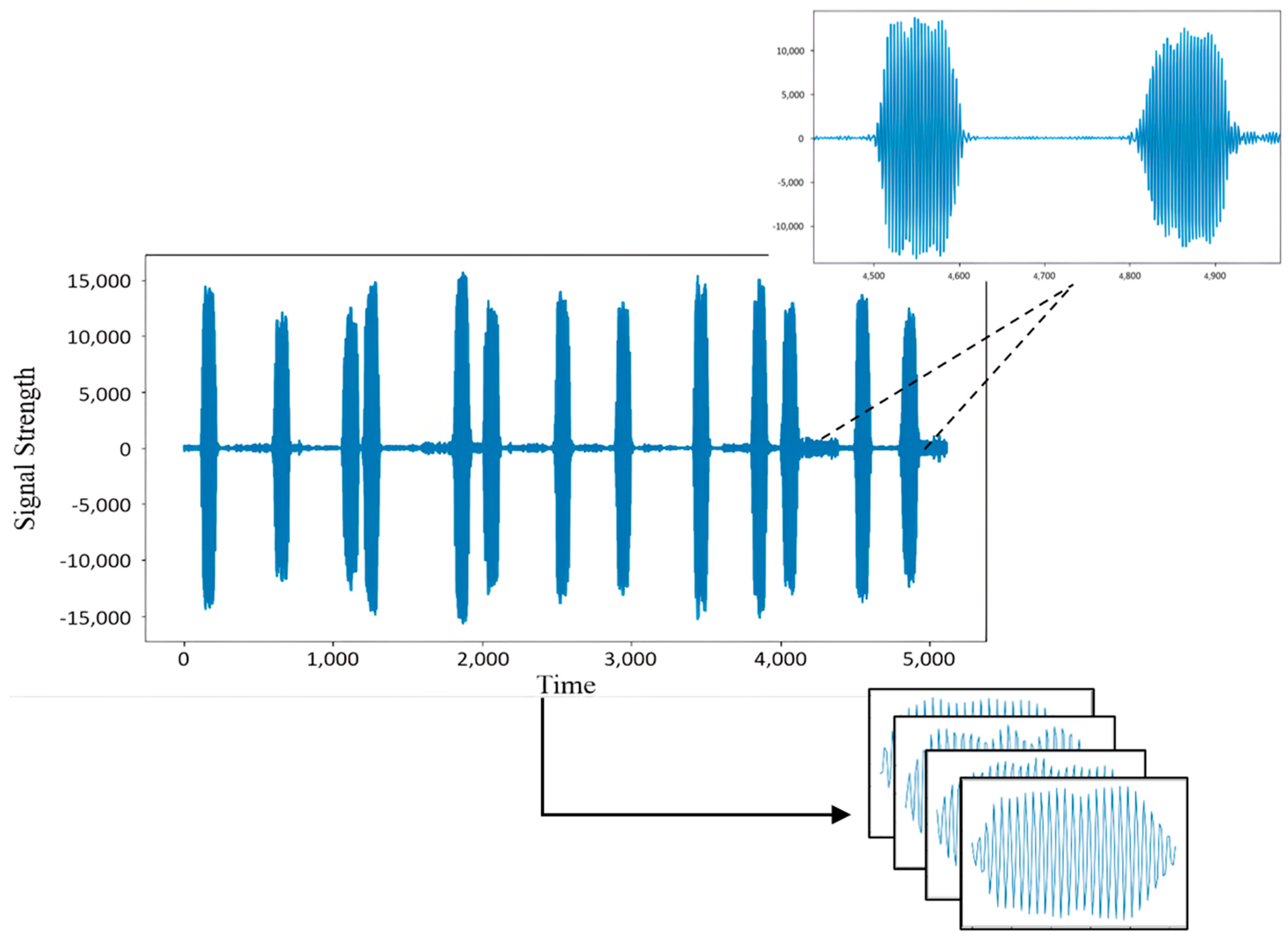
2.1. Dataset
2.2. Model Construction and Training
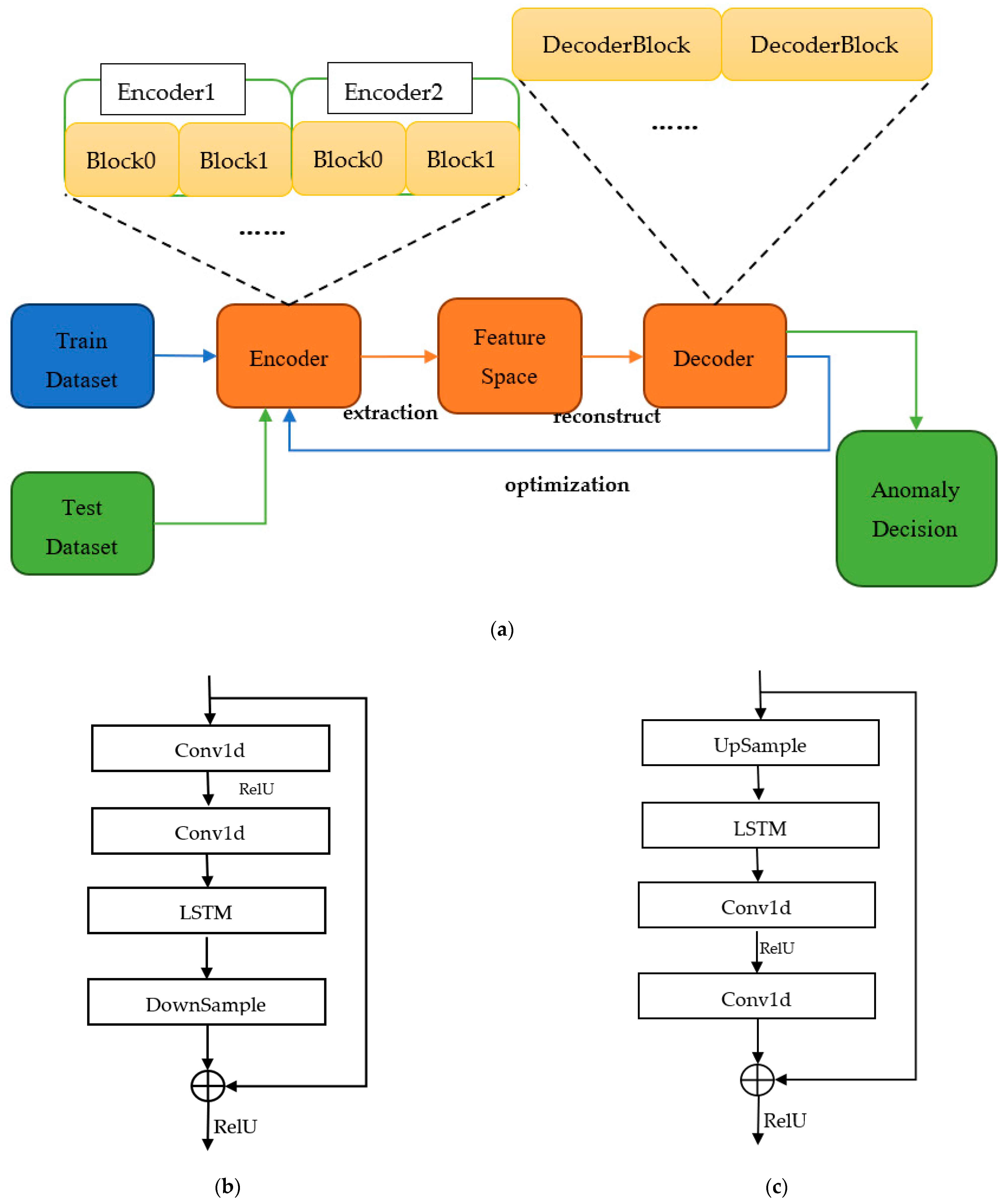
2.2.1. Network Structure
2.2.2. ResNet-AE
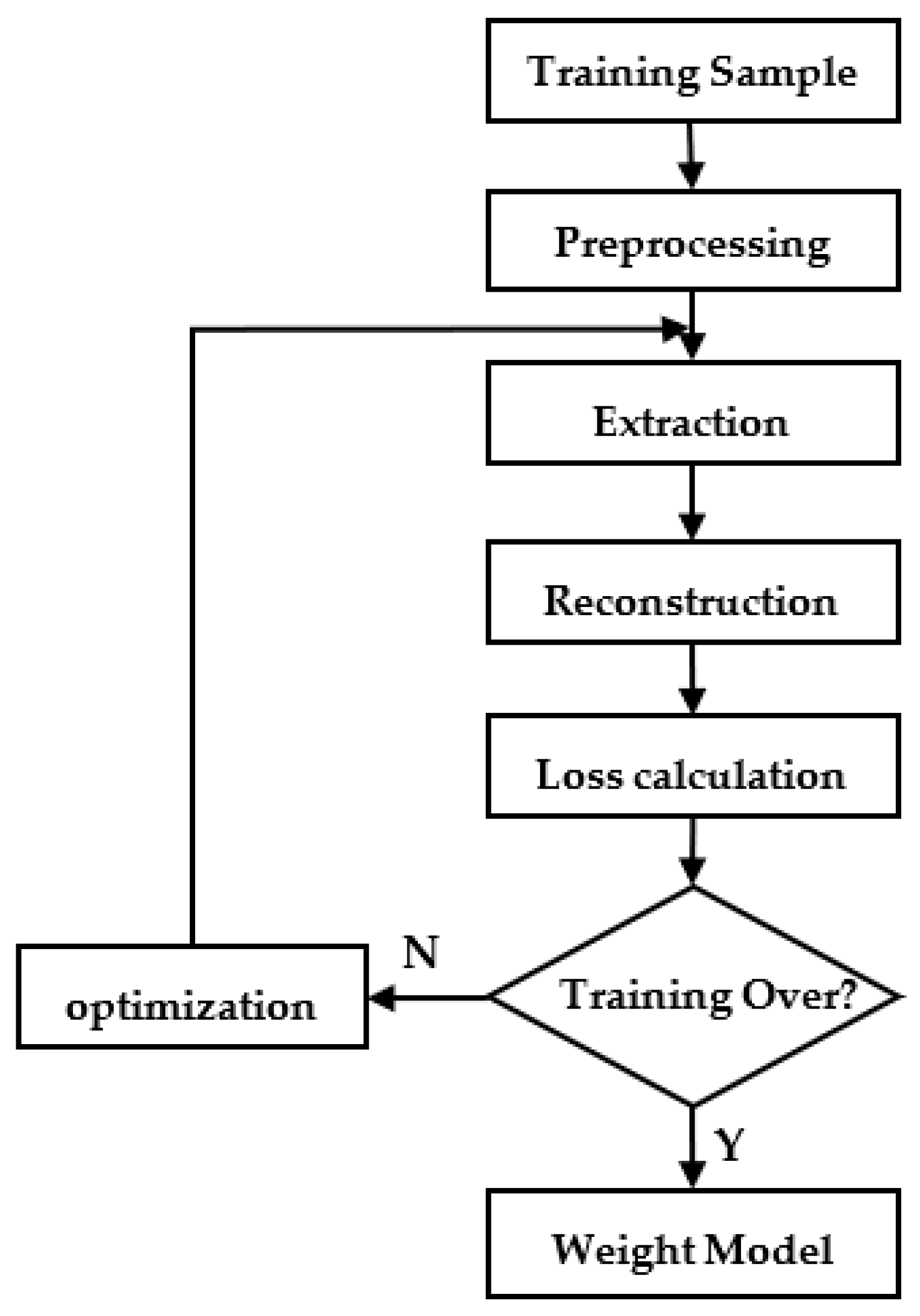
2.3. Training Process
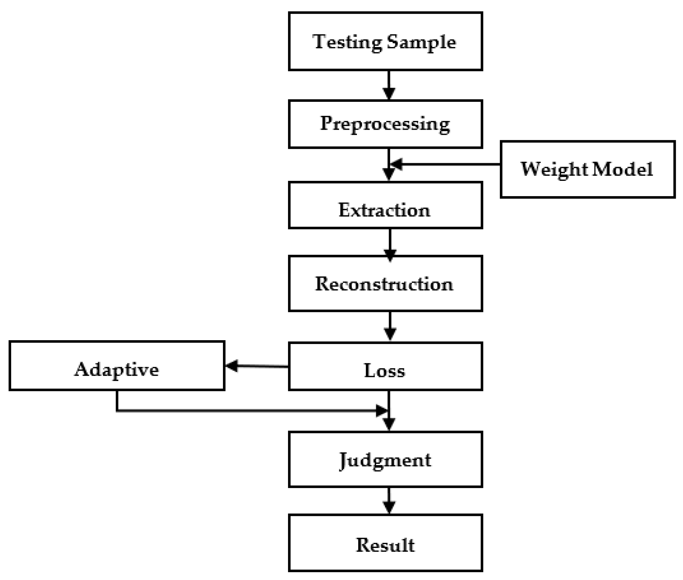
2.4. Anomaly Decision
3. Experiment
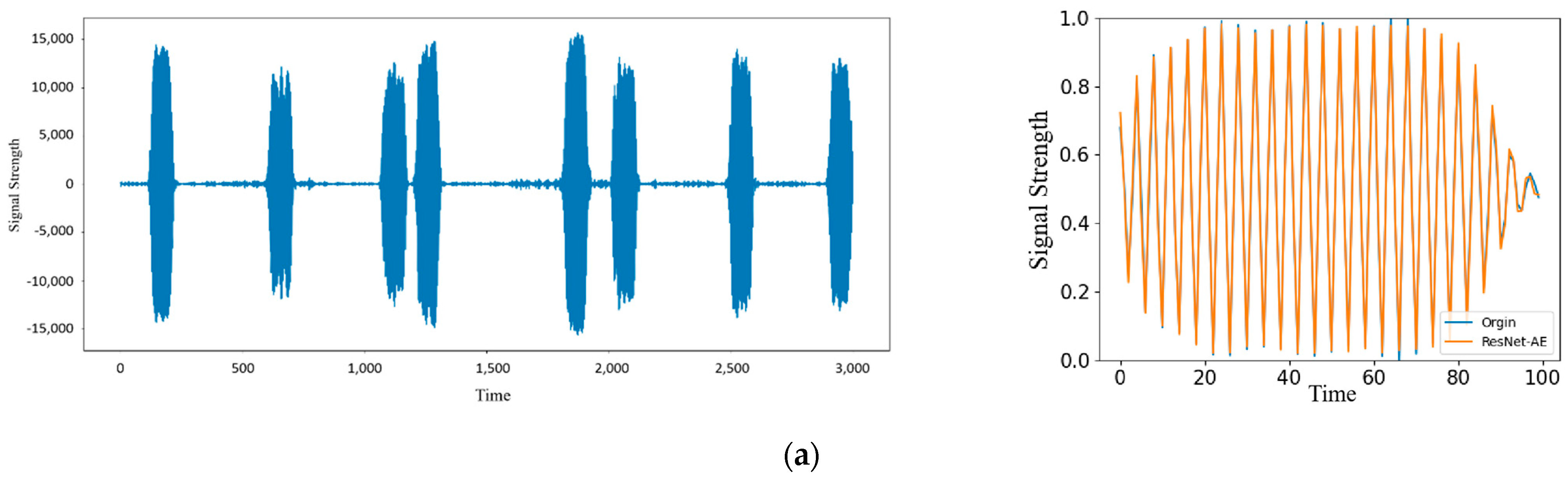
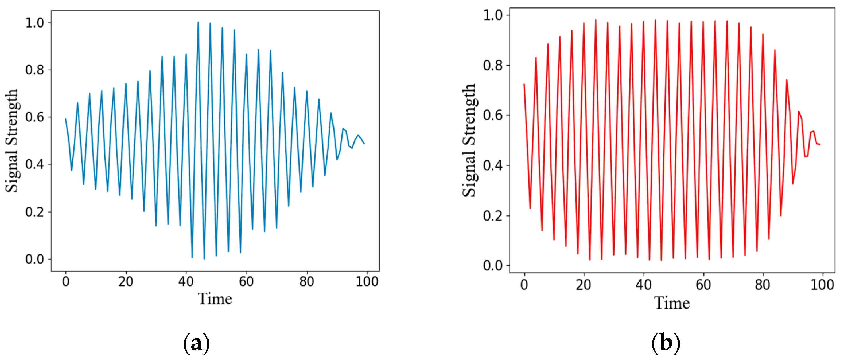
3.1. Data Preprocessing
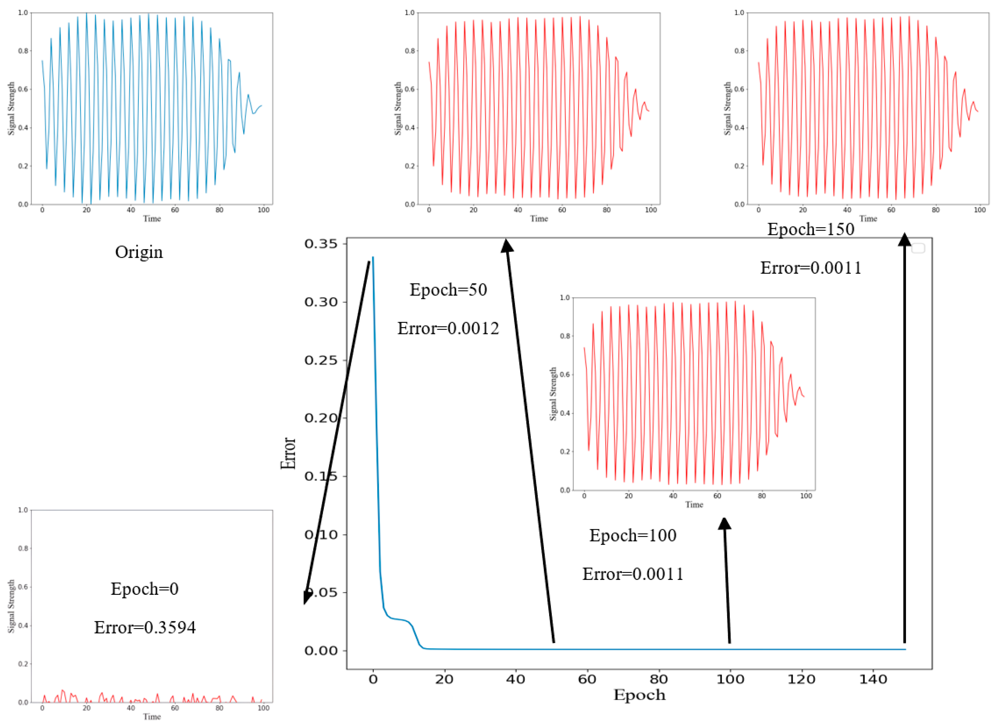
3.2. Model Training
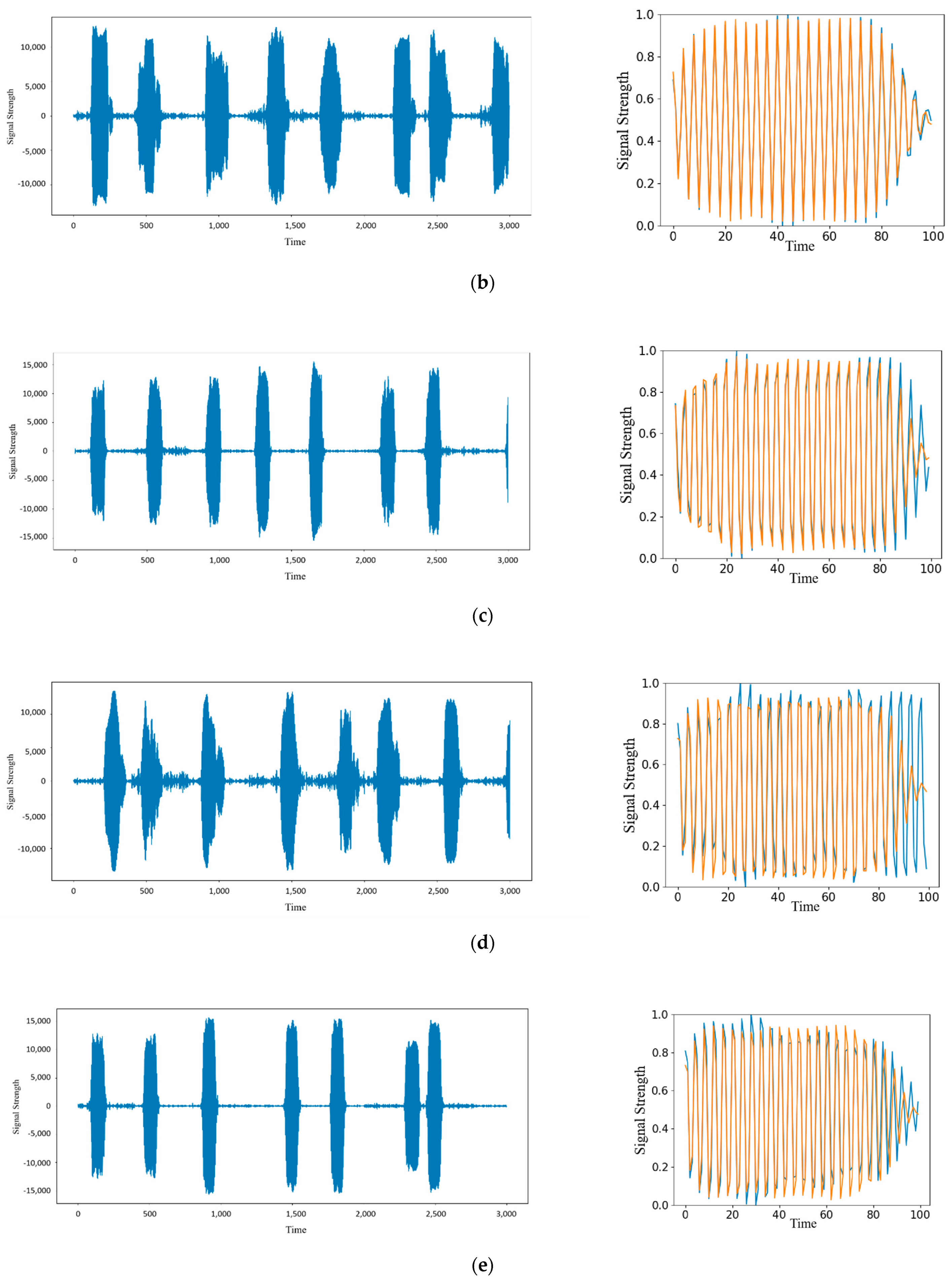
3.3. Model Testing
3.4. Model Evaluation
4. Results and Analysis
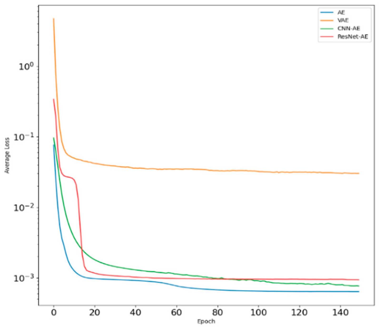
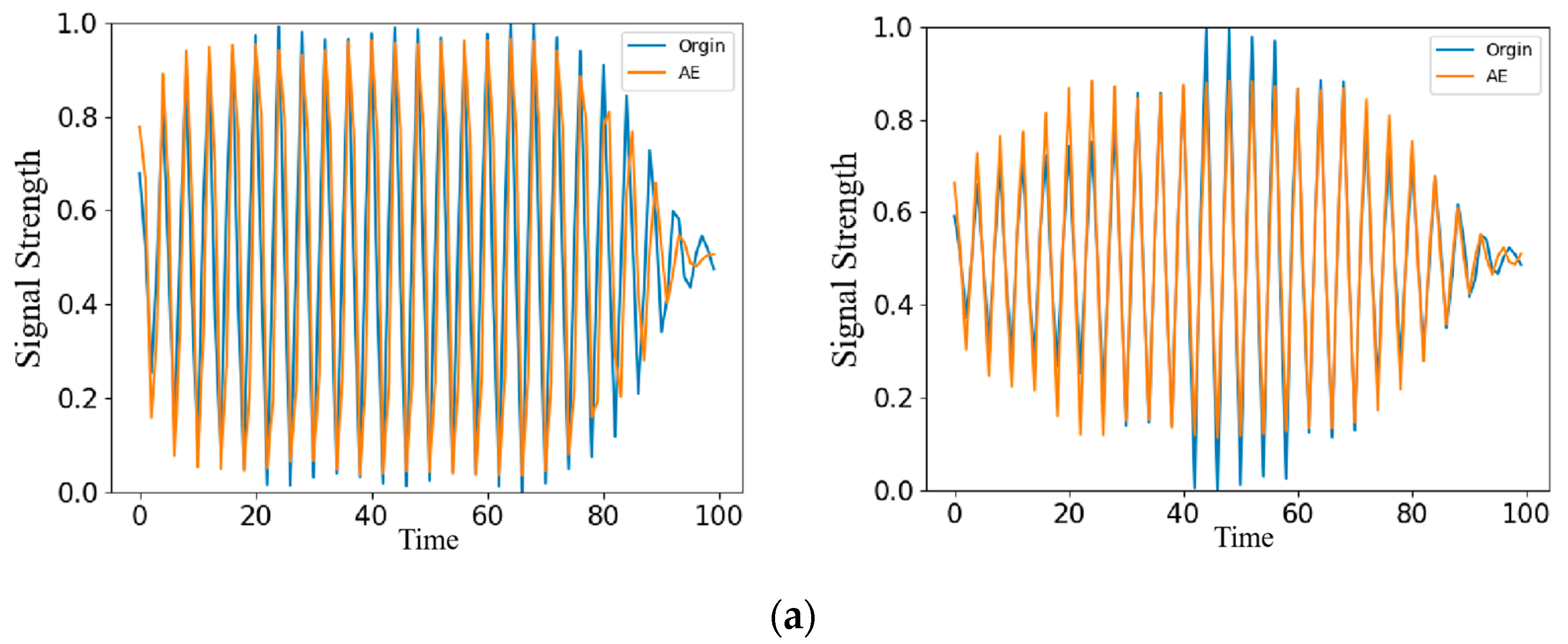
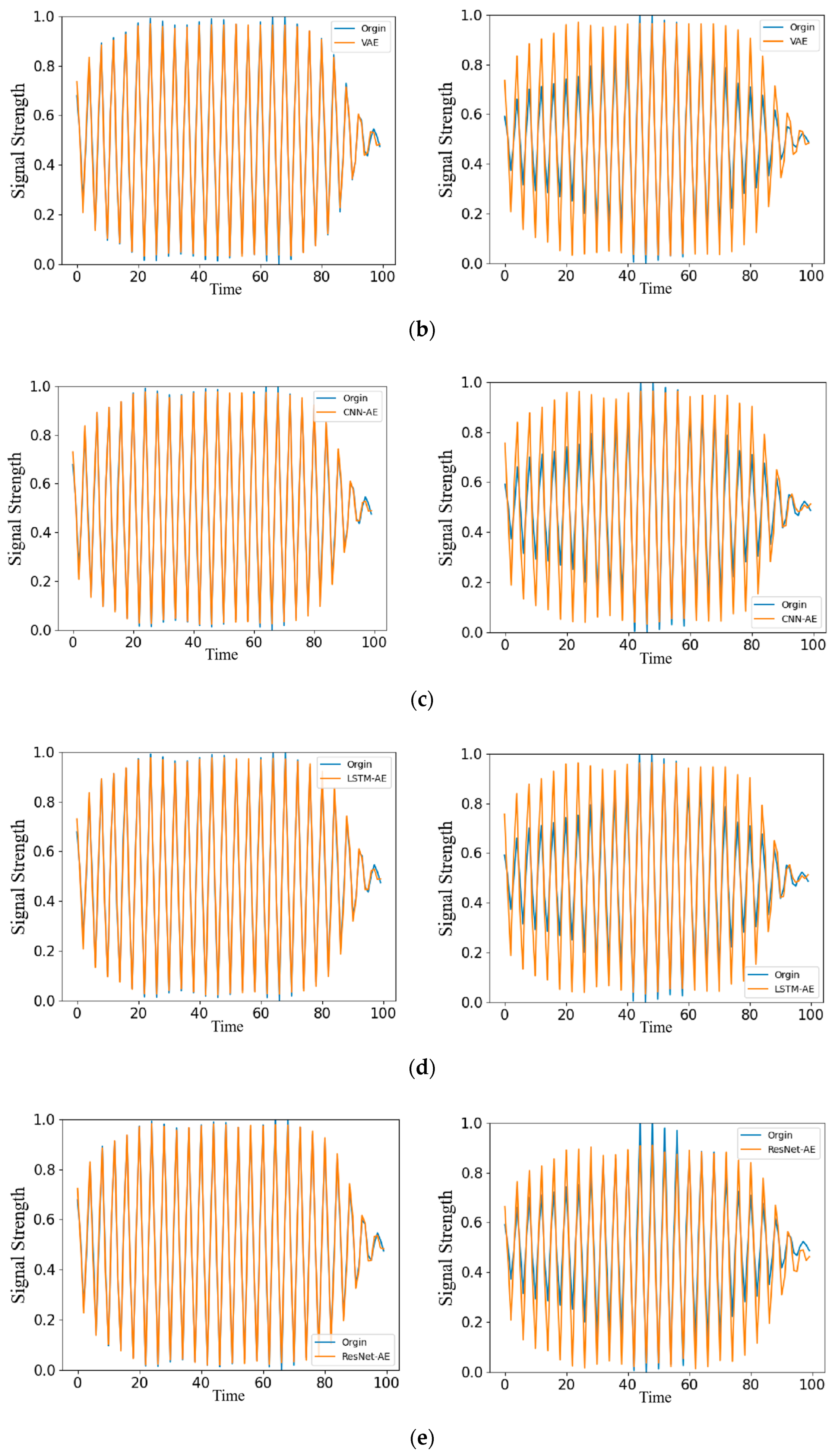
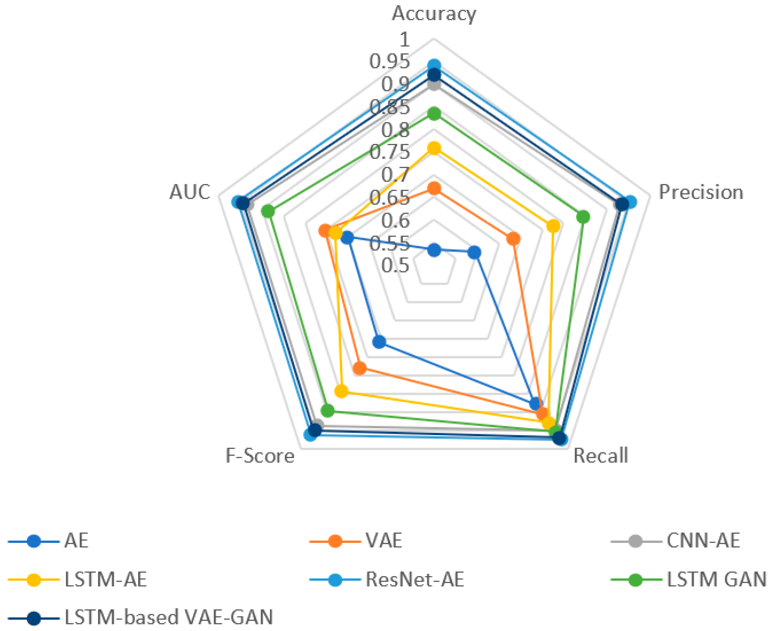
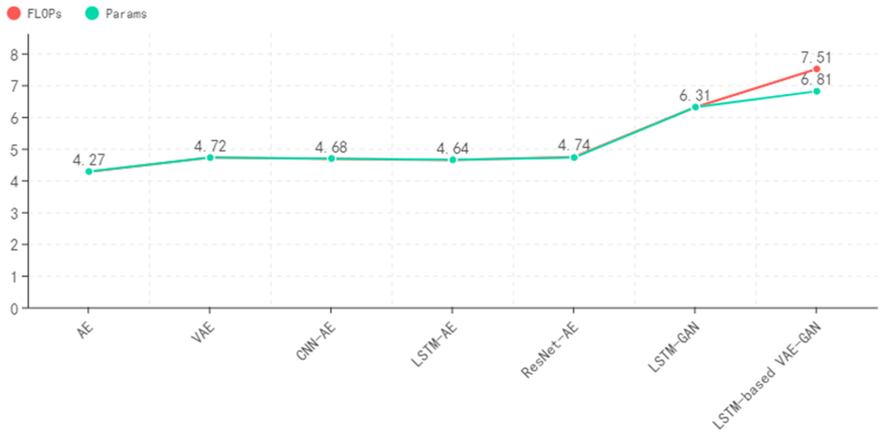
4.1. Comparison of Common Models
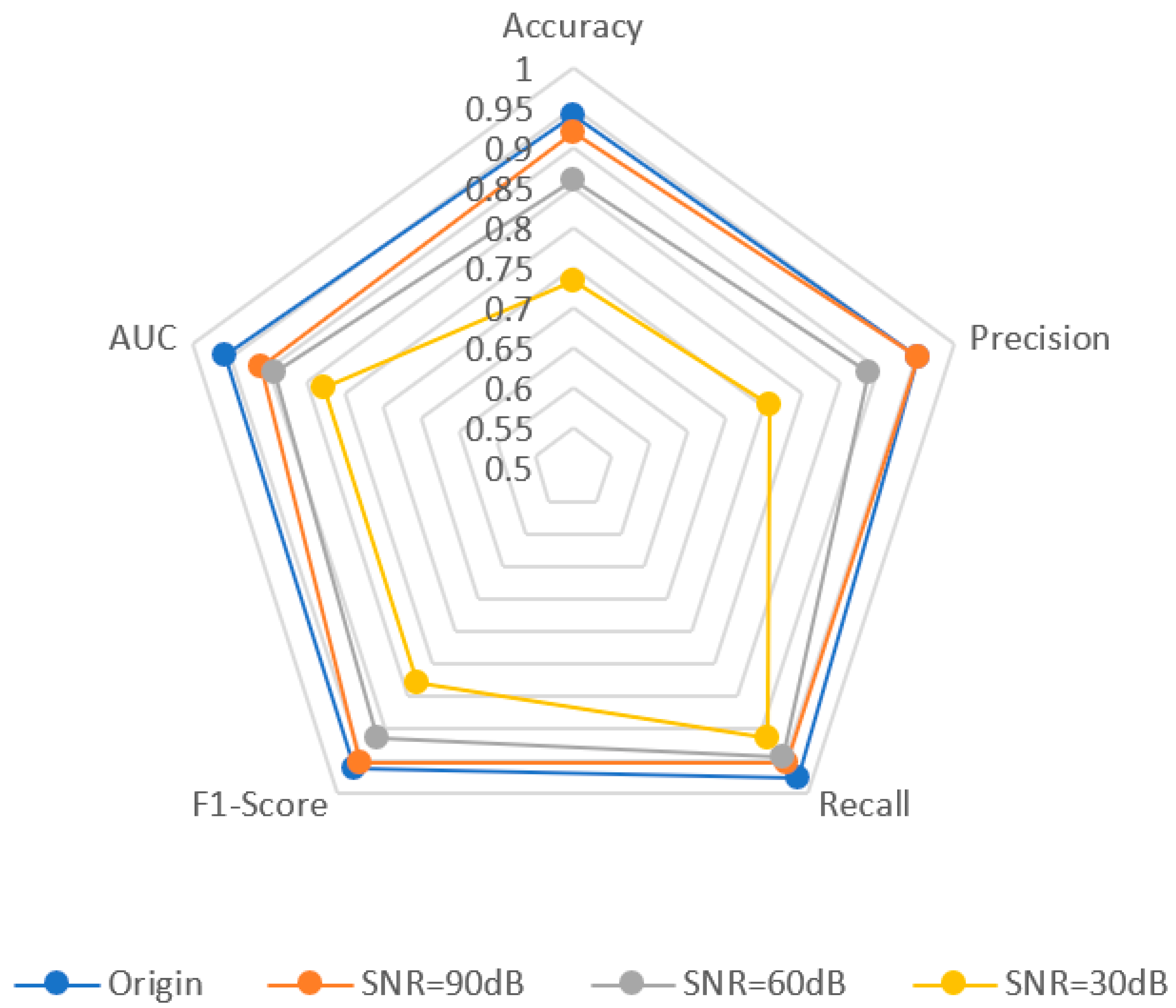
4.2. Influence of SNR
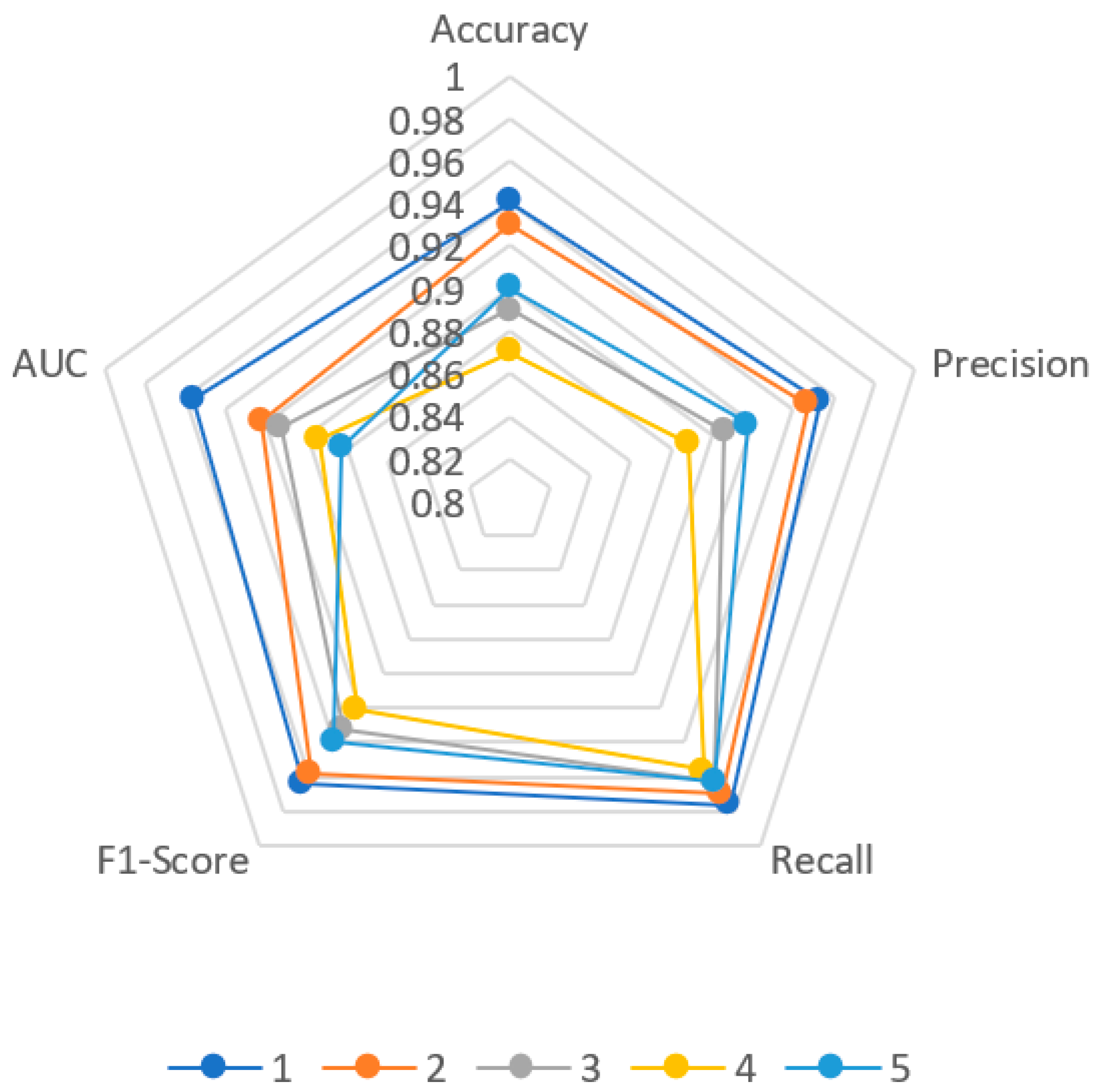
4.3. Generality Analysis
5. Conclusions
Author Contributions
Funding
Institutional Review Board Statement
Informed Consent Statement
Data Availability Statement
Conflicts of Interest
References
- Yang, C.B. Research on Anomaly Detection Method of Electromagnetic Environment Based on Deep Learning; Harbin Engineering University: Harbin, China, 2020. [Google Scholar]
- Chandola, V.; Banerjee, A.; Kumar, V. Anomaly Detection: A Survey. ACM Comput. Surv. 2009, 41, 1–58. [Google Scholar] [CrossRef]
- Hojjati, H.; Ho, T.; Armanfard, N. Self-Supervised Anomaly Detection: A Survey and Outlook. arXiv 2022, arXiv:2205.05173. [Google Scholar]
- Habeeb, R.A.A.; Nasaruddin, F.; Gani, A.; Hashem, I.A.T.; Ahmed, E.; Imran, M. Real-time big data processing for anomaly detection: A Survey. Int. J. Inf. Manag. 2018, 45, 289–307. [Google Scholar] [CrossRef]
- Ramaswamy, S.; Rastogi, R.; Shim, K. Efficient Algorithms for Mining Outliers from Large Data Sets. In Proceedings of the International Conference on Management of Data, Dallas, TX, USA, 15–18 May 2000; ACM: New York, NY, USA, 2000. [Google Scholar]
- Breunig, M.M.; Kriegel, H.P.; Ng, R.T.; Sander, J. LOF: Identifying Density-Based Local Outliers. In Proceedings of the 2000 ACM SIGMOD International Conference on Management of Data, Dallas, TX, USA, 15–18 May 2000. [Google Scholar]
- Erfani, S.M.; Rajasegarar, S.; Karunasekera, S.; Leckie, C. High-dimensional and large-scale anomaly detection using a linear one-class SVM with deep learning. Pattern Recognit. 2016, 58, 121–134. [Google Scholar] [CrossRef]
- Maimó, L.F.; Gómez, Á.L.P.; Clemente, F.J.G.; Pérez, M.G.; Pérez, G.M. A Self-Adaptive Deep Learning-Based System for Anomaly Detection in 5G Networks. IEEE Access 2018, 6, 7700–7712. [Google Scholar] [CrossRef]
- Wang, X.; Zhou, Q.; Harer, J.; Brown, G.; Qiu, S.; Dou, Z.; Wang, J.; Hinton, A.; Aguayo, C.; Chin, P. Deep Learning-Based Classification and Anomaly Detection of Side-Channel Signals. In Proceedings of the SPIE DEFENSE + SECURITY, Orlando, FL, USA, 15–19 April 2018; SPIE: Washington, DC, USA, 2018. [Google Scholar]
- An, J.; Cho, S. Variational Autoencoder Based Anomaly Detection Using Reconstruction Probability. Spec. Lect. IE 2015, 2, 1–18. [Google Scholar]
- O’Shea, T.J.; Clancy, T.C.; Mcgwier, R.W. Recurrent Neural Radio Anomaly Detection. arXiv 2016, arXiv:1611.00301. [Google Scholar]
- Xu, H.; Chen, W.; Zhao, N.; Li, Z.; Bu, J.; Li, Z.; Liu, Y.; Zhao, Y.; Pei, D.; Qiao, H.; et al. Unsupervised Anomaly Detection Via Variational Auto-Encoder for Seasonal KPIs in Web Applications. In Proceedings of the 2018 World Wide Web Conference, Lyon, France, 23–27 April 2018; Republic and Canton of Geneva: International World Wide Web Conferences Steering Committee, 2018; pp. 187–196. [Google Scholar]
- Chen, W.; Xu, H.; Li, Z.; Pei, D.; Chen, J.; Qiao, H.; Feng, Y.; Wang, Z. Unsupervised Anomaly Detection for Intricate KPIs via Adversarial Training of VAE. In Proceedings of the IEEE Conference on Computer Communications, Paris, France, 29 April–2 May 2019; IEEE Press: Piscataway, NJ, USA, 2019; pp. 1891–1899. [Google Scholar]
- Niu, Z.J.; Yu, K.; Wu, X.F. LSTM-based VAE-GAN for time-series anomaly detection. Sensors 2020, 20, 3738. [Google Scholar] [CrossRef]
- Lin, S.; Clark, R.; Birke, R.; Schonborn, S.; Trigoni, N.; Roberts, S. Anomaly Detection for Time Series Using VAE-LSTM Hybrid Model. In Proceedings of the ICASSP 2020–2020 IEEE International Conference on Acoustics, Speech and Signal Processing (ICASSP), Barcelona, Spain, 4–8 May 2020; pp. 4322–4326. [Google Scholar] [CrossRef]
- Audibert, J.; Guyard, F.; Marti, S.; Zuluaga, M. USAD: Unsupervised Anomaly Detection on Multivariate Time Series. In Proceedings of the 26th ACM SIGKDD International Conference on Knowledge Discovery & Data Mining, Virtual Event, CA, USA, 6–10 July 2020; pp. 3395–3404. [Google Scholar] [CrossRef]
- Xunhua, H.; Fengbin, Z.; Haoyi, F.; Liang, X. Multimodal Adversarial Learning Based Unsupervised Time Series Anomaly Detection on. Comput. Res. Dev. 2021, 58, 1655–1667. [Google Scholar]
- Wu, Z.; Shen, C.; Van Den Hengel, A. Wider or deeper: Revisiting the resnet model for visual recognition. Pattern Recog. 2019, 90, 119–133. [Google Scholar] [CrossRef]
- Lopez, R.; Regier, J.; Jordan, M.I.; Yosef, N. Information Constraints on Auto-Encoding Variational Bayes. In Proceedings of the Advances in Neural Information Processing Systems 31 (NeurIPS 2018), Montréal, QC, Canada, 3–8 December 2018. [Google Scholar]
- He, K.; Zhang, X.; Ren, S.; Sun, J. Deep Residual Learning for Image Recognition. In Proceedings of the 2016 IEEE Conference on Computer Vision and Pattern Recognition (CVPR), Las Vegas, NV, USA, 27–30 June 2016; pp. 770–778. [Google Scholar] [CrossRef]
- Liu, Y.; Li, Z.; Zhou, C.; Jiang, Y.; Sun, J.; Wang, M.; He, X. Generative Adversarial Active Learning for Unsupervised Outlier Detection. IEEE Trans. Knowl. Data Eng. 2019, 99, 1. [Google Scholar] [CrossRef]
- Gupta, M.; Gao, J.; Aggarwal, C.C.; Han, J. Outlier Detection for Temporal Data: A Survey. IEEE Trans. Knowl. Data Eng. 2014, 26, 2250–2267. [Google Scholar] [CrossRef]
- Lee, S.; Park, G.; Park, J. Daily Behavior Pattern Extraction using Time-Series Behavioral Data of Dairy Cows and k-Means Clustering. J. Softw. Assess. Valuat. 2021, 17, 83–92. [Google Scholar] [CrossRef]
- Ro, K.; Zou, C.; Wang, Z.; Yin, G. Outlier detection for high-dimensional data. Biometrika 2015, 102, 589–599. [Google Scholar] [CrossRef]
- Garg, A.; Zhang, W.; Samaran, J.; Savitha, R.; Foo, C.-S. An Evaluation of Anomaly Detection and Diagnosis in Multivariate Time Series. IEEE Trans. Neural Netw. Learn. Syst. 2021, 33, 2508–2517. [Google Scholar] [CrossRef] [PubMed]
- Park, D.; Hoshi, Y.; Kemp, C.C. A Multimodal Anomaly Detector for Robot-Assisted Feeding Using an LSTM-Based Variational Autoencoder. IEEE Robot. Autom. Lett. 2018, 3, 1544–1551. [Google Scholar] [CrossRef]
- Malhotra, P.; Ramakrishnan, A.; Anand, G.; Vig, L.; Agarwal, P.; Shroff, G. LSTM-based encoder-decoder for multi-sensor anomaly detection. arXiv 2016, arXiv:1607.00148. [Google Scholar]
- Song, Q. Deep Autoencoding Gaussian Mixture Model for Unsupervised Anomaly Detection. In Proceedings of the International Conference on Learning Representations, Vancouver, BC, Canada, 30 April–3 May 2018. [Google Scholar]
- Schlegl, T.; Seeböck, P.; Waldstein, S.M.; Langs, G.; Schmidt-Erfurth, U. f-AnoGAN: Fast Unsupervised Anomaly Detection with Generative Adversarial Networks. Med. Image Anal. 2019, 56, 30–44. [Google Scholar] [CrossRef] [PubMed]
- Dan, L. Anomaly Detection with Generative Adversarial Networks for Multivariate Time Series. In Proceedings of the 7th International Workshop on Big Data, Streams and Heterogeneous Source Mining: Algorithms, Systems, Programming Models and Applications on the ACM Knowledge Discovery and Data Mining Conference, London, UK, 4–8 August 2018; ACM: New York, NY, USA, 2018. [Google Scholar]
- Andrey, Y.L. Real-time Anomaly Detection and Classification in Streaming PMU Data. arXiv 2019, arXiv:1911.06316. [Google Scholar]
- Zhang, J.Y.; Yang, W.J. Research on network traffic classification and recognition based on deep learning. J. Tianjin Univ. Technol. 2019, 6, 35–40. [Google Scholar]


| Hardware or Software | Technical Parameter | Hardware or Software |
|---|---|---|
| Operation System | Windows 10 Home Chinese | Operation System |
| CPU | Intel Core i5-10300H | CPU |
| GPU | NVIDIA Geforce RTX 2060 | GPU |
| Memory | 32 G | Memory |
| Python | Python 3.8.5 | Python |
| Pytorch | Pytorch 1.6.0 | Pytorch |
| Hyperparameter | |
|---|---|
| Batch size | 64 |
| Epochs | 150 |
| Learning rate | 0.001 |
| Loss function | MSE |
| Optimizer | Adam |
Publisher’s Note: MDPI stays neutral with regard to jurisdictional claims in published maps and institutional affiliations. |
© 2022 by the authors. Licensee MDPI, Basel, Switzerland. This article is an open access article distributed under the terms and conditions of the Creative Commons Attribution (CC BY) license (https://creativecommons.org/licenses/by/4.0/).
Share and Cite
Cheng, D.; Fan, Y.; Fang, S.; Wang, M.; Liu, H. ResNet-AE for Radar Signal Anomaly Detection. Sensors 2022, 22, 6249. https://doi.org/10.3390/s22166249
Cheng D, Fan Y, Fang S, Wang M, Liu H. ResNet-AE for Radar Signal Anomaly Detection. Sensors. 2022; 22(16):6249. https://doi.org/10.3390/s22166249
Chicago/Turabian StyleCheng, Donghang, Youchen Fan, Shengliang Fang, Mengtao Wang, and Han Liu. 2022. "ResNet-AE for Radar Signal Anomaly Detection" Sensors 22, no. 16: 6249. https://doi.org/10.3390/s22166249
APA StyleCheng, D., Fan, Y., Fang, S., Wang, M., & Liu, H. (2022). ResNet-AE for Radar Signal Anomaly Detection. Sensors, 22(16), 6249. https://doi.org/10.3390/s22166249