
Air Pollution Detection Using a Novel Snap-Shot Hyperspectral Imaging Technique


Abstract
:1. Introduction
2. Materials and Methods
2.1. Dataset
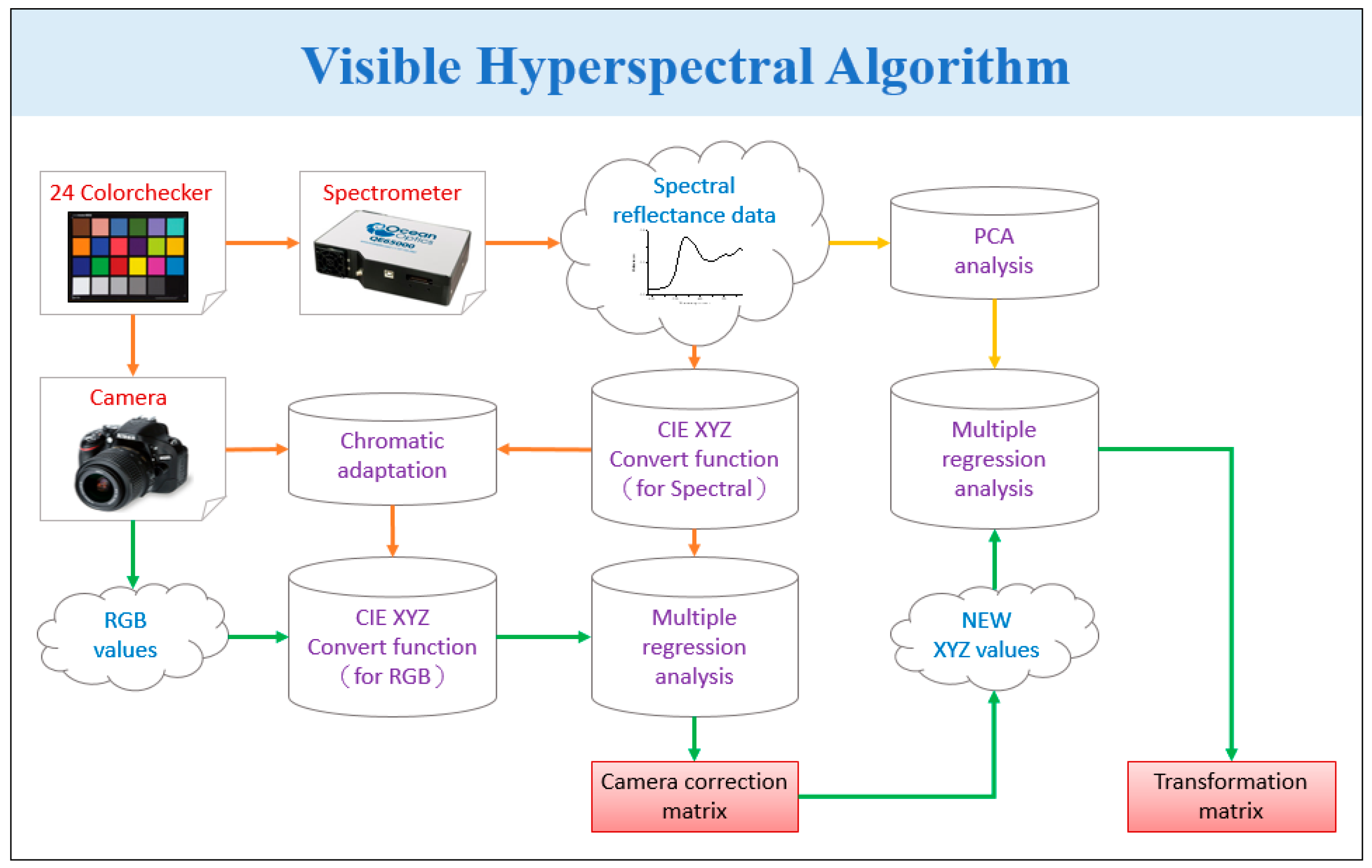
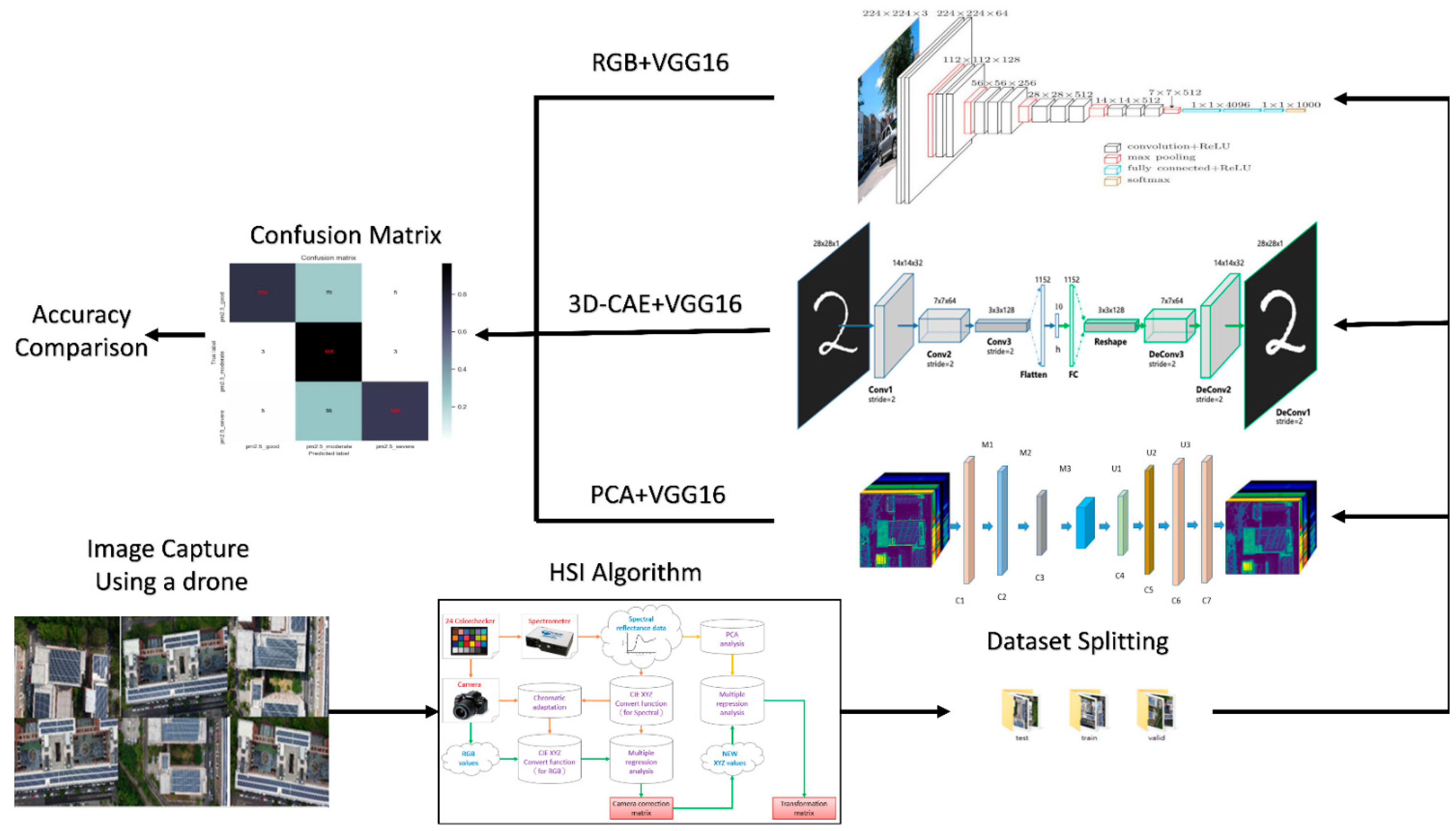
2.2. HSI Algorithm
2.3. Three-Dimensional-Convolution Auto Encoder
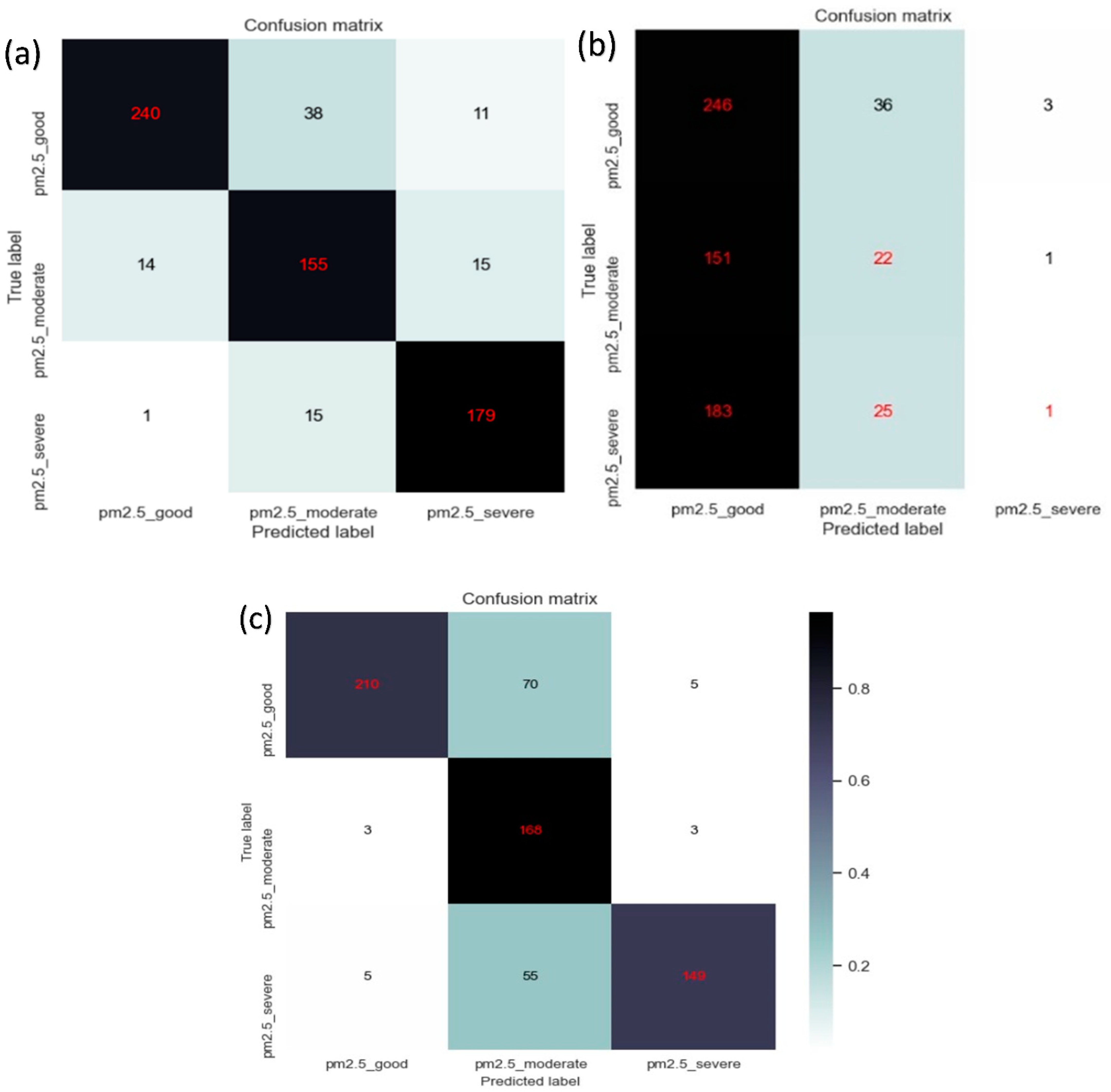
3. Results and Discussion
4. Conclusions
Supplementary Materials
Author Contributions
Funding
Institutional Review Board Statement
Informed Consent Statement
Data Availability Statement
Conflicts of Interest
References
- Kampa, M.; Castanas, E. Human health effects of air pollution. Environ. Pollut. 2008, 151, 362–367. [Google Scholar] [CrossRef]
- Lee, K.K.; Bing, R.; Kiang, J.; Bashir, S.; Spath, N.; Stelzle, D.; Mortimer, K.; Bularga, A.; Doudesis, D.; Joshi, S.S. Adverse health effects associated with household air pollution: A systematic review, meta-analysis, and burden estimation study. Lancet Glob. Health 2020, 8, e1427–e1434. [Google Scholar] [CrossRef]
- Liu, W.; Xu, Z.; Yang, T. Health effects of air pollution in China. Int. J. Environ. Res. Public Health 2018, 15, 1471. [Google Scholar] [CrossRef]
- Schraufnagel, D.E.; Balmes, J.R.; Cowl, C.T.; De Matteis, S.; Jung, S.-H.; Mortimer, K.; Perez-Padilla, R.; Rice, M.B.; Riojas-Rodriguez, H.; Sood, A. Air pollution and noncommunicable diseases: A review by the Forum of International Respiratory Societies’ Environmental Committee, Part 2: Air pollution and organ systems. Chest 2019, 155, 417–426. [Google Scholar] [CrossRef]
- Lelieveld, J.; Klingmüller, K.; Pozzer, A.; Pöschl, U.; Fnais, M.; Daiber, A.; Münzel, T. Cardiovascular disease burden from ambient air pollution in Europe reassessed using novel hazard ratio functions. Eur. Heart J. 2019, 40, 1590–1596. [Google Scholar] [CrossRef]
- Liu, C.; Chen, R.; Sera, F.; Vicedo-Cabrera, A.M.; Guo, Y.; Tong, S.; Coelho, M.S.; Saldiva, P.H.; Lavigne, E.; Matus, P. Ambient particulate air pollution and daily mortality in 652 cities. N. Engl. J. Med. 2019, 381, 705–715. [Google Scholar] [CrossRef]
- Miller, M.R. Oxidative stress and the cardiovascular effects of air pollution. Free Radic. Biol. Med. 2020, 151, 69–87. [Google Scholar] [CrossRef]
- Wang, N.; Mengersen, K.; Tong, S.; Kimlin, M.; Zhou, M.; Wang, L.; Yin, P.; Xu, Z.; Cheng, J.; Zhang, Y. Short-term association between ambient air pollution and lung cancer mortality. Environ. Res. 2019, 179, 108748. [Google Scholar] [CrossRef]
- Pang, Y.; Huang, W.; Luo, X.-S.; Chen, Q.; Zhao, Z.; Tang, M.; Hong, Y.; Chen, J.; Li, H. In-vitro human lung cell injuries induced by urban PM2. 5 during a severe air pollution episode: Variations associated with particle components. Ecotoxicol. Environ. Saf. 2020, 206, 111406. [Google Scholar] [CrossRef]
- Herget, W.F.; Brasher, J.D. Remote Fourier transform infrared air pollution studies. Opt. Eng. 1980, 19, 508–514. [Google Scholar] [CrossRef]
- Gosz, J.R.; Dahm, C.N.; Risser, P.G. Long-path FTIR measurement of atmospheric trace gas concentrations. Ecology 1988, 69, 1326–1330. [Google Scholar] [CrossRef]
- Russwurm, G.M.; Kagann, R.H.; Simpson, O.A.; McClenny, W.A.; Herget, W.F. Long-path FTIR measurements of volatile organic compounds in an industrial setting. J. Air Waste Manag. Assoc. 1991, 41, 1062–1066. [Google Scholar] [CrossRef]
- Bacsik, Z.; Komlósi, V.; Ollár, T.; Mink, J. Comparison of open path and extractive long-path ftir techniques in detection of air pollutants. Appl. Spectrosc. Rev. 2006, 41, 77–97. [Google Scholar] [CrossRef]
- Briz, S.; de Castro, A.J.; Díez, S.; López, F.; Schäfer, K. Remote sensing by open-path FTIR spectroscopy. Comparison of different analysis techniques applied to ozone and carbon monoxide detection. J. Quant. Spectrosc. Radiat. Transf. 2007, 103, 314–330. [Google Scholar] [CrossRef]
- Chang, P.-E.P.; Yang, J.-C.R.; Den, W.; Wu, C.-F. Characterizing and locating air pollution sources in a complex industrial district using optical remote sensing technology and multivariate statistical modeling. Environ. Sci. Pollut. Res. 2014, 21, 10852–10866. [Google Scholar] [CrossRef]
- Chen, C.-W.; Tseng, Y.-S.; Mukundan, A.; Wang, H.-C. Air Pollution: Sensitive Detection of PM2.5 and PM10 Concentration Using Hyperspectral Imaging. Appl. Sci. 2021, 11, 4543. [Google Scholar] [CrossRef]
- Ebner, A.; Zimmerleiter, R.; Cobet, C.; Hingerl, K.; Brandstetter, M.; Kilgus, J. Sub-second quantum cascade laser based infrared spectroscopic ellipsometry. Opt. Lett. 2019, 44, 3426–3429. [Google Scholar] [CrossRef]
- Yin, X.; Wu, H.; Dong, L.; Li, B.; Ma, W.; Zhang, L.; Yin, W.; Xiao, L.; Jia, S.; Tittel, F.K. ppb-Level SO2 Photoacoustic Sensors with a Suppressed Absorption–Desorption Effect by Using a 7.41 μm External-Cavity Quantum Cascade Laser. ACS Sens. 2020, 5, 549–556. [Google Scholar] [CrossRef]
- Zheng, F.; Qiu, X.; Shao, L.; Feng, S.; Cheng, T.; He, X.; He, Q.; Li, C.; Kan, R.; Fittschen, C. Measurement of nitric oxide from cigarette burning using TDLAS based on quantum cascade laser. Opt. Laser Technol. 2020, 124, 105963. [Google Scholar] [CrossRef]
- Ma, P.; Tao, F.; Gao, L.; Leng, S.; Yang, K.; Zhou, T. Retrieval of Fine-Grained PM2.5 Spatiotemporal Resolution Based on Multiple Machine Learning Models. Remote Sens. 2022, 14, 599. [Google Scholar] [CrossRef]
- Zhang, L.; Na, J.; Zhu, J.; Shi, Z.; Zou, C.; Yang, L. Spatiotemporal causal convolutional network for forecasting hourly PM2.5 concentrations in Beijing, China. Comput. Geosci. 2021, 155, 104869. [Google Scholar] [CrossRef]
- Liu, C.; Xing, C.; Hu, Q.; Wang, S.; Zhao, S.; Gao, M. Stereoscopic hyperspectral remote sensing of the atmospheric environment: Innovation and prospects. Earth-Sci. Rev. 2022, 226, 103958. [Google Scholar] [CrossRef]
- Meléndez, J.; Guarnizo, G. Fast quantification of air pollutants by mid-infrared hyperspectral imaging and principal component analysis. Sensors 2021, 21, 2092. [Google Scholar] [CrossRef] [PubMed]
- Liu, C.; Hu, Q.; Zhang, C.; Xia, C.; Yin, H.; Su, W.; Wang, X.; Xu, Y.; Zhang, Z. First Chinese ultraviolet–visible hyperspectral satellite instrument implicating global air quality during the COVID-19 pandemic in early 2020. Light Sci. Appl. 2022, 11, 28. [Google Scholar] [CrossRef] [PubMed]
- Nicks, D.; Baker, B.; Lasnik, J.; Delker, T.; Howell, J.; Chance, K.; Liu, X.; Flittner, D.; Kim, J. Hyperspectral remote sensing of air pollution from geosynchronous orbit with GEMS and TEMPO. In Proceedings of the Earth Observing Missions and Sensors: Development, Implementation, and Characterization V, Honolulu, HI, USA, 25–26 September 2018; pp. 118–124. [Google Scholar]
- Liu, C.; Xing, C.; Hu, Q.; Li, Q.; Liu, H.; Hong, Q.; Tan, W.; Ji, X.; Lin, H.; Lu, C. Ground-based hyperspectral stereoscopic remote sensing network: A promising strategy to learn coordinated control of O3 and PM2.5 over China. Engineering 2021, 7, 1–11. [Google Scholar] [CrossRef]
- Tsai, C.-L.; Mukundan, A.; Chung, C.-S.; Chen, Y.-H.; Wang, Y.-K.; Chen, T.-H.; Tseng, Y.-S.; Huang, C.-W.; Wu, I.-C.; Wang, H.-C. Hyperspectral Imaging Combined with Artificial Intelligence in the Early Detection of Esophageal Cancer. Cancers 2021, 13, 4593. [Google Scholar] [CrossRef]
- Chan, K.L.; Wang, Z.; Heue, K.-P. Hyperspectral ground based and satellite measurements of tropospheric NO2 and HCHO over Eastern China. In Proceedings of the Optical Sensors and Sensing Congress (ES, FTS, HISE, Sensors), San Jose, CA, USA, 25 June 2019; p. HTh1B.3. [Google Scholar]
- Jeon, E.-I.; Park, J.-W.; Lim, S.-H.; Kim, D.-W.; Yu, J.-J.; Son, S.-W.; Jeon, H.-J.; Yoon, J.-H. Study on the Concentration Estimation Equation of Nitrogen Dioxide using Hyperspectral Sensor. J. Korea Acad.-Ind. Coop. Soc. 2019, 20, 19–25. [Google Scholar]
- Schneider, A.; Feussner, H. Biomedical Engineering in Gastrointestinal Surgery; Academic Press: Cambridge, MA, USA, 2017. [Google Scholar]
- Lu, B.; Dao, P.D.; Liu, J.; He, Y.; Shang, J. Recent advances of hyperspectral imaging technology and applications in agriculture. Remote Sens. 2020, 12, 2659. [Google Scholar] [CrossRef]
- Mukundan, A.; Patel, A.; Saraswat, K.D.; Tomar, A.; Kuhn, T. Kalam Rover. In Proceedings of the AIAA SCITECH 2022 Forum, San Diego, CA, USA, 3–7 January 2022; p. 1047. [Google Scholar]
- Gross, W.; Queck, F.; Vögtli, M.; Schreiner, S.; Kuester, J.; Böhler, J.; Mispelhorn, J.; Kneubühler, M.; Middelmann, W. A multi-temporal hyperspectral target detection experiment: Evaluation of military setups. In Proceedings of the Target and Background Signatures VII, Online, 13–17 September 2021; pp. 38–48. [Google Scholar]
- Mukundan, A.; Feng, S.-W.; Weng, Y.-H.; Tsao, Y.-M.; Artemkina, S.B.; Fedorov, V.E.; Lin, Y.-S.; Huang, Y.-C.; Wang, H.-C. Optical and Material Characteristics of MoS2/Cu2O Sensor for Detection of Lung Cancer Cell Types in Hydroplegia. Int. J. Mol. Sci. 2022, 23, 4745. [Google Scholar] [CrossRef]
- Hsiao, Y.-P.; Mukundan, A.; Chen, W.-C.; Wu, M.-T.; Hsieh, S.-C.; Wang, H.-C. Design of a Lab-On-Chip for Cancer Cell Detection through Impedance and Photoelectrochemical Response Analysis. Biosensors 2022, 12, 405. [Google Scholar] [CrossRef]
- Mukundan, A.; Tsao, Y.-M.; Artemkina, S.B.; Fedorov, V.E.; Wang, H.-C. Growth Mechanism of Periodic-Structured MoS2 by Transmission Electron Microscopy. Nanomaterials 2021, 12, 135. [Google Scholar] [CrossRef] [PubMed]
- Gerhards, M.; Schlerf, M.; Mallick, K.; Udelhoven, T. Challenges and future perspectives of multi-/Hyperspectral thermal infrared remote sensing for crop water-stress detection: A review. Remote Sens. 2019, 11, 1240. [Google Scholar] [CrossRef]
- Lee, C.-H.; Mukundan, A.; Chang, S.-C.; Wang, Y.-L.; Lu, S.-H.; Huang, Y.-C.; Wang, H.-C. Comparative Analysis of Stress and Deformation between One-Fenced and Three-Fenced Dental Implants Using Finite Element Analysis. J. Clin. Med. 2021, 10, 3986. [Google Scholar] [CrossRef] [PubMed]
- Stuart, M.B.; McGonigle, A.J.; Willmott, J.R. Hyperspectral imaging in environmental monitoring: A review of recent developments and technological advances in compact field deployable systems. Sensors 2019, 19, 3071. [Google Scholar] [CrossRef] [PubMed]
- Mukundan, A.; Wang, H.-C. Simplified Approach to Detect Satellite Maneuvers Using TLE Data and Simplified Perturbation Model Utilizing Orbital Element Variation. Appl. Sci. 2021, 11, 10181. [Google Scholar] [CrossRef]
- Fang, Y.-J.; Mukundan, A.; Tsao, Y.-M.; Huang, C.-W.; Wang, H.-C. Identification of Early Esophageal Cancer by Semantic Segmentation. J. Pers. Med. 2022, 12, 1204. [Google Scholar] [CrossRef]
- Vangi, E.; D’Amico, G.; Francini, S.; Giannetti, F.; Lasserre, B.; Marchetti, M.; Chirici, G. The new hyperspectral satellite PRISMA: Imagery for forest types discrimination. Sensors 2021, 21, 1182. [Google Scholar] [CrossRef]
- Zhang, X.; Han, L.; Dong, Y.; Shi, Y.; Huang, W.; Han, L.; González-Moreno, P.; Ma, H.; Ye, H.; Sobeih, T. A deep learning-based approach for automated yellow rust disease detection from high-resolution hyperspectral UAV images. Remote Sens. 2019, 11, 1554. [Google Scholar] [CrossRef]
- Hennessy, A.; Clarke, K.; Lewis, M. Hyperspectral classification of plants: A review of waveband selection generalisability. Remote Sens. 2020, 12, 113. [Google Scholar] [CrossRef]
- Terentev, A.; Dolzhenko, V.; Fedotov, A.; Eremenko, D. Current State of Hyperspectral Remote Sensing for Early Plant Disease Detection: A Review. Sensors 2022, 22, 757. [Google Scholar] [CrossRef]
- De La Rosa, R.; Tolosana-Delgado, R.; Kirsch, M.; Gloaguen, R. Automated Multi-Scale and Multivariate Geological Logging from Drill-Core Hyperspectral Data. Remote Sens. 2022, 14, 2676. [Google Scholar] [CrossRef]

| RGB | Precision | Recall | F1 Score |
| Good | 96.33% | 73.68% | 83.50% |
| Moderate | 57.34% | 96.55% | 71.95% |
| Severe | 94.90% | 71.29% | 81.42% |
| PCA | Precision | Recall | F1 Score |
| Good | 94.12% | 83.04% | 88.24% |
| Moderate | 74.52% | 84.24% | 79.08% |
| Severe | 87.32% | 91.79% | 89.50% |
| 3D-CAE | Precision | Recall | F1 Score |
| Good | 42.41% | 86.32% | 56.88% |
| Moderate | 26.54% | 12.64% | 17.12% |
| Severe | 20.00% | 0.48% | 0.93% |
| Method | Classification Accuracy (%) |
|---|---|
| PCA | 85.93 |
| RGB | 78.89 |
| 3D-CAE | 40.27 |
Publisher’s Note: MDPI stays neutral with regard to jurisdictional claims in published maps and institutional affiliations. |
© 2022 by the authors. Licensee MDPI, Basel, Switzerland. This article is an open access article distributed under the terms and conditions of the Creative Commons Attribution (CC BY) license (https://creativecommons.org/licenses/by/4.0/).
Share and Cite
Mukundan, A.; Huang, C.-C.; Men, T.-C.; Lin, F.-C.; Wang, H.-C. Air Pollution Detection Using a Novel Snap-Shot Hyperspectral Imaging Technique. Sensors 2022, 22, 6231. https://doi.org/10.3390/s22166231
Mukundan A, Huang C-C, Men T-C, Lin F-C, Wang H-C. Air Pollution Detection Using a Novel Snap-Shot Hyperspectral Imaging Technique. Sensors. 2022; 22(16):6231. https://doi.org/10.3390/s22166231
Chicago/Turabian StyleMukundan, Arvind, Chia-Cheng Huang, Ting-Chun Men, Fen-Chi Lin, and Hsiang-Chen Wang. 2022. "Air Pollution Detection Using a Novel Snap-Shot Hyperspectral Imaging Technique" Sensors 22, no. 16: 6231. https://doi.org/10.3390/s22166231
APA StyleMukundan, A., Huang, C.-C., Men, T.-C., Lin, F.-C., & Wang, H.-C. (2022). Air Pollution Detection Using a Novel Snap-Shot Hyperspectral Imaging Technique. Sensors, 22(16), 6231. https://doi.org/10.3390/s22166231