Author Contributions
Conceptualization, D.T., S.Y. and K.W.; methodology, D.T., S.Y.; software, D.T.; validation, D.T., S.Y. and K.W.; formal analysis, D.T., S.Y. and K.W.; investigation, D.T., S.Y. and K.W.; resources, D.T., S.Y. and K.W.; data curation, D.T., S.Y. and K.W.; writing—original draft preparation, D.T., S.Y.; writing—review and editing, D.T., S.Y. and K.W.; visualization, D.T., S.Y.; supervision, S.Y. and K.W.; project administration, S.Y.; funding acquisition, S.Y. All authors have read and agreed to the published version of the manuscript.
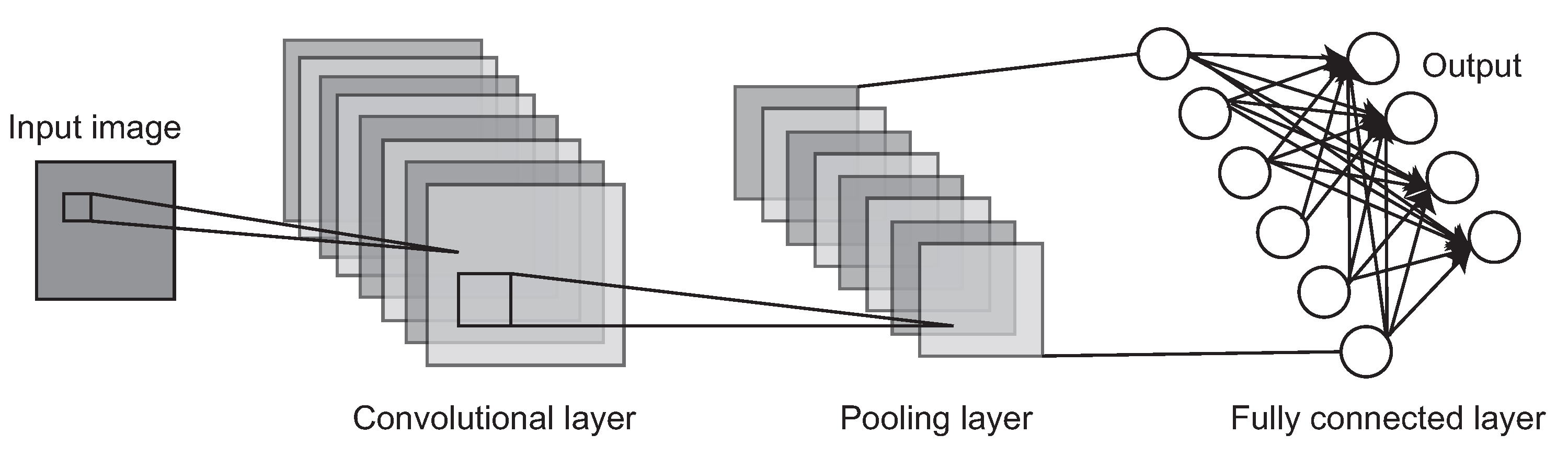
Figure 1.
A basic architecture of the Convolutional Neural Network (CNN). A typical CNN is mainly composed of a convolutional layer, a pooling layer and a fully connected layer.
Figure 1.
A basic architecture of the Convolutional Neural Network (CNN). A typical CNN is mainly composed of a convolutional layer, a pooling layer and a fully connected layer.
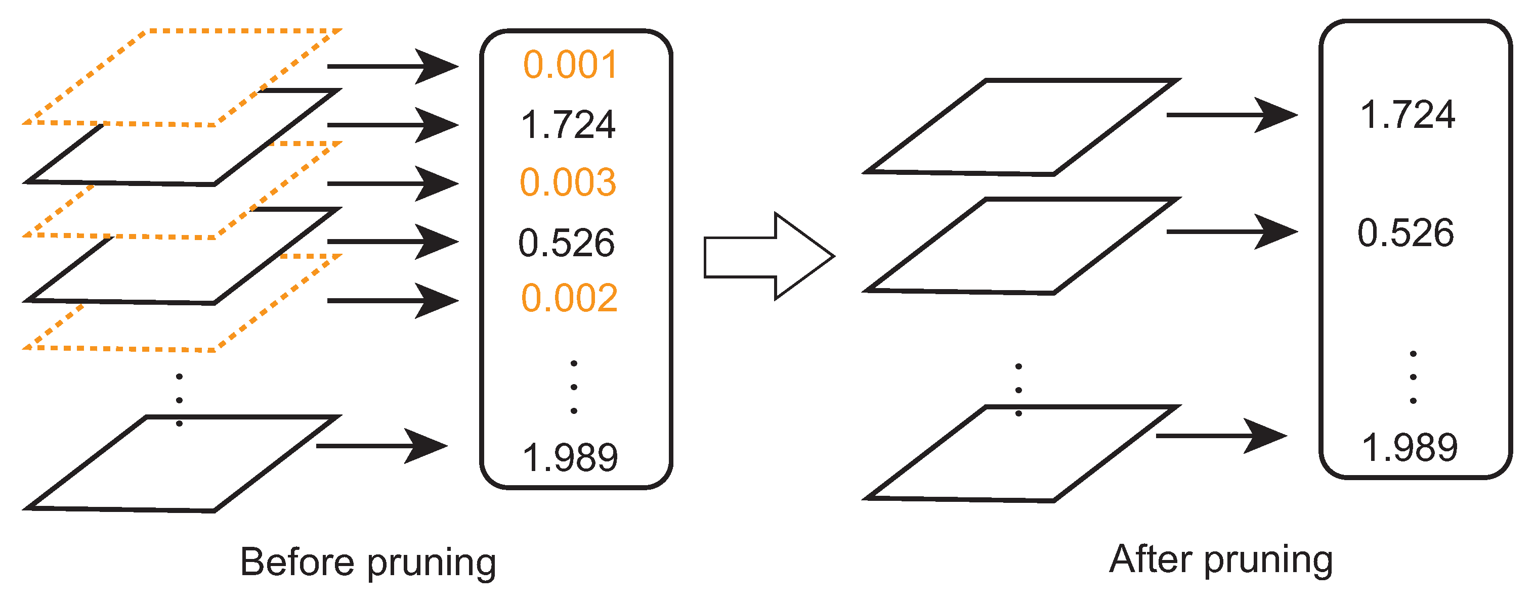
Figure 2.
The network slimming process. The channels (left side in orange color) with small scaling factor values (the numbers in orange color) will be eliminated.
Figure 2.
The network slimming process. The channels (left side in orange color) with small scaling factor values (the numbers in orange color) will be eliminated.
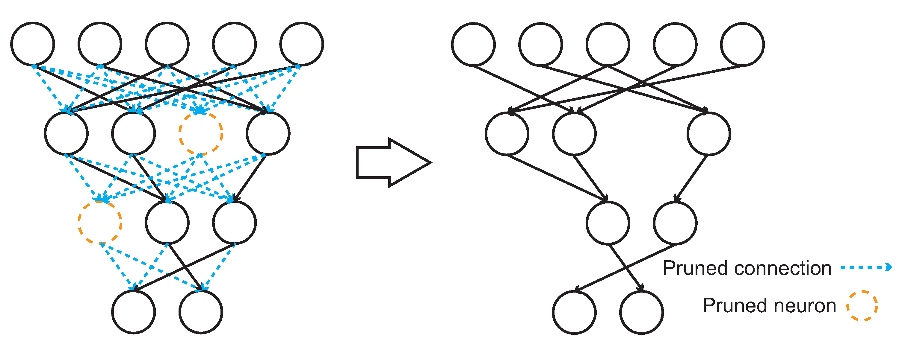
Figure 3.
The weight pruning process. The connections (left side in blue color) among neurons with small weight values will be eliminated. The neurons (left side in orange color) without any input or output connection will also be eliminated.
Figure 3.
The weight pruning process. The connections (left side in blue color) among neurons with small weight values will be eliminated. The neurons (left side in orange color) without any input or output connection will also be eliminated.
Figure 4.
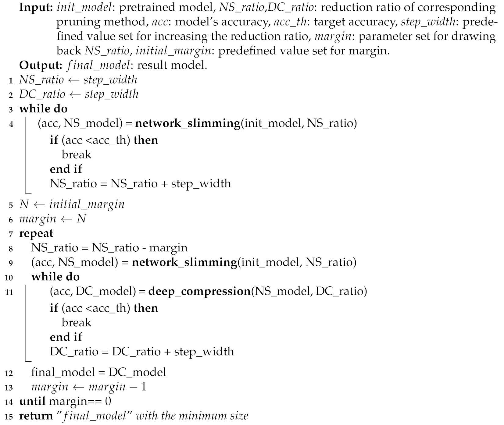
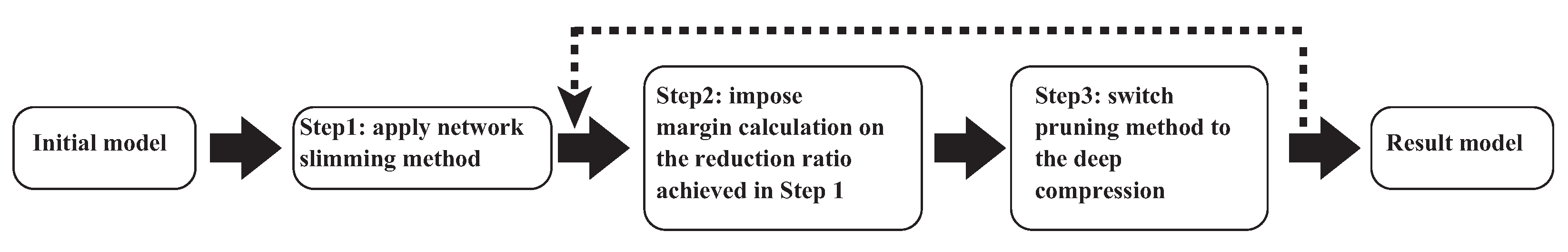
A flow chart of the three-step procedure of our proposed method.
Figure 4.
A flow chart of the three-step procedure of our proposed method.
Figure 5.
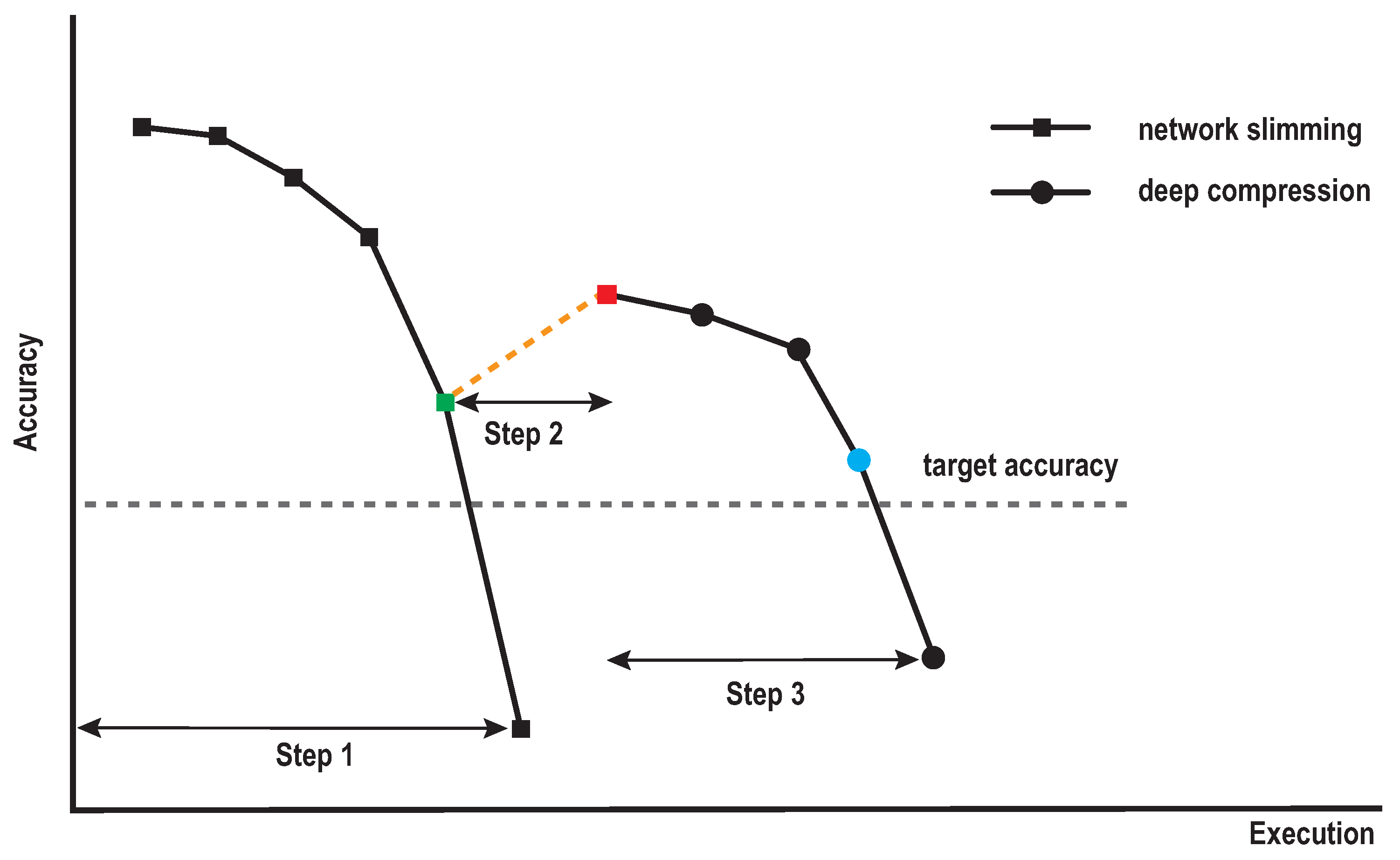
Compression iterations of our proposed method during the search process for the minimal accuracy. Step 1 is the iteration to find the minimal model by structured pruning. Step 2 is the iteration defined by the margin. Step 3 is the iteration to find the minimal model by the unstructured pruning.
Figure 5.
Compression iterations of our proposed method during the search process for the minimal accuracy. Step 1 is the iteration to find the minimal model by structured pruning. Step 2 is the iteration defined by the margin. Step 3 is the iteration to find the minimal model by the unstructured pruning.
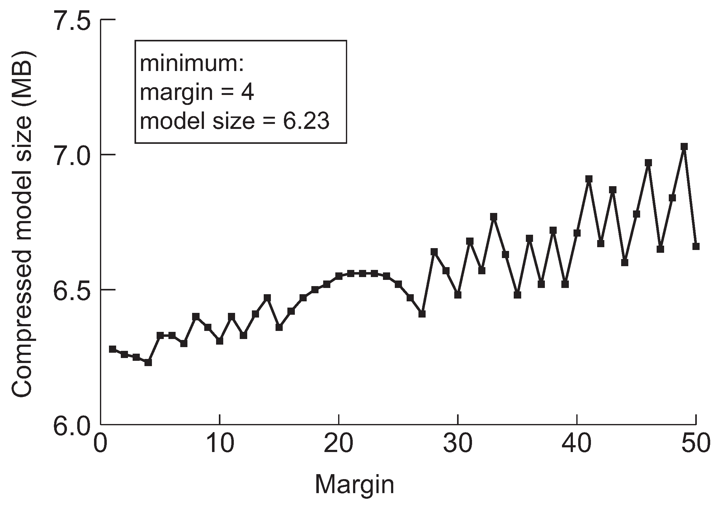
Figure 6.
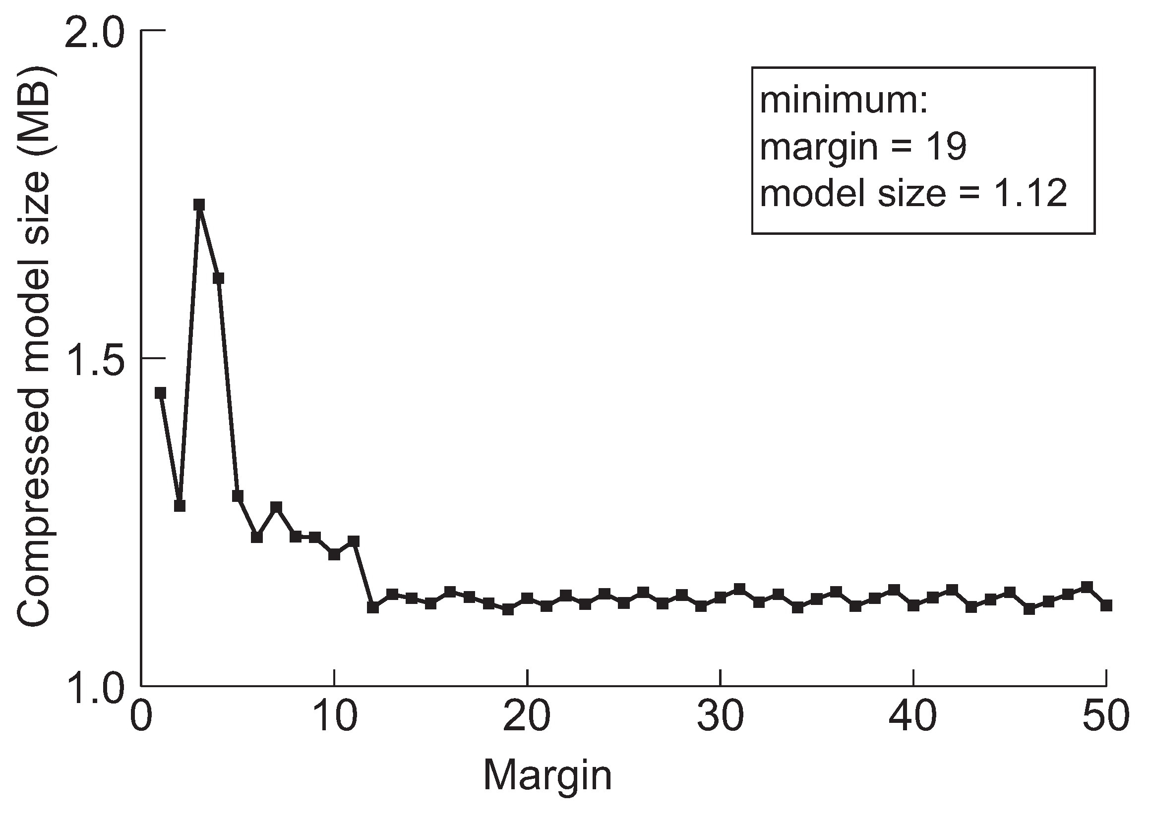
The minimum model sizes derived by the proposed method when the initial margin is varied from 1 to 50 for VGG-19 when the target accuracy is 92%.
Figure 6.
The minimum model sizes derived by the proposed method when the initial margin is varied from 1 to 50 for VGG-19 when the target accuracy is 92%.
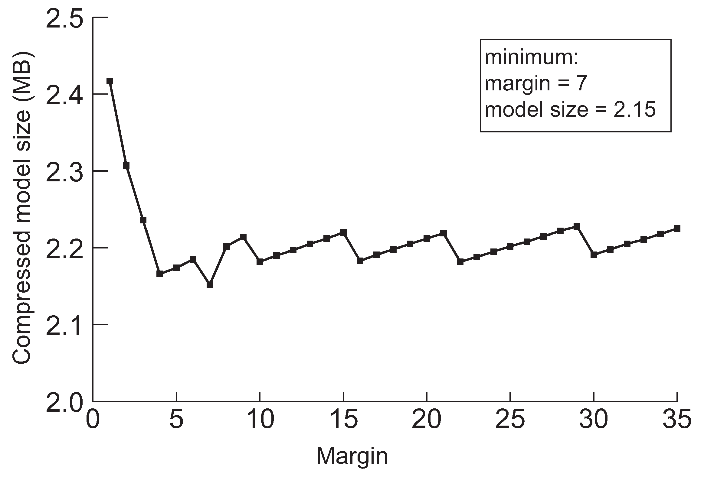
Figure 7.
The minimum model sizes derived by the proposed method when the initial margin is varied from 1 to 50 for ResNet-110 when the target accuracy is 94%.
Figure 7.
The minimum model sizes derived by the proposed method when the initial margin is varied from 1 to 50 for ResNet-110 when the target accuracy is 94%.
Figure 8.
The minimum model sizes derived by the proposed method when the initial margin is varied from 1 to 50 for DenseNet-40 when the target accuracy is 92%.
Figure 8.
The minimum model sizes derived by the proposed method when the initial margin is varied from 1 to 50 for DenseNet-40 when the target accuracy is 92%.
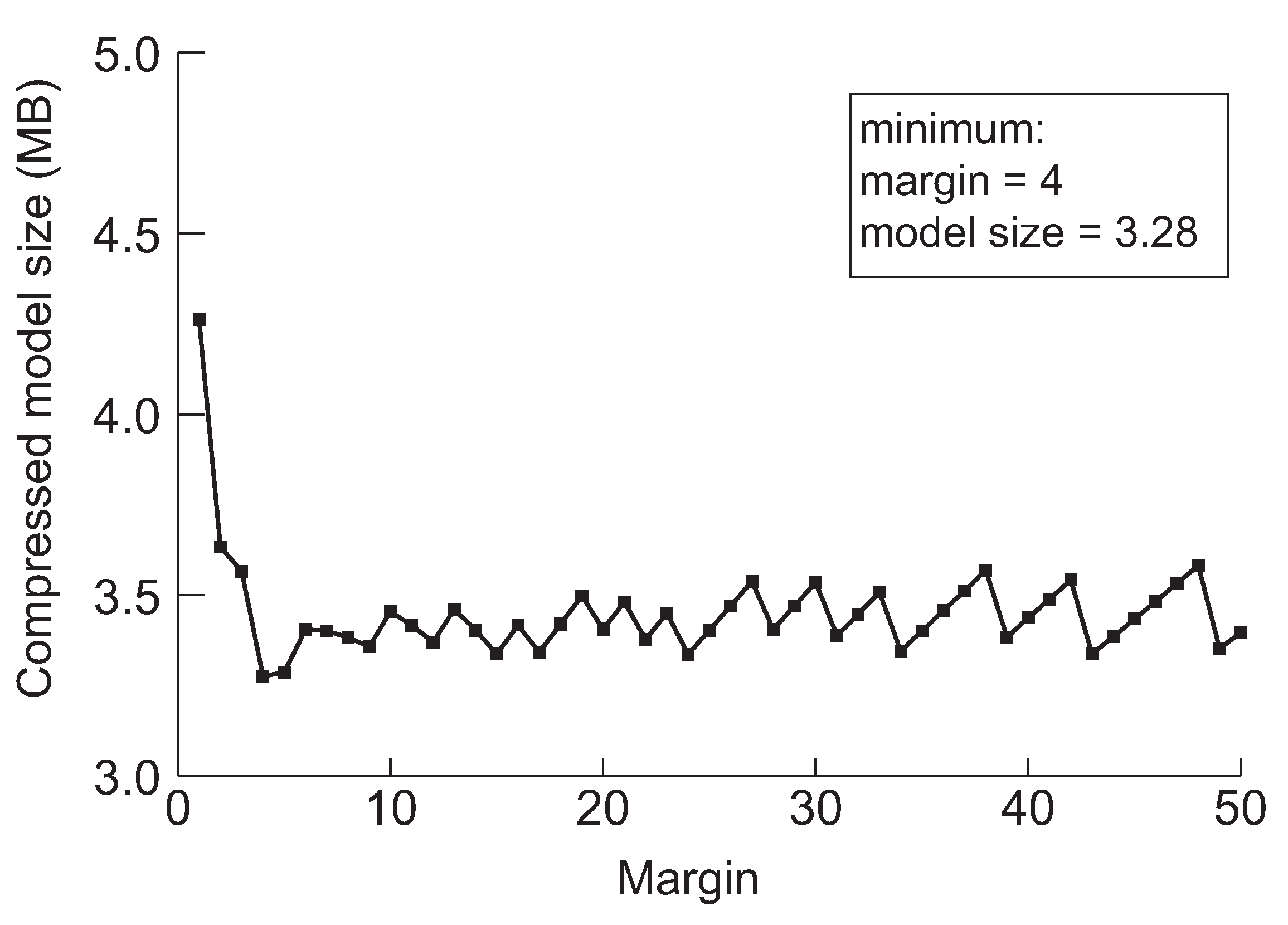
Figure 9.
The minimum model sizes derived by the proposed method when the initial margin is varied from 1 to 50 for DenseNet-121 when the target accuracy is 94%.
Figure 9.
The minimum model sizes derived by the proposed method when the initial margin is varied from 1 to 50 for DenseNet-121 when the target accuracy is 94%.
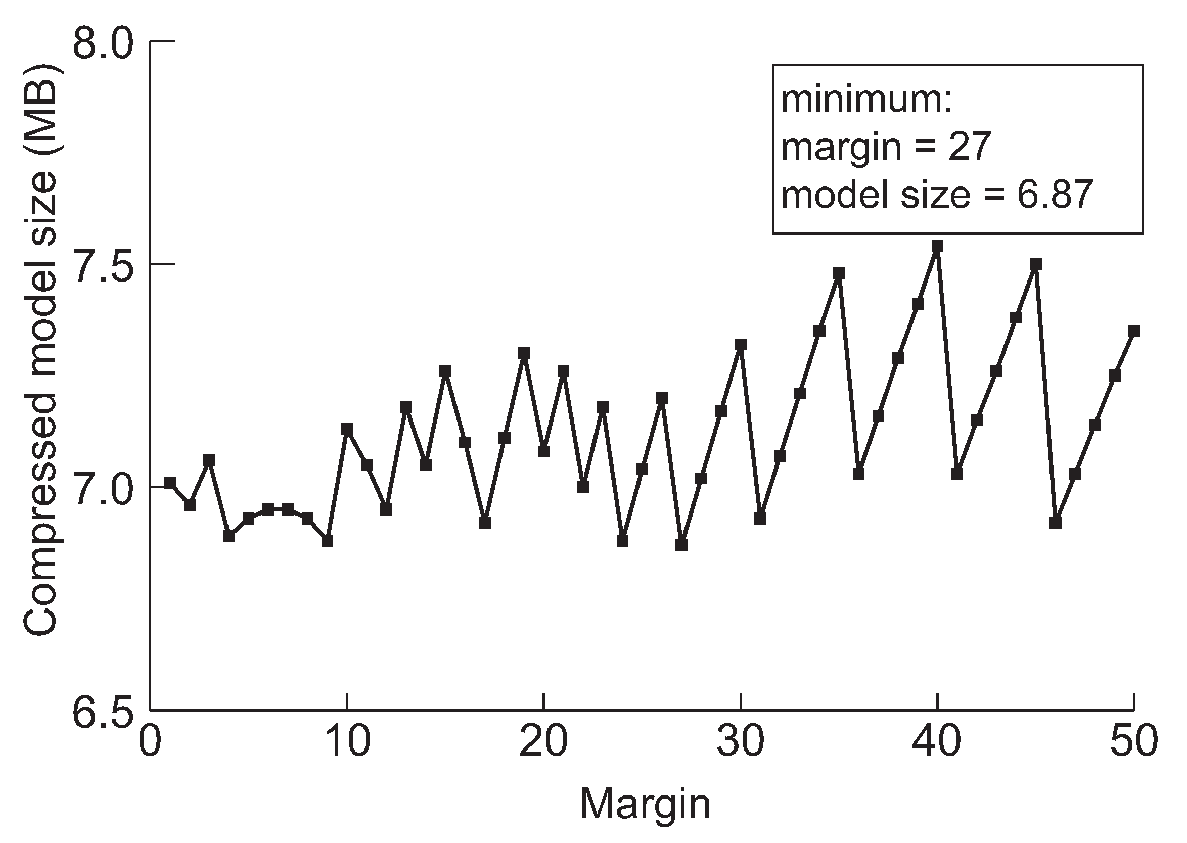
Figure 10.
The minimum model sizes derived by the proposed method when the initial margin is varied from 1 to 50 for DenseNet-202 when the target accuracy is 95%.
Figure 10.
The minimum model sizes derived by the proposed method when the initial margin is varied from 1 to 50 for DenseNet-202 when the target accuracy is 95%.
Table 1.
The original model size and accuracies of CNN models used in experiments.
Table 1.
The original model size and accuracies of CNN models used in experiments.
| Model | Accuracy | Model Size |
|---|
| VGG-19 | 93.99% | 80.34 MB |
| ResNet-110 | 94.59% | 4.61 MB |
| DenseNet-40 | 94.16% | 4.26 MB |
| DenseNet-121 | 95.51% | 42.15 MB |
| DenseNet-202 | 95.99% | 117.24 MB |
Table 2.
The sizes of the minimized models in the corresponding accuracies derived from the proposed method and the individual cases of network slimming and deep compression for VGG-19.
Table 2.
The sizes of the minimized models in the corresponding accuracies derived from the proposed method and the individual cases of network slimming and deep compression for VGG-19.
| Target Accuracy | Deep Compression | Network Slimming | Ours (Margin) |
|---|
| 85% | 6.42 MB | 10.2 MB | 5.91 MB (4) |
| 90% | 7.23 MB | 10.2 MB | 6.11 MB (5) |
| 92% | 7.23 MB | 10.2 MB | 6.23 MB (4) |
Table 3.
The sizes of the minimized models in the corresponding accuracies derived from the proposed method and the individual cases of network slimming and deep compression for ResNet-110.
Table 3.
The sizes of the minimized models in the corresponding accuracies derived from the proposed method and the individual cases of network slimming and deep compression for ResNet-110.
| Target Accuracy | Deep Compression | Network Slimming | Ours (Margin) |
|---|
| 85% | 1.14 MB | 3.77 MB | 1.13 MB (20) |
| 90% | 1.46 MB | 3.87 MB | 1.44 MB (40) |
| 94% | 2.19 MB | 4.06 MB | 2.15 MB (7) |
Table 4.
The sizes of the minimized models in the corresponding accuracies derived from the proposed method and the individual cases of network slimming and deep compression for DenseNet-40.
Table 4.
The sizes of the minimized models in the corresponding accuracies derived from the proposed method and the individual cases of network slimming and deep compression for DenseNet-40.
| Target Accuracy | Deep Compression | Network Slimming | Ours (Margin) |
|---|
| 85% | 0.71 MB | 1.81 MB | 0.68 MB (21) |
| 90% | 0.92 MB | 1.97 MB | 0.90 MB (16) |
| 92% | 1.13 MB | 2.02 MB | 1.12 MB (19) |
Table 5.
The sizes of the minimized models in the corresponding accuracies derived from the proposed method and the individual cases of network slimming and deep compression for DenseNet-121.
Table 5.
The sizes of the minimized models in the corresponding accuracies derived from the proposed method and the individual cases of network slimming and deep compression for DenseNet-121.
| Target Accuracy | Deep Compression | Network Slimming | Ours (Margin) |
|---|
| 85% | 2.49 MB | 8.30 MB | 2.28 MB (22) |
| 90% | 2.90 MB | 8.72 MB | 2.49 MB (25) |
| 94% | 3.73 MB | 9.96 MB | 3.73 MB (4) |
Table 6.
The sizes of the minimized models in the corresponding accuracies derived from the proposed method and the individual cases of network slimming and deep compression for DenseNet-202.
Table 6.
The sizes of the minimized models in the corresponding accuracies derived from the proposed method and the individual cases of network slimming and deep compression for DenseNet-202.
| Target Accuracy | Deep Compression | Network Slimming | Ours (Margin) |
|---|
| 85% | 4.69 MB | 15.10 MB | 3.52 MB (50) |
| 90% | 4.69 MB | 15.10 MB | 4.32 MB (29) |
| 95% | 7.03 MB | 19.07 MB | 6.87 MB (27) |
Table 7.
The execution times in the corresponding accuracies derived from the proposed method and the individual cases of network slimming and deep compression for VGG-19.
Table 7.
The execution times in the corresponding accuracies derived from the proposed method and the individual cases of network slimming and deep compression for VGG-19.
| Target Accuracy | Brute-Force Search Method | Ours (Number of Accuracy Check) |
|---|
| 85% | 7.5 h | 0.5 h (656) |
| 90% | 7.5 h | 0.5 h (659) |
| 92% | 7.5 h | 0.5 h (654) |
Table 8.
The execution times in the corresponding accuracies derived from the proposed method and the individual cases of network slimming and deep compression for ResNet-110.
Table 8.
The execution times in the corresponding accuracies derived from the proposed method and the individual cases of network slimming and deep compression for ResNet-110.
| Target Accuracy | Brute-Force Search Method | Ours (Number of Accuracy Check) |
|---|
| 85% | 8.3 h | 0.45 h (597) |
| 90% | 8.3 h | 0.35 h (470) |
| 94% | 8.3 h | 0.30 h (388) |
Table 9.
The execution times in the corresponding accuracies derived from the proposed method and the individual cases of network slimming and deep compression for DenseNet-40.
Table 9.
The execution times in the corresponding accuracies derived from the proposed method and the individual cases of network slimming and deep compression for DenseNet-40.
| Target Accuracy | Brute-Force Search Method | Ours (Number of Accuracy Check) |
|---|
| 85% | 7.5 h | 0.6 h (663) |
| 90% | 7.5 h | 0.6 h (678) |
| 92% | 7.5 h | 0.5 h (579) |
Table 10.
The execution times in the corresponding accuracies derived from the proposed method and the individual cases of network slimming and deep compression for DenseNet-121.
Table 10.
The execution times in the corresponding accuracies derived from the proposed method and the individual cases of network slimming and deep compression for DenseNet-121.
| Target Accuracy | Brute-Force Search Method | Ours (Number of Accuracy Check) |
|---|
| 85% | 28 h | 2.1 h (737) |
| 90% | 28 h | 1.9 h (690) |
| 94% | 28 h | 2.0 h (705) |
Table 11.
The execution times in the corresponding accuracies derived from the proposed method and the individual cases of network slimming and deep compression for DenseNet 202.
Table 11.
The execution times in the corresponding accuracies derived from the proposed method and the individual cases of network slimming and deep compression for DenseNet 202.
| Target Accuracy | Brute-Force Search Method | Ours (Number of Accuracy Check) |
|---|
| 85% | 92.5 h | 6.3 h (689) |
| 90% | 92.5 h | 6.35 h (719) |
| 95% | 92.5 h | 6.5 h (739) |
Table 12.
The sizes of the minimized models in the corresponding accuracies derived from the individual cases of network slimming and deep compression, NS→DC and DC→NS for VGG-19.
Table 12.
The sizes of the minimized models in the corresponding accuracies derived from the individual cases of network slimming and deep compression, NS→DC and DC→NS for VGG-19.
| Target Accuracy | Deep Compression | Network Slimming | NS→DC | DC→NS |
|---|
| 85% | 6.42 MB | 10.2 MB | 5.91 MB | 7.23 MB |
| 90% | 7.23 MB | 10.2 MB | 6.11 MB | 8.03 MB |
| 92% | 7.23 MB | 10.2 MB | 6.23 MB | 8.03 MB |
Table 13.
The sizes of the minimized models in the corresponding accuracies derived from the individual cases of network slimming and deep compression, NS→DC and DC→NS for ResNet-110.
Table 13.
The sizes of the minimized models in the corresponding accuracies derived from the individual cases of network slimming and deep compression, NS→DC and DC→NS for ResNet-110.
| Target Accuracy | Deep Compression | Network Slimming | NS→DC | DC→NS |
|---|
| 85% | 1.14 MB | 3.77 MB | 1.13 MB | 1.17 MB |
| 90% | 1.46 MB | 3.87 MB | 1.44 MB | 1.47 MB |
| 94% | 2.19 MB | 4.06 MB | 2.15 MB | 2.19 MB |
Table 14.
The sizes of the minimized models in the corresponding accuracies derived from the individual cases of network slimming and deep compression, NS→DC and DC→NS for DenseNet-40.
Table 14.
The sizes of the minimized models in the corresponding accuracies derived from the individual cases of network slimming and deep compression, NS→DC and DC→NS for DenseNet-40.
| Target Accuracy | Deep Compression | Network Slimming | NS→DC | DC→NS |
|---|
| 85% | 0.71 MB | 1.81 MB | 0.68 MB | 0.73 MB |
| 90% | 0.92 MB | 1.97 MB | 0.90 MB | 0.94 MB |
| 92% | 1.13 MB | 2.02 MB | 1.12 MB | 1.14 MB |
Table 15.
The sizes of the minimized models in the corresponding accuracies derived from the individual cases of network slimming and deep compression, NS→DC and DC→NS for DenseNet-121.
Table 15.
The sizes of the minimized models in the corresponding accuracies derived from the individual cases of network slimming and deep compression, NS→DC and DC→NS for DenseNet-121.
| Target Accuracy | Deep Compression | Network Slimming | NS→DC | DC→NS |
|---|
| 85% | 2.49 MB | 8.30 MB | 2.28 MB | 2.55 MB |
| 90% | 2.90 MB | 8.72 MB | 2.49 MB | 2.96 MB |
| 94% | 3.73 MB | 9.96 MB | 3.28 MB | 3.89 MB |
Table 16.
The sizes of the minimized models in the corresponding accuracies derived from the individual cases of network slimming and deep compression, NS→DC and DC→NS for DenseNet-202.
Table 16.
The sizes of the minimized models in the corresponding accuracies derived from the individual cases of network slimming and deep compression, NS→DC and DC→NS for DenseNet-202.
| Target Accuracy | Deep Compression | Network Slimming | NS→DC | DC→NS |
|---|
| 85% | 4.69 MB | 15.09 MB | 3.52 MB | 4.84 MB |
| 90% | 4.69 MB | 15.09 MB | 4.32 MB | 5.15 MB |
| 95% | 7.03 MB | 19.07 MB | 6.87 MB | 8.21 MB |


