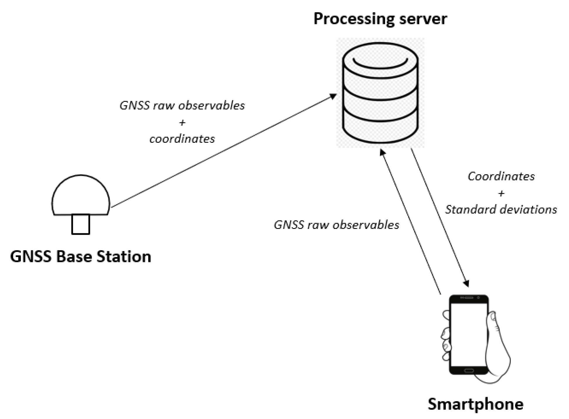
In this section, the effects on GNSS positioning by smartphones introduced by the application of the MDP algorithm are discussed. In particular, the performance of the algorithm, in terms of multipath detection and mitigation, under varying configuration parameters is detailed. For this purpose, both static and kinematic data sets are analysed. The selected case studies are used to test the main features of the proposed architecture. They are both processed using the LIGE base station, developed for this work. They require the use of our Android app installed on a device and the modified RTKLIB version for data processing. Although the proposed architecture has been designed for real-time applications, in order to evaluate the performance of the MDP algorithm, several post-processing elaborations were computed, all having the same input data and therefore being under the same contextual conditions.
The values to be associated with the various parameters to achieve optimal results may depend on various factors (e.g., environmental conditions and hardware characteristics of the receiver) and are still an object of research. For the two case studies, some PPK processing was performed considering different combinations of the parameters, as explained later. Concerning the rest of the processing options used in RTKLIB for PPK positioning, the ionosphere and troposhere models used are the Klobuchar and Saastamoinen, respectively. Only the broadcast ephemeris were considered, and an elevation mask of 15° is also set. The solution type selected is “forward” for both case studies.
5.1. Static Test
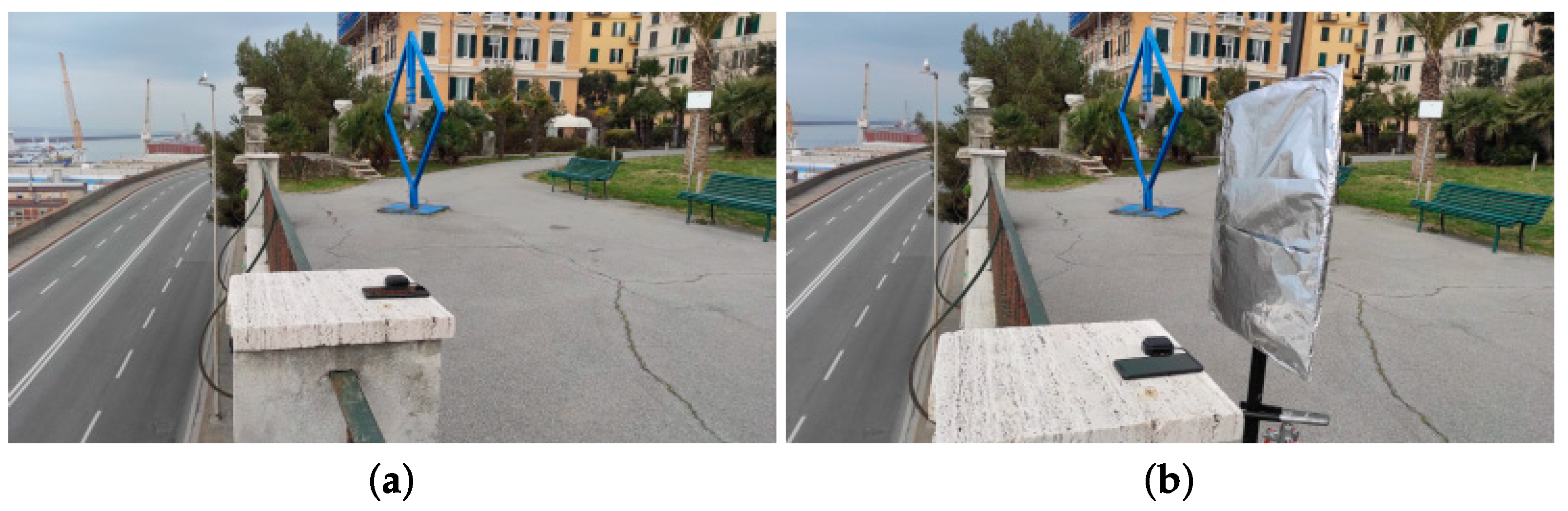
The static data set refers to the acquisition described in
Section 2. The MDP trend is presented for both the receivers used, with the purpose of understanding the MDP performance in detecting multipath errors for smartphone receivers with respect to a classic GNSS receiver.
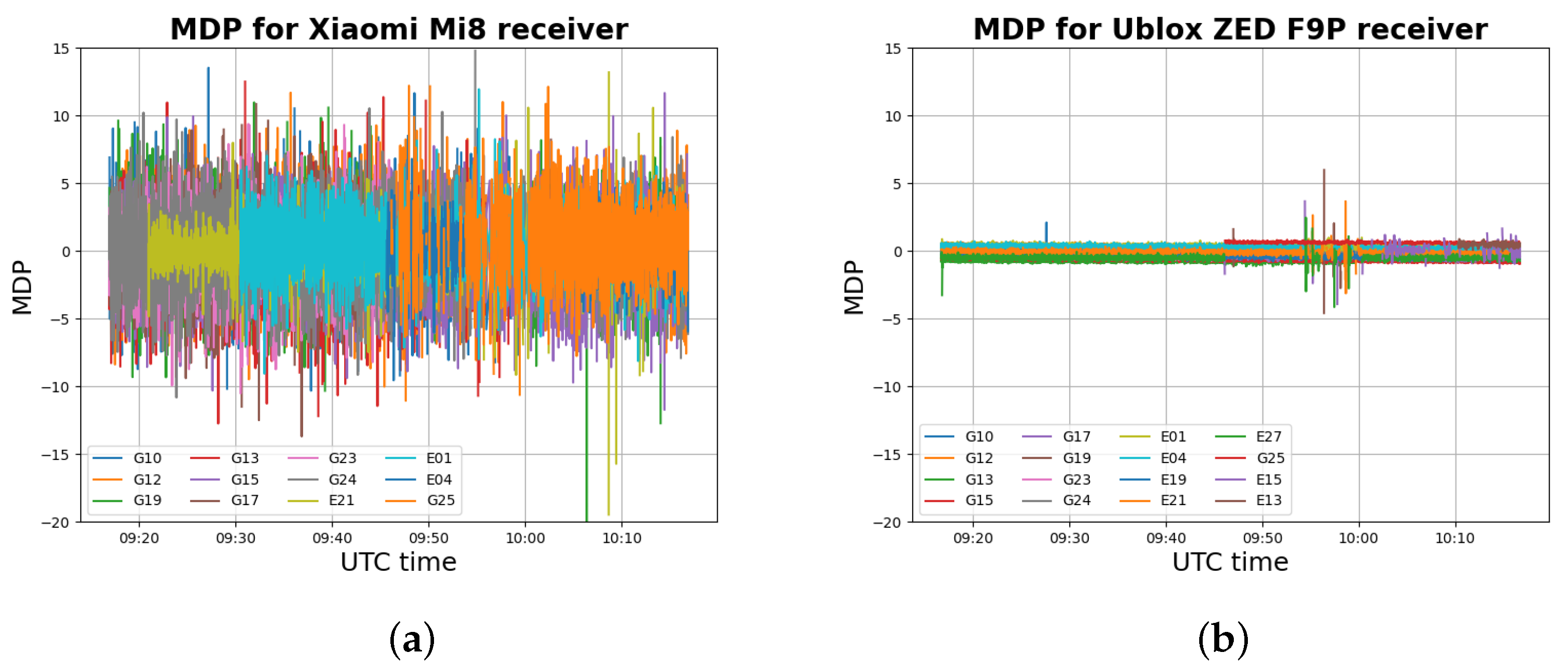
Figure 9 shows the MDP values detected by the Xiaomi Mi8 and the u-blox ZED F9P.
The MDP variable is representative of the multipath effect and residual errors due to external noise (see Equation (
5)).
Figure 9 shows that the MDP variable for the u-blox ZED F9P receiver has some peaks between the 9:45 and 10:00 UTC, that is, when the multipath effect was induced, as discussed in
Section 2. The MDP variable can then be considered a reasonable multipath indicator for this kind of receiver. For the Xiaomi Mi8 receiver, the MDP variable presents a noisy trend with higher values in modulus. Differently from the u-blox ZED F9P, the Xiaomi Mi8 MDP trend has more diffuse peaks and is not particularly concentrated between 9:45 and 10:00 UTC. Nevertheless, a couple of peaks can be noted for the Xiaomi Mi8 in that interval. The noisier trend of the Xiaomi Mi8 MDP variable with respect to the u-blox ZED F9P can be explained by higher values of the external noise caused by the poor quality of the smartphone’s antenna. This makes the MDP variable less effective in multipath identification for smartphones receivers.
For evaluating the performance of the MDP algorithm for the smartphone receiver, processing was computed under changing configuration parameters. Data were processed using all three criteria proposed for multipath detection. For every criterion, both static and adaptive MDP thresholds were used, as specified below.
Concerning the static threshold, six values were selected on the basis of the MDP trend (
Figure 9a). The chosen values of the MDP static threshold are 2.5, 3.0, 3.5, 4.0, 4.5, and 5 m. These values have been selected after several tests, as discussed in [
27], and indications from the literature.
For the adaptive threshold, six different windows (number of epochs) are selected: 10, 20, 30, 40, 50, and 60. The window size times the acquisition rate determines an initialisation time in which the algorithm cannot be applied. Considering that all smartphones have an acquisition rate of 1 Hz, an initialisation time no longer than 1 min (i.e., 60 epochs) was considered in the experiments.
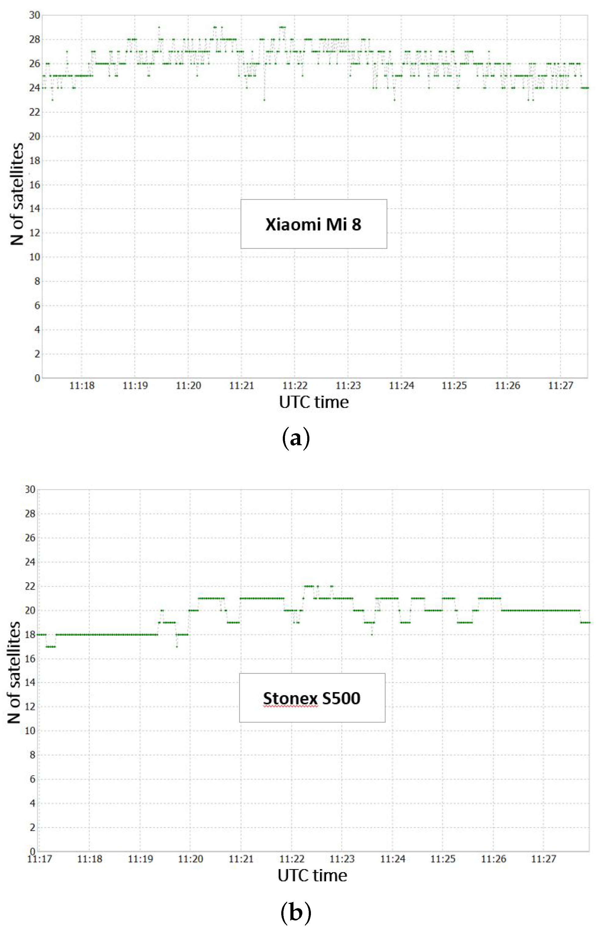
Finally, considering the SNR trend for the Xiaomi Mi8 receiver (
Figure 6a), four values of the SNR threshold are considered: 20, 25, 30, and 35 DB-Hz. Again, these values have been selected after several tests, as discussed in [
27], and indications from the literature.
Combining all these option values, we considered 108 different experimental tests. Hereafter, the most interesting results are reported. The interested reader may refer to Lorenzo Benvenuto’s PhD thesis for a complete description of the experiments [
27].
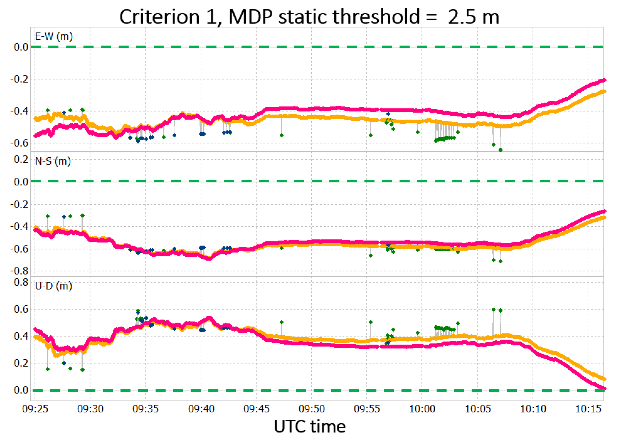
Considering criterion 1, the solutions obtained for the static MDP threshold values, compared with the solution without the MDP algorithm application, are shown in
Figure 10.
In
Figure 10, the solutions obtained after the MDP algorithm is applied are depicted in pink and blue for float and fixed solutions, respectively, while the solution obtained without the application of MDP algorithm is depicted in yellow and green for float and fixed solutions, respectively. In the figure, the precise coordinates of the point are also highlighted with the dashed green line. The data set presents a convergence time of about 5 min, which is not considered for the results analysis.
The solution, after the application of the MDP algorithm, has slight improvements in terms of accuracy, especially in the case of MDP threshold equal to 2.5. Considering the planimetric accuracy, an improvement of 5 cm is obtained. Over all the threshold values considered for this criterion, this is the best result reached. The worst result obtained is the one with an MDP threshold value of 5.0 m (see [
27]).
As additional experiment, the data set has been processed considering the adaptive MDP threshold with a time window containing 30 epochs. This window size has been selected after additional experiments (from 10 to 60 epochs) discussed in [
27]. The positioning results concerning the processing executed with criterion 1 and the adaptive MDP threshold compared with the solution without the MDP algorithm application are reported in
Figure 11.
The solution obtained with the application of the MDP algorithm is in pink and blue, and the solution obtained without its application is in yellow and green; the precise coordinates of the point are represented by the dashed green line. In this case, improvements are present in the solution accuracy not only with respect to the case without the MDP algorithm application, but also with respect to the case with the static MDP threshold equal to 2.5 m. The difference in terms of RMS for the three cases is reported in
Table 3.
The results shown in
Table 3 can be explained by the fact that the adaptive threshold is more selective than the static threshold in the identification of data potentially affected by multipath. When dealing with very noisy GNSS observables, such as those produced by smartphones, the usage of a static MDP threshold may lead to consideration of any data that are not affected by multipath as outliers in the MDP trend. Reducing the weights of those data still leads to some benefits in terms of positioning accuracy, but those benefits are lower with respect to the ones obtained if only multipath-affected observables (i.e., outliers in the MDP trend) will be assigned a reduced weight. Concerning the precision of the solutions, appreciable differences are noted in the STD of the solutions, so it can be stated that the MDP algorithm does not lead to improvement in positioning precision.
From
Figure 10 and
Figure 11, it can be seen that the best improvements are obtained during the period of the induced multipath (i.e., from 9:45 to 10:00 UTC). The solution obtained for both adaptive and static threshold in that time interval are depicted in
Figure 12. For the rest of the period, the solutions with and without the application of the MDP algorithm are quite similar.
In
Figure 12, the solution obtained with the MDP algorithm presents an unstable set of fixed solutions. However, fixed solutions obtained without the MDP algorithm often turned out to be false solutions. Indeed, their RMS is in the order of tens of centimetres, while, for fixed solutions, the expected RMS should be in the order of few centimetres. In this sense, an unstable set of results that is still consistent with the rest of the obtained positions seems to be preferable to false fixed solutions. Therefore, the MDP heuristics seems to increase the robustness of the positioning process in the selected test battery.
The differences in terms of RMS for the adaptive threshold case and static one are reported in
Table 4.
Similarly to the whole test period, in this time interval, the solution accuracy particularly increases when the adaptive threshold is considered. Considering that the multipath error was manually induced in this time interval, the MDP algorithm seems to be effective in mitigating this type of error.
In criterion 2, the observable is considered to be affected by multipath if its SNR value is lower than its threshold, and at the same time, the MDP value in modulus is higher than the current MDP threshold. Considering the static MDP threshold, the major improvements are obtained for MDP threshold equal to 2.5 m, so the impact of the SNR value is discussed only for this situation. The statistics in terms of the RMS referred to in our experiments are reported in
Table 5.
In the case of the SNR threshold set to 20 DB-Hz, very low improvements can be noted in term of accuracy with respect to the solution without the MDP algorithm. This means that very few observations have the condition on MDP and SNR simultaneosly. Compared to the results in
Table 3, the introduction of a very low SNR threshold worsens the performance of the algorithm in improving the accuracy of the solution. In addition, no significant improvements in terms of solution robustness can be observed in this case. Considering the case with SNR threshold equal to 35 DB-Hz instead, some improvements in terms of accuracy can be observed. Furthermore, if an SNR threshold equal to 35 DB-Hz is considered, the number of false fixed solutions is reduced with respect to the “no MDP” case. This means that the solution robustness is increased.
Some additional tests for criterion 2 considered the adaptive MDP threshold. In these cases, no significant differences were obtained with respect to the results for criterion 1. Indeed, as previously noted, the MDP adaptive threshold, differently from the static one, only selects a few outliers in the MDP trend. The SNR threshold instead selects many pieces of data, especially if its value is set to 35 DB-Hz. Considering that for criterion 2, the MDP and SNR condition must be verified at the same time, it is reasonable to deduce that the discarded data in this case are the same as those selected via criterion 1 where the SNR is not checked for the detection part of the algorithm.
Summarizing, it is possible to state that, considering criterion 2, the usage of the SNR values for the detection phase of the MDP algorithm has advantages for the mitigation performance of the algorithm itself, if a static MDP threshold is considered. Those benefits regard the position accuracy and robustness, and they are more evident for increasing values for the SNR threshold. No differences are introduced by the usage of SNR in the detection part if the MDP adaptive threshold is selected. No appreciable differences can be observed, for all the processing executed for this criterion, in terms of STD.
5.2. Kinematic Test
The kinematic data set refers to the pedestrian acquisition described in
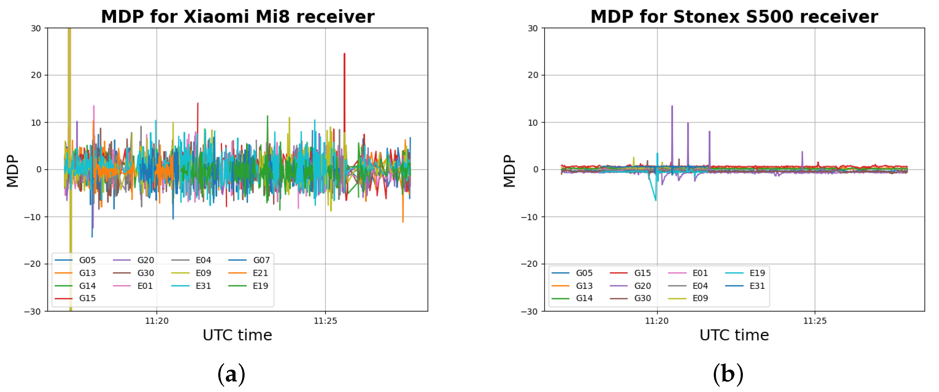
Section 2. As for the static case study, the MDP trend is presented for both receivers, with the purpose of understanding the MDP performance of detecting multipath for smartphone receivers compared to more traditional GNSS receivers.
Similarly to what observed for the static case study, the MDP variable for the smartphone receiver (
Figure 13a) is noisier compared to of a classic GNSS receiver. The chosen values for the MDP static threshold are: 2.5, 3.0, 3.5, 4.0, 4.5, and 5 m. For the adaptive threshold, considering the results obtained for the static case study, only 30 previous epochs were considered for the threshold computation. Finally, considering the SNR trend for the Xiaomi Mi8 receiver (
Figure 3a), four values of the SNR threshold were considered: 20, 25, 30, and 35 DB-Hz. Combining all these option values, 63 different processing results were obtained. Hereafter, the obtained results are reported.
The best results for criterion 1 were obtained considering the MDP threshold equal to 2.5 m. The RMS results for the static part are reported in
Table 6. In order to justify the better improvements obtained with the MDP threshold equal to 2.5 m with respect to the other tested values, the worst result obtained (i.e., MDP threshold equal to 5.0 m) is also reported in the table.
As shown in
Table 6, some improvements in terms of accuracy are obtained after the MDP algorithm application. The MDP algorithm seems particularly effective in improving the accuracy of the solution when the MDP threshold equal to 2.5 m is considered.
Concerning the kinematic part, the application of the MDP algorithm produces some local benefits in the solution with the elimination of some outliers observed in the “NO MDP” solution. This means that in those intervals, the robustness of the solution is increased. Nevertheless, the MDP algorithm seems to introduce some outliers that were not observed in the “NO MDP” solution due to the fact that some data not affected by multipath were under-weighted by the algorithm. Using the static MDP threshold for multipath identification seems to work well if the receiver is static, but it seems to be not so effective if the receiver is moving.
Criterion 1 coupled with the adaptive MDP threshold was also tested for this case study. Unlike the results obtained for the static MDP threshold, the solution accuracy in this case is degraded if the static part of the data set is considered, as shown in
Table 7.
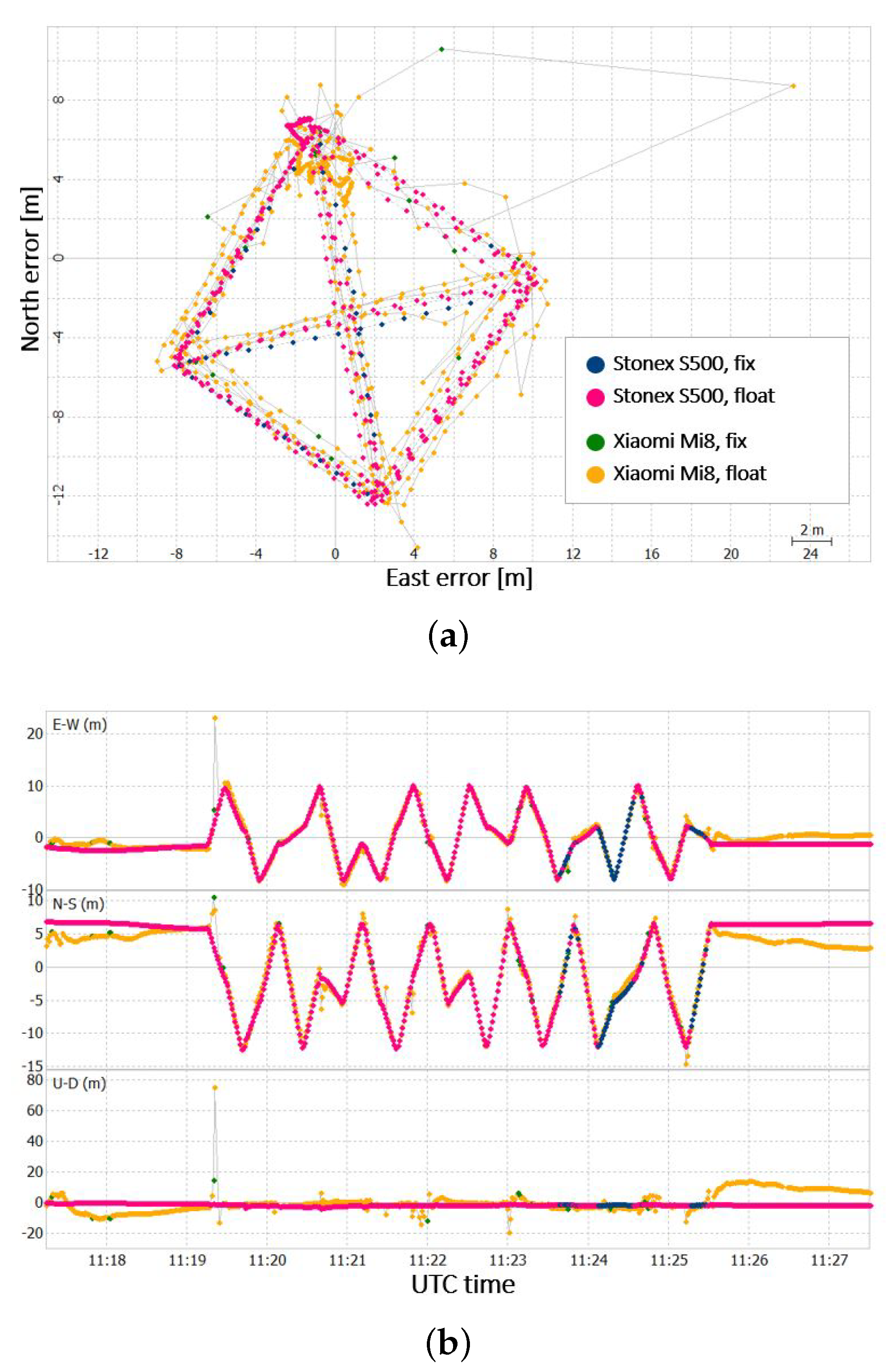
This result highlights that for this case study, the adaptive SNR threshold seems to be less effective in multipath recognition. Nevertheless, a significant improvement in the position accuracy can be noted for the East and North components after 11:18 UTC. After this instant, the planimetric accuracy is improved by about 11 cm, as the 2D RMS passes from 3.642 m to 3.528 m. This means that the bad performance of the MDP multipath detection is limited to the first few epochs of the data set.
Concerning the kinematic part of the data set, a similar behaviour to the one observed for the static MDP threshold is obtained. Nevertheless, in this case, some improvements are shown. The adaptive MDP threshold solution does not in fact have some of the outliers that the static MDP solution presents, especially for the Height component. This means that if the criterion 1 is considered for kinematic data sets, the usage of the adaptive MDP threshold seems preferable to the usage of a static MDP threshold [
27].
Hereafter, the results for criterion 2 are exposed with particular attention to the role played by the SNR threshold in the detection part of the MDP algorithm. Among all the MDP static threshold values considered, the best results were obtained for the threshold value equal to 2.5 m, which is consistent with the results observed for criterion 1. Varying the SNR threshold value, it was noted that the solution accuracy, at least for the static part, improves as the threshold value increases. Further processing was carried out by raising the SNR threshold value from 35 to 40 DB-Hz, but no significant differences were noted, as shown in
Table 8.
From the SNR value reported, we observe that the accuracy of the solution in this interval is improved by about 19 cm, 35 cm, and 52 cm for the East, North, and Height components, respectively. The planimetric accuracy of the solution is improved by 73 cm. It is also interesting to note the difference in RMS between this solution and the one obtained for criterion 1 (for comparison, see
Table 6), that is, without the usage of SNR for the multipath detection part. Concerning the kinematic part, no substantial differences are observed with respect to the criterion 1 case. It can be stated then that the solution obtained for criterion 2 is better in terms of accuracy compared to the one obtained for criterion 1, in the case of an MDP static threshold, especially for the static part of the test. Therefore, in static condition, considering both the SNR and MDP values for the detection part of the MDP algorithm increases the performance of the algorithm itself. The situation is different for the kinematic part, in which no differences are noted. In this case, it seems that using the SNR value does not provide any advantage to the detection part of the MDP algorithm.
The test with criterion 2 also involved the usage of the adaptive MDP threshold. In this cases, varying the SNR threshold value, no significant differences were reported with respect to the results already obtained for criterion 1, so the results are not shown. It can then be stated that for criterion 2, if the adaptive MDP threshold is considered, the usage of the SNR value does not improve the performance of the detection part of the MDP algorithm.
The kinematic part of this data set shows behaviour analogous to that obtained for the processing carried out for criteria 1 and 2. No further improvements are observed for this case study, and the same considerations, already discussed for the other cases, are valid also for this obtained result.


