An Efficient and Frequency-Scalable Algorithm for the Evaluation of Relative Permittivity Based on a Reference Data Set and a Microstrip Ring Resonator


Abstract
:1. Introduction
2. A Brief Reference to the Previous Procedure
3. The Proposed Algorithm Based on the Reference Data Set
3.1. The Approach to Creating a Reference Data Set
3.2. Data Fitting Algorithms
3.3. A Fitting Attempt with Exponential Functions
3.4. Polynomial Fitting Attempt
3.5. Shape-Preserving Algorithm for the “Horizontal” Data Fitting
3.6. The “Vertical” Interpolation of the Data (between the Reference Curves)
4. Benchmark Testing
5. Flexibility and Frequency Scalability of the Reference Data Set
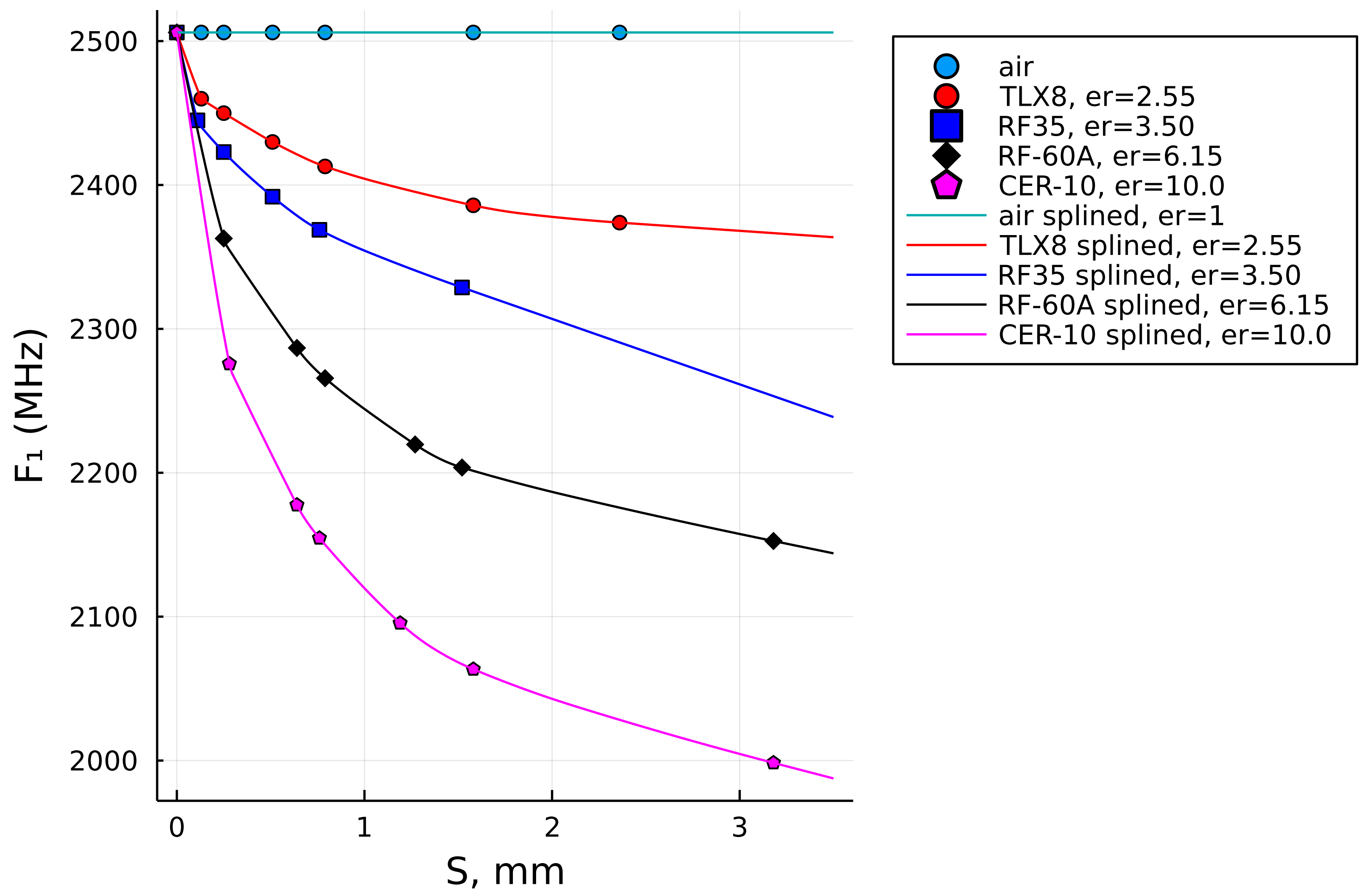
5.1. Extending the Reference Data for the Thicker Samples
5.2. Frequency Scaling of the Reference Data
6. Discussion on the Characteristics of This Approach
- Besides the measurements of and , which are necessary by either algorithm, the VMA requires multiple calculations of the integral (4). First, two capacitances, and , have to be computed to evaluate (1). Then, vector has to be computed to evaluate (3), for which the integral in (4) has to be run N times, where N is the length of vector . Although the overall procedure to determine the relative permittivity of some material is, by its nature, a fairly slow process, where a few more seconds do not make much difference, and modern personal computers can conduct the computational part of the process in about 20 s, give or take a few seconds, the VMA is numerically quite demanding, not to mention that in (1), one has to vary the dielectric materials when computing and , while in computing (3), has to be varied within the chosen arbitrary range, which makes the overall calculation subtle.Unlike that, RDSA avoids the computation of the challenging integral. The RDSA algorithm simply takes the given value of the SUT thickness S, measures , and scans through the well-interpolated reference data set, searching for the closest match between S (on the abscissa) and (on the ordinate). Due to that, the RDSA, with the initial reference data set, takes only about 1/10 of the computation time of the VMA, for the comparable accuracy within 10% of error with respect to the nominal value of the permittivity, based on multiple tests we conducted with the samples presented here. Even when the original reference set was extended, as discussed in Section 5.1, and the number of the interpolation points increased, in order to maintain a fair resolution of the SUT thickness points with the extended data set, the computation did not suffer any noticeable extra time and barely changed, for example, from 0.26 s for the initial data set to 0.43 s for the extended data set, which is a negligible difference for this purpose, by all means.
- Using a full-wave solver, the preparation of the reference data set was conducted in a consistent and unbiased way by means of 3D computational models, just as was the computation of the loaded resonant frequency for the reference thicknesses. Such a computational approach provides accuracy of the dimensions of the SUTs and their consistent placements on the surface of the MRR, just as it was intended, without introducing random errors from one sample to another.
- We believe that this algorithm can be used with some other dielectric-characterization methods or for characterization of magnetic materials, in which case each curve would just be represented by a different independent and dependent variable, while the principle of the algorithm would remain the same.
6.1. Means to Further Improve the Accuracy
- (a)
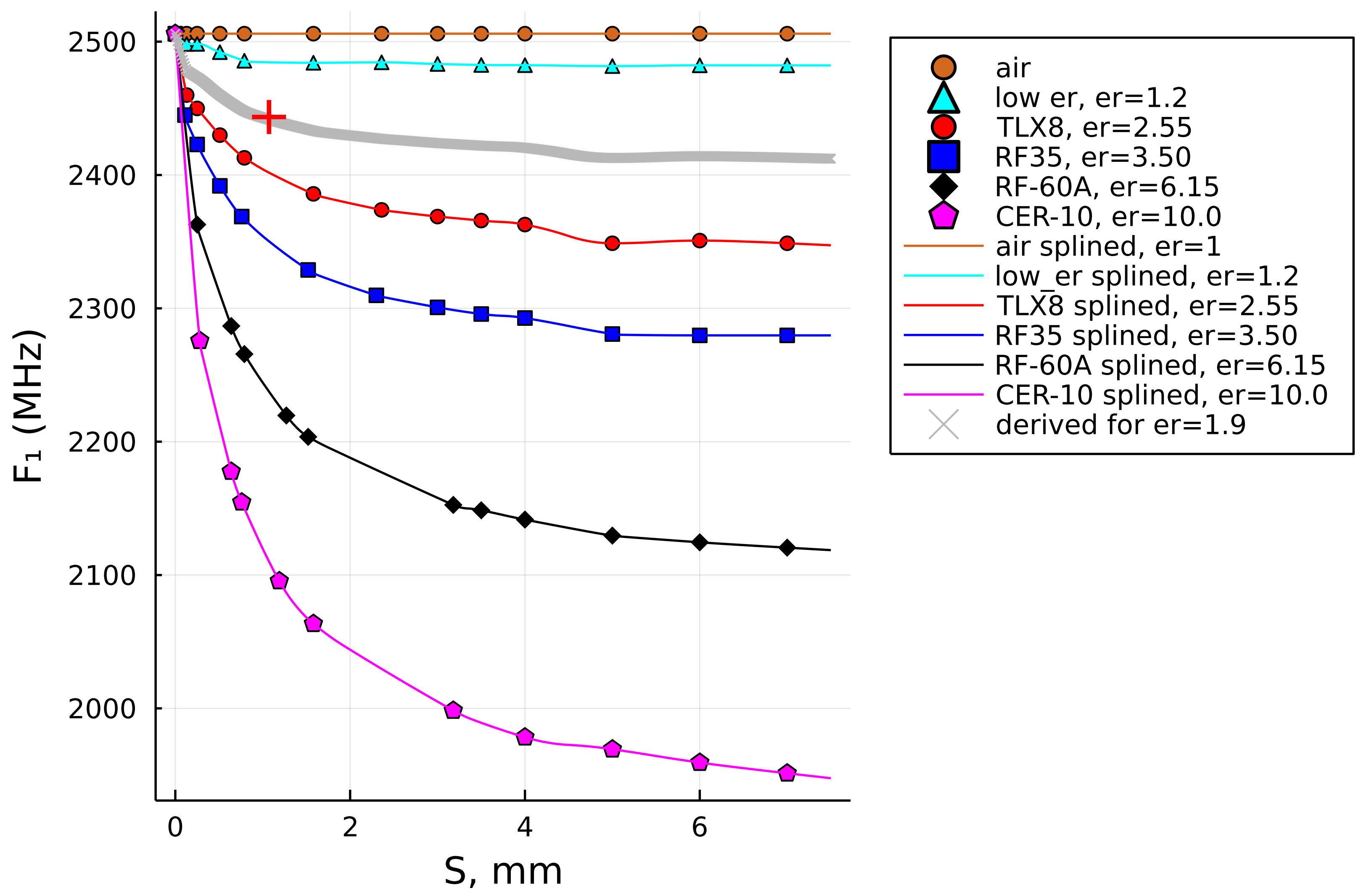
- Having more reference permittivity curves in order to lessen the vertical separation between the reference curves (in Section 3.6; we referred to it as the “vertical interpolation”).It is easy to prepare a new reference vector for any desired permittivity if the situation for any sample of interest would suggest that the space between any two adjacent curves be lessened for the sake of greater accuracy of the solution. An example is illustrated in Figure 10 where a curve with (the “low er” cyan curve) is inserted between the air curve and the TLX8 curve () to eventually improve the accuracy of the solution for the jeans sample, for example. Without this curve, the obtained solution by the RDSA was , while with this added curve, the newly obtained solution, shown by the red plus sign on the grey solution curve, is , which is closer to the quoted nominal value. The result could have possibly been even better if the “lower” curve had been prepared for , for example, thereby further reducing the space between it and the TLX8 curve.
- (b)
- Eventually having more data in the horizontal direction, i.e., having more sample thickness points for the reference data set. In this paper, this means having more reference resonant frequency values as a function of the sample thickness (see (11) and the discussion in Section 5.1). With a computational model, it is easy to add more reference points. However, with a small variance of the curve, its benefit is limited.
- (c)
- Setting a smaller step in the vertical interpolation stage of the algorithm (), but it has its limitations regarding the resulting improvement, depending on the actual quantity of the reference data. In other words, it is not a problem to reduce the step size, but it might not reach any better result for the particular case of interest. For example, when was reduced from 0.1 to 0.01, the final result on jeans permittivity slightly improved from 1.9 to 1.87, while for the glass sample, it improved from 6.85 to 6.80.
- (d)
- Eventually setting a smaller step size in the horizontal interpolation, to make sure the Schumaker-spline data fitting work as well as possible, but in our testing so far, the interpolation performs just as well with a smaller number of the interpolation points along the abscissa, as with an increased number of them. In this case, this was due to the monotonicity of these curves, while in the case of some other reference data set (i.e., by some other method), reducing might have a more significant impact.
6.2. A Comparison to Other Works
7. Conclusions
Supplementary Materials
Funding
Institutional Review Board Statement
Informed Consent Statement
Data Availability Statement
Acknowledgments
Conflicts of Interest
Abbreviations
| MRR | microstrip ring resonator |
| SUT | sample under test |
| PTFE | polytetrafluoroethylene |
| SPA | shape-preserving algorithm |
| VMA | variational method-based algorithm |
| RDSA | reference data set-based algorithm |
References
- Balanis, C.A. Antenna Theory: Analysis and Design, 3rd ed.; Wiley-Interscience: Hoboken, NJ, USA, 2005. [Google Scholar]
- Pozar, D.M. Microwave Engineering, 4th ed; J. Wiley and Sons: Hoboken, NJ, USA, 2011. [Google Scholar]
- Gupta, K.C.; Garg, R.; Bahl, I.; Bhartia, P. Microstrip Lines and Slotlines, 2nd ed.; Artech House: Norwood, MA, USA, 1996. [Google Scholar]
- Chen, L.F.; Ong, C.K.; Neo, C.P.; Varadan, V.V.; Varadan, V.K. Microwave Electronics: Measurement and Materials Characterization; John Wiley & Sons: Hoboken, NJ, USA, 2004. [Google Scholar]
- Taconic. Available online: https://www.agc-multimaterial.com/ (accessed on 10 November 2021).
- Rogers Corporation. Available online: https://rogerscorp.com/ (accessed on 10 November 2021).
- DuPont. Available online: https://www.dupont.com (accessed on 10 November 2021).
- FR-4 PCB Manufacturers. Available online: https://www.pcbdirectory.com/manufacturers?material=FR-4 (accessed on 10 November 2021).
- Martín, F.; Vélez, P.; Gil, M. Microwave Sensors Based on Resonant Elements. Sensors 2020, 20, 3375. [Google Scholar] [CrossRef]
- Phommakesone, S. DC-to-THz Electromagnetic Characterization of Materials. Webinar, 30 January 2022. Available online: https://connectlp.keysight.com/DC-to-THz-Electromagnetic-Characterization-28566 (accessed on 15 February 2022).
- Yap, D. Resonant Cavity Measurement Technique for Low-Loss Dielectric Materials. Webinar, 30 January 2022. Available online: https://connectlp.keysight.com/Resonant-Cavity-Measurement-32394 (accessed on 15 February 2022).
- Al-Mously, S.I.Y. A Modified Complex Permittivity Measurement Techniqueat Microwave Frequency. Int. J. New Comput. Archit. Their Appl. 2012, 2, 390–402. [Google Scholar]
- Venkatesh, M.; Raghavan, G. An overview of dielectric properties measuring techniques. Can. Biosyst. Eng. 2005, 47, 7.15–7.30. [Google Scholar]
- Baker-Jarvis, J.; Janezic, M.D.; John H. Grosvenor, J.; Geyer, R.G. Transmission/Reflection and Short-Circuit Line Methods for Measuring Permittivity Transmission/Reflection and Short-Circuit Line Methods for Measuring Permittivity and Permeability; NIST Tecnnical Note 1355-R; National Institute of Standards and Technology: Boulder, CO, USA, 1993. [Google Scholar]
- Janezic, M.D.; Williams, D.F. Permittivity Characterization from Transmission-line Measurement. In Proceedings of the 1997 IEEE MTT-S International Microwave Symposium Digest, Denver, CO, USA, 8–13 June 1997; IEEE MTT-S Digest. IEEE: Piscataway, NJ, USA, 1997. [Google Scholar]
- Janezic, M.D.; Jargon, J.A. Complex Permittivity Determination from Propagation Constant Measurements. IEEE Microw. Guid. Wave Lett. 1999, 9, 76–78. [Google Scholar] [CrossRef] [Green Version]
- Narayanan, P.M. Microstrip Transmission Line Method for Broadband Permittivity Measurement of Dielectric Substrates. IEEE Trans. Microw. Theory Tech. 2014, 62, 2784–2790. [Google Scholar] [CrossRef]
- Radonic, V.; Cselyuszka, N.; Crnojevic-Bengin, V.; Kitic, G. Phase-Shift Transmission Line Method for Permittivity Measurement and Its Potential in Sensor Applications. In Electromagnetic Materials and Devices [Internet]; Han, M., Ed.; InTech Open: London, UK, 2018; pp. 1–22. [Google Scholar]
- Sundaram, M. Transmission and Reflection Method With a Material Filled Transmission Line for Measuring Dielectric Properties. Master’s Thesis, University of Tennessee, Knoxville, TN, USA, 2004. [Google Scholar]
- Bogner, A.; Steiner, C.; Walter, S.; Kita, J.; Hagen, G.; Moos, R. Planar Microstrip Ring Resonators for Microwave-Based Gas Sensing: Design Aspects and Initial Transducers for Humidity and Ammonia Sensing. Sensors 2017, 17, 2422. [Google Scholar] [CrossRef]
- Heinola, J.M.; Lätti, K.P.; Ström, J.P.; Kettunen, M.; Silventoinen, P. Determination of dielectric constant and dissipation factor of a printed circuit board material using a microstrip ring resonator structure. In Proceedings of the 15th International Conference on Microwaves, Radar and Wireless Communications (IEEE Cat. No.04EX824), Warsaw, Poland, 17–19 May 2004; Volume 1, pp. 202–205. [Google Scholar] [CrossRef]
- Low, P.J.; Esa, F.; You, K.Y.; Abbas, Z. Estimation of Dielectric Constant for Various Standard Materials using Microstrip Ring Resonator. J. Sci. Technol. 2017, 9, 55–59. [Google Scholar]
- Waldron, I. Ring Resonator Method for Dielectric Permittivity Measurement of Foams. Master’s Thesis, Worcester Polytechnic Institute, Electrical and Computer Engineering, Worcester, MA, USA, 2006. [Google Scholar]
- Bernard, P.A.; Gautray, J.M. Measurement of Dielectric Constant Using a Microstrip Ring Resonator. IEEE Trans. Microw. Theory Tech. 1991, 39, 592–595. [Google Scholar] [CrossRef]
- Lee, C.S.; Yang, C.L. Complementary Split-Ring Resonators for Measuring Dielectric Constants and Loss Tangents. IEEE Microw. Wirel. Compon. Lett. 2014, 24, 563–565. [Google Scholar] [CrossRef]
- Grove, T.T.; Masters, M.F.; Miers, R.E. Determining dielectric constants using a parallel plate capacitor. Am. J. Phys. 2005, 73, 52–56. [Google Scholar] [CrossRef] [Green Version]
- Kumar, A.; Sharma, S. Measurement of Dielectric Constant and Loss Factor of the Dielectric Material at Microwave Frequencies. Prog. Electromagn. Res. 2007, 69, 47–54. [Google Scholar] [CrossRef] [Green Version]
- QWED. Split Post Dielectric Resonator. 2021. Available online: https://www.qwed.com.pl/resonators_spdr.html (accessed on 15 May 2022).
- Smith, D.R.; Vier, D.C.; Koschny, T.; Soukoulis, C.M. Electromagnetic parameter retrieval from inhomogeneous metamaterials. Phys. Rev. E 2005, 71, 036617. [Google Scholar] [CrossRef] [PubMed] [Green Version]
- Xu, Y.; Ghannouchi, F.M.; Bosisio, R. Theoretical and Experimental Study of Measurement of Microwave Permittivity Using Open Ended Elliptical Coaxial Probes. IEEE Trans. Microw. Theory Tech. 1992, 40, 143–150. [Google Scholar] [CrossRef]
- Keysight Technologies. N1501A Dielectric Probe Kit. 2020. Available online: https://www.keysight.com/zz/en/product/N1501A/dielectric-probe-kit.html (accessed on 8 July 2022).
- SPEAG. DAK. 2020. Available online: https://speag.swiss/products/dak/overview/ (accessed on 8 July 2022).
- Copper Mountain Technologies. Available online: https://coppermountaintech.com/ (accessed on 10 January 2022).
- Joler, M.; Raj, A.N.; Bartolić, J. A Simplified Measurement Configuration for Evaluation of Relative Permittivity Using a Microstrip Ring Resonator with a Variational Method-Based Algorithm. Sensors 2022, 22, 928. [Google Scholar] [CrossRef]
- Joler, M.; Raj, A.N.J.; Bartolić, J. Finding an Optimal Sample Size and Placement for Measurement of Relative Permittivity using a Microstrip Ring Resonator. In Proceedings of the 29th International Conference on Software, Telecommunications and Computer Networks, Hvar, Croatia, 23–25 September 2021. [Google Scholar]
- Joler, M.; Raj, A.N.J. Relaxing the Variational Method-based Measurement Configuration for the Evaluation of Permittivity using a Microstrip Ring Resonator. In Proceedings of the 29th International Conference on Software, Telecommunications and Computer Networks, Hvar, Croatia, 23–25 September 2021. [Google Scholar]
- Feko. Available online: https://www.altair.com/feko/ (accessed on 5 May 2022).
- Joler, M.; Hodanić, D.; Šegon, G. A MATLAB Algorithm for Evaluation of a Rectangular Microstrip Antenna Slot Dimensions Given the Resonant Frequency. In Proceedings of the IEEE-APS Topical Conference on Antennas and Propagation in Wireless Communications (IEEE APWC 2015), Torino, Italy, 7–11 September 2015; pp. 1243–1246. [Google Scholar] [CrossRef]
- The Julia Programming Language. Available online: https://julialang.org/ (accessed on 29 June 2022).
- Baumann, S. SchumakerSpline. Available online: https://github.com/s-baumann/SchumakerSpline.jl (accessed on 10 February 2022).
- Jang, S.Y.; Yang, J.R. Double Split-Ring Resonator for Dielectric Constant Measurement of Solids and Liquids. J. Electromagn. Eng. Sci. 2022, 22, 122–128. [Google Scholar] [CrossRef]
- Haq, T.u.; Ruan, C.; Zhang, X.; Ullah, S. Complementary Metamaterial Sensor for Nondestructive Evaluation of Dielectric Substrates. Sensors 2019, 19, 2100. [Google Scholar] [CrossRef] [Green Version]
- Ansari, M.A.H.; Jha, A.K.; Akhtar, M.J. Design and Application of the CSRR-Based Planar Sensor for Noninvasive Measurement of Complex Permittivity. IEEE Sens. J. 2015, 15, 7181–7189. [Google Scholar] [CrossRef]
- Galindo-Romera, G.; Javier Herraiz-Martínez, F.; Gil, M.; Martínez-Martínez, J.J.; Segovia-Vargas, D. Submersible Printed Split-Ring Resonator-Based Sensor for Thin-Film Detection and Permittivity Characterization. IEEE Sens. J. 2016, 16, 3587–3596. [Google Scholar] [CrossRef]
- Alahnomi, R.A.; Zakaria, Z.; Ruslan, E.; Ab Rashid, S.R.; Mohd Bahar, A.A. High-Q Sensor Based on Symmetrical Split Ring Resonator With Spurlines for Solids Material Detection. IEEE Sens. J. 2017, 17, 2766–2775. [Google Scholar] [CrossRef]
- Rusni, I.M.; Ismail, A.; Alhawari, A.R.H.; Hamidon, M.N.; Yusof, N.A. An Aligned-Gap and Centered-Gap Rectangular Multiple Split Ring Resonator for Dielectric Sensing Applications. Sensors 2014, 14, 13134–13148. [Google Scholar] [CrossRef]
- Sun, H.; Li, R.; Tian, G.Y.; Tang, T.; Du, G.; Wang, B. Determination of complex permittivity of thin dielectric samples based on high-q microstrip resonance sensor. Sens. Actuators A Phys. 2019, 296, 31–37. [Google Scholar] [CrossRef]


| Reference Laminate | Nominal Permittivity, | Laminate Thickness, S (mm) | |||||
|---|---|---|---|---|---|---|---|
| TLX-8 | 2.55 | 0.13 | 0.25 | 0.51 | 0.79 | 1.58 | 2.36 |
| RF-35 | 3.50 | 0.11 | 0.25 | 0.51 | 0.76 | 1.52 | n/a |
| RF-60A | 6.15 | 0.25 | 0.64 | 0.79 | 1.27 | 1.52 | 3.18 |
| CER-10 | 10.0 | 0.28 | 0.64 | 0.76 | 1.19 | 1.58 | 3.18 |
| SUT | S (mm) | (MHz) | by Alg. in ([34], Table 7) | by This Alg. | |
|---|---|---|---|---|---|
| TLX8 | 0.8 | 2.55 | 2405 | 2.74 | 2.75 |
| TLX8-060 | 1.57 | 2.55 | 2380 | 2.57 | 2.65 |
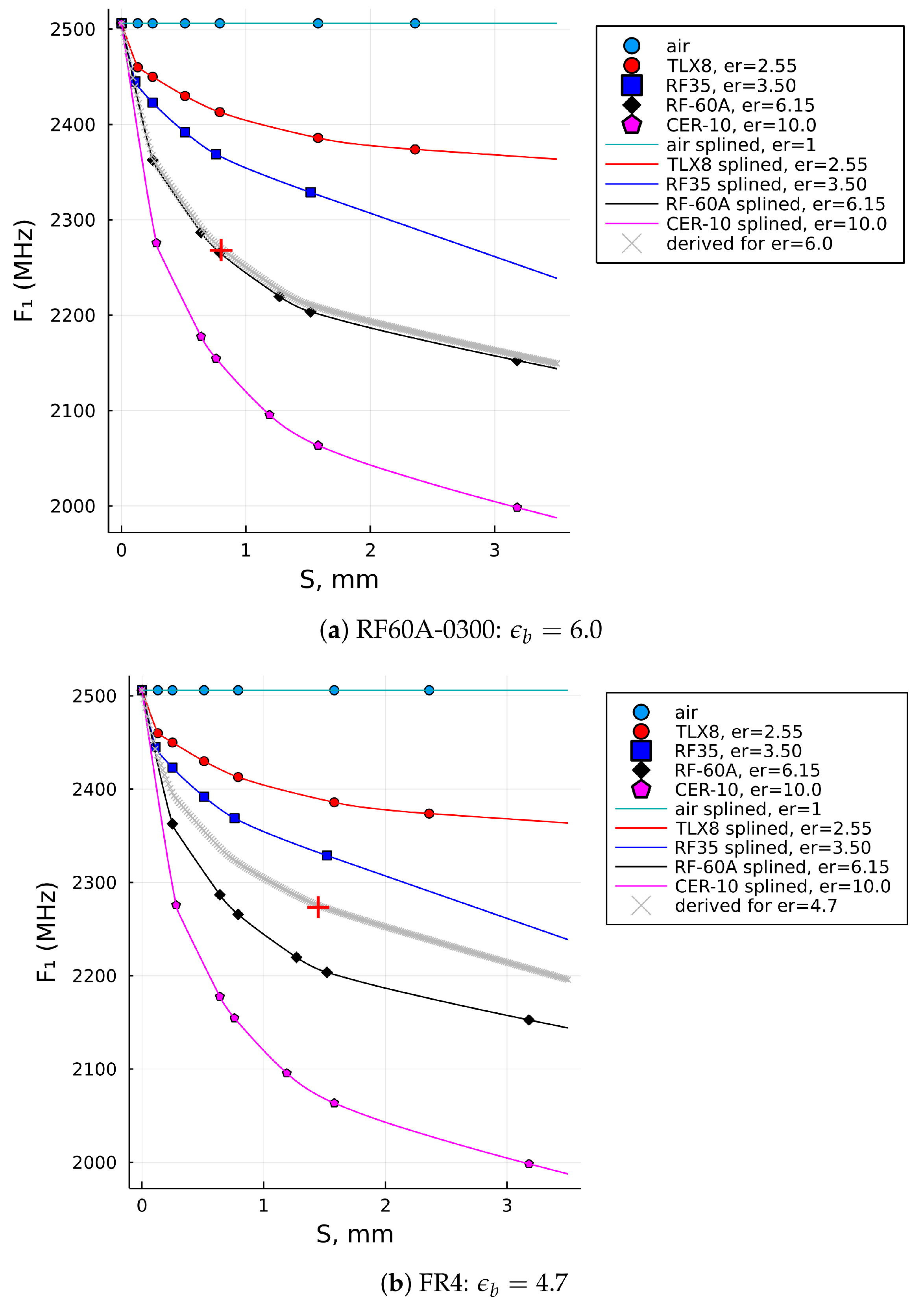
| RF60A-0300 | 0.83 | 6.15 | 2268 | 6.2 | 6.0 |
| RF60A-0620 | 1.59 | 6.15 | 2205 | 5.84 | 6.1 |
| jeans | 0.9 | 1.7 | 2447 | 1.86 | 2.0 |
| FR4 | 1.48 | 4.3–4.6 | 2276 | 4.44 | 4.7 |
| glass | 1.93 | 4–7 | 2166 | 6.28 | 6.85 |
| Plexiglass 1 | 2.95 | 2.6–3.5 | 2375 | 2.34 | 2.5 |
| Reference Laminate | Nominal Permittivity, | Laminate Thickness, S (mm) | ||||||||||||
|---|---|---|---|---|---|---|---|---|---|---|---|---|---|---|
| Initial Data Set | Extended Data Set | |||||||||||||
| TLX-8 | 2.55 | 0.13 | 0.25 | 0.51 | 0.79 | 1.58 | 2.36 | 3.00 | 3.50 | 4.00 | 5.00 | 6.00 | 7.00 | |
| RF-35 | 3.50 | 0.11 | 0.25 | 0.51 | 0.76 | 1.52 | n/a | 2.30 | 3.00 | 3.50 | 4.00 | 5.00 | 6.00 | 7.00 |
| RF-60A | 6.15 | 0.25 | 0.64 | 0.79 | 1.27 | 1.52 | 3.18 | 3.50 | 4.00 | 5.00 | 6.00 | 7.00 | ||
| CER-10 | 10.0 | 0.28 | 0.64 | 0.76 | 1.19 | 1.58 | 3.18 | 4.00 | 5.00 | 6.00 | 7.00 | |||
| SUT | S (mm) | (MHz) | by alg. in ([34], Table 7) | by this alg. (orig. data) | by this alg. (ext. data) | |
|---|---|---|---|---|---|---|
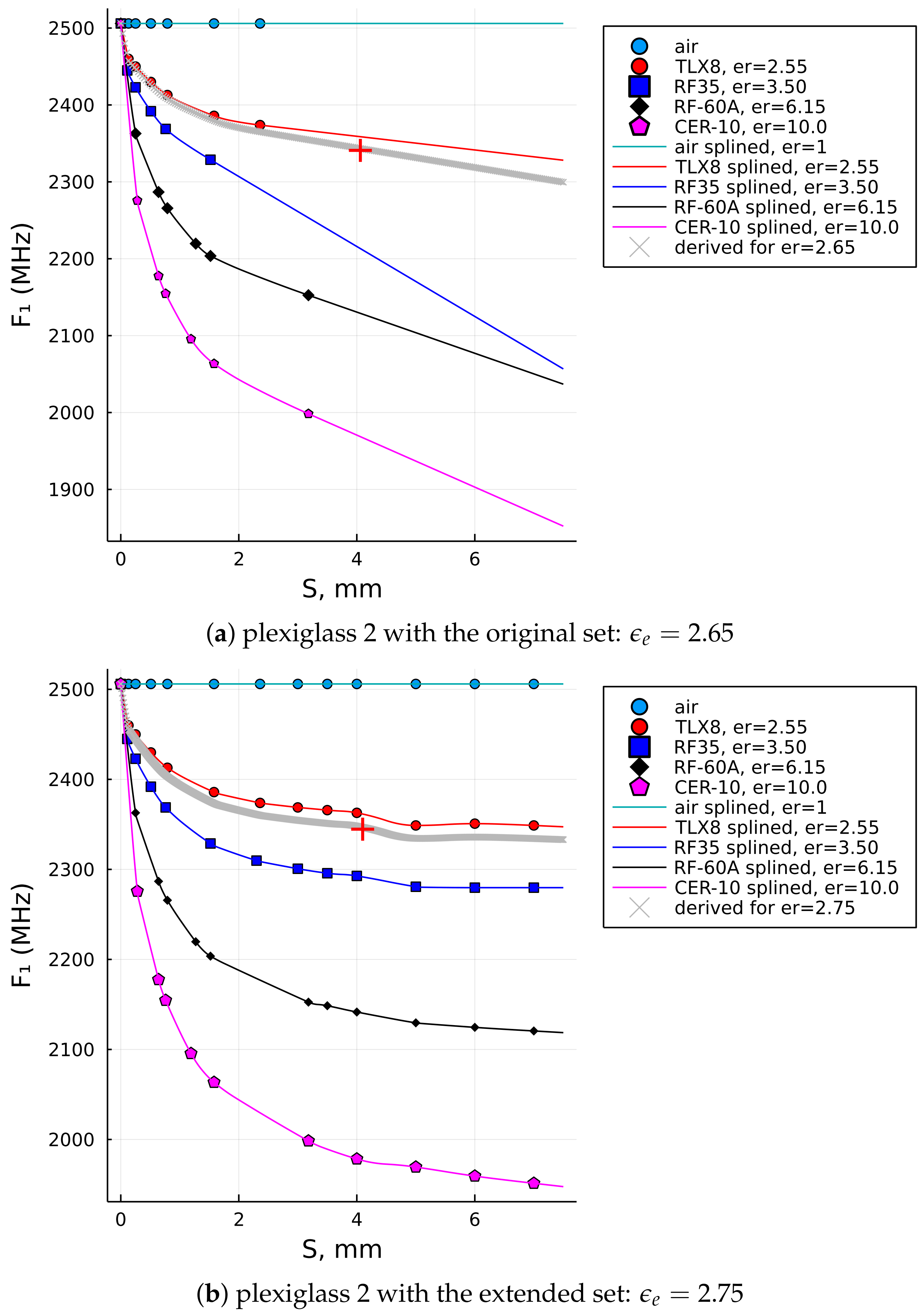
| Plexiglass 2 | 4.13 | 2.6–3.5 | 2349 | 2.57 | 2.65 | 2.75 |
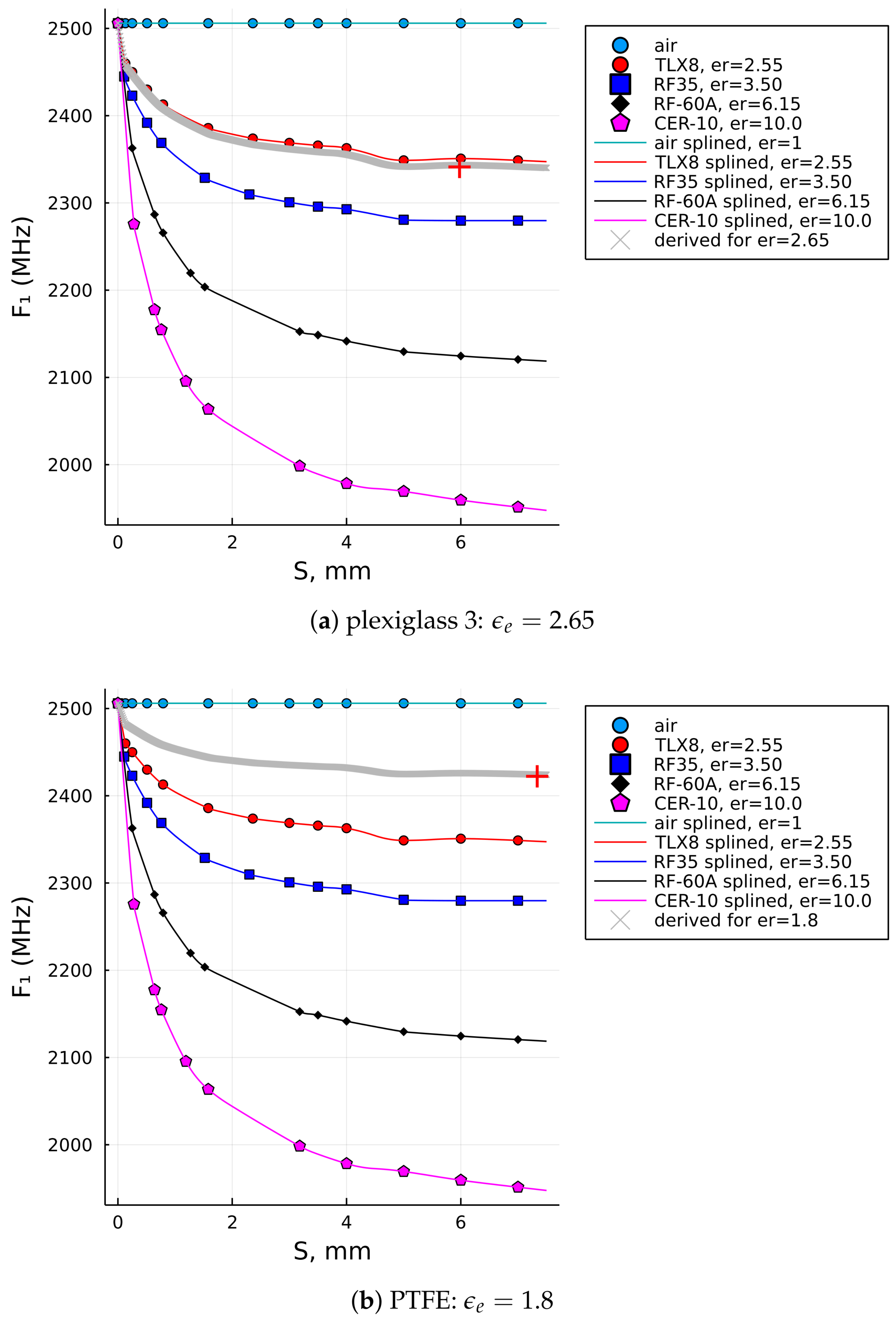
| Plexiglass 3 | 6 | 2.6–3.5 | 2349 | 2.49 | 2.5 | 2.65 |
| PTFE | 7.37 | 2 | 2428 | 1.67 | 1.7 | 1.8 |
Publisher’s Note: MDPI stays neutral with regard to jurisdictional claims in published maps and institutional affiliations. |
© 2022 by the author. Licensee MDPI, Basel, Switzerland. This article is an open access article distributed under the terms and conditions of the Creative Commons Attribution (CC BY) license (https://creativecommons.org/licenses/by/4.0/).
Share and Cite
Joler, M. An Efficient and Frequency-Scalable Algorithm for the Evaluation of Relative Permittivity Based on a Reference Data Set and a Microstrip Ring Resonator. Sensors 2022, 22, 5591. https://doi.org/10.3390/s22155591
Joler M. An Efficient and Frequency-Scalable Algorithm for the Evaluation of Relative Permittivity Based on a Reference Data Set and a Microstrip Ring Resonator. Sensors. 2022; 22(15):5591. https://doi.org/10.3390/s22155591
Chicago/Turabian StyleJoler, Miroslav. 2022. "An Efficient and Frequency-Scalable Algorithm for the Evaluation of Relative Permittivity Based on a Reference Data Set and a Microstrip Ring Resonator" Sensors 22, no. 15: 5591. https://doi.org/10.3390/s22155591
APA StyleJoler, M. (2022). An Efficient and Frequency-Scalable Algorithm for the Evaluation of Relative Permittivity Based on a Reference Data Set and a Microstrip Ring Resonator. Sensors, 22(15), 5591. https://doi.org/10.3390/s22155591