
A Novel Deep-Learning Method with Channel Attention Mechanism for Underwater Target Recognition


Abstract
:1. Introduction
2. Structure of ResNet
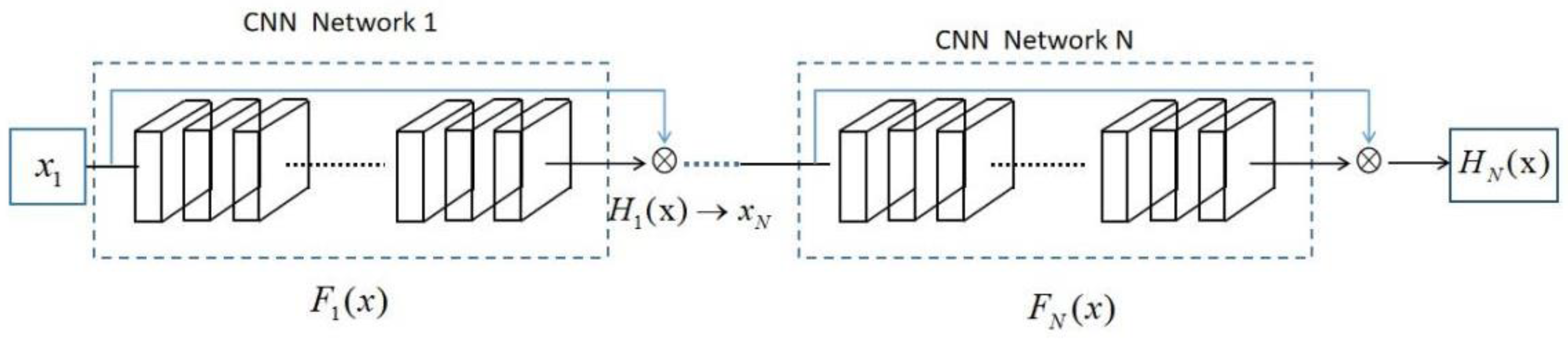
3. Architecture of camResNet in Underwater Acoustic Target Recognition Method
3.1. Architecture of camResNet
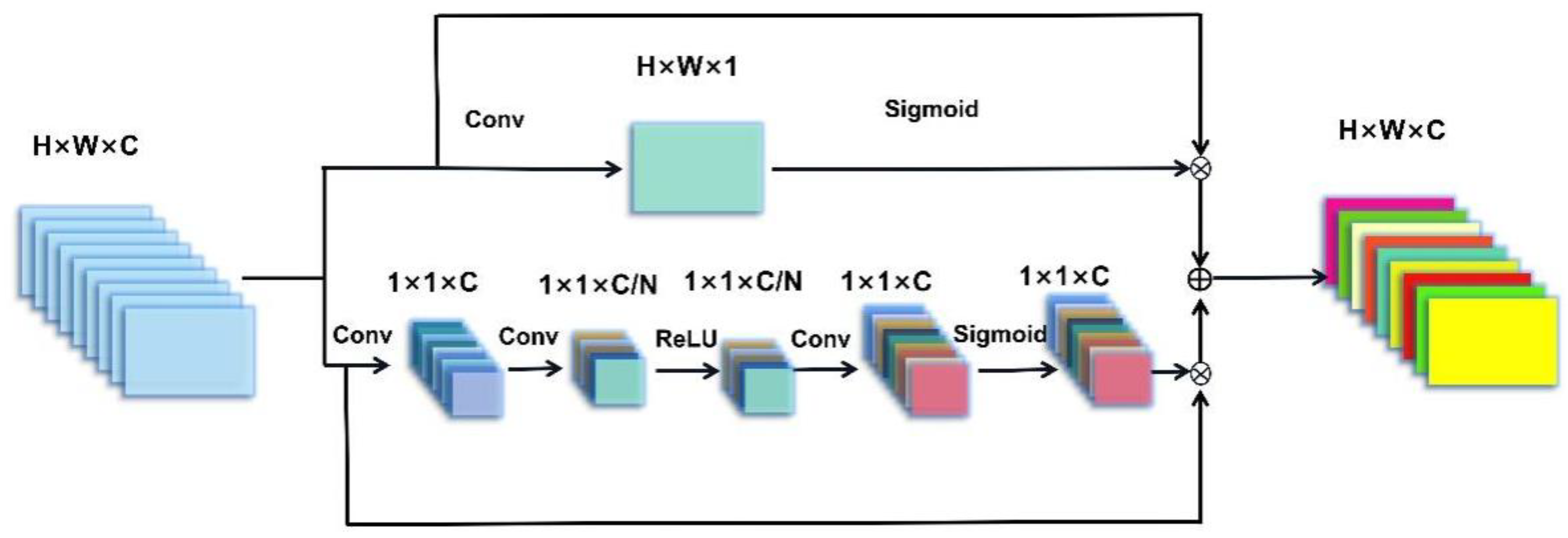
3.2. Structure of Channel Attention Mechanism Based on Underwater Acoustic of camResNet
4. Model Evaluation
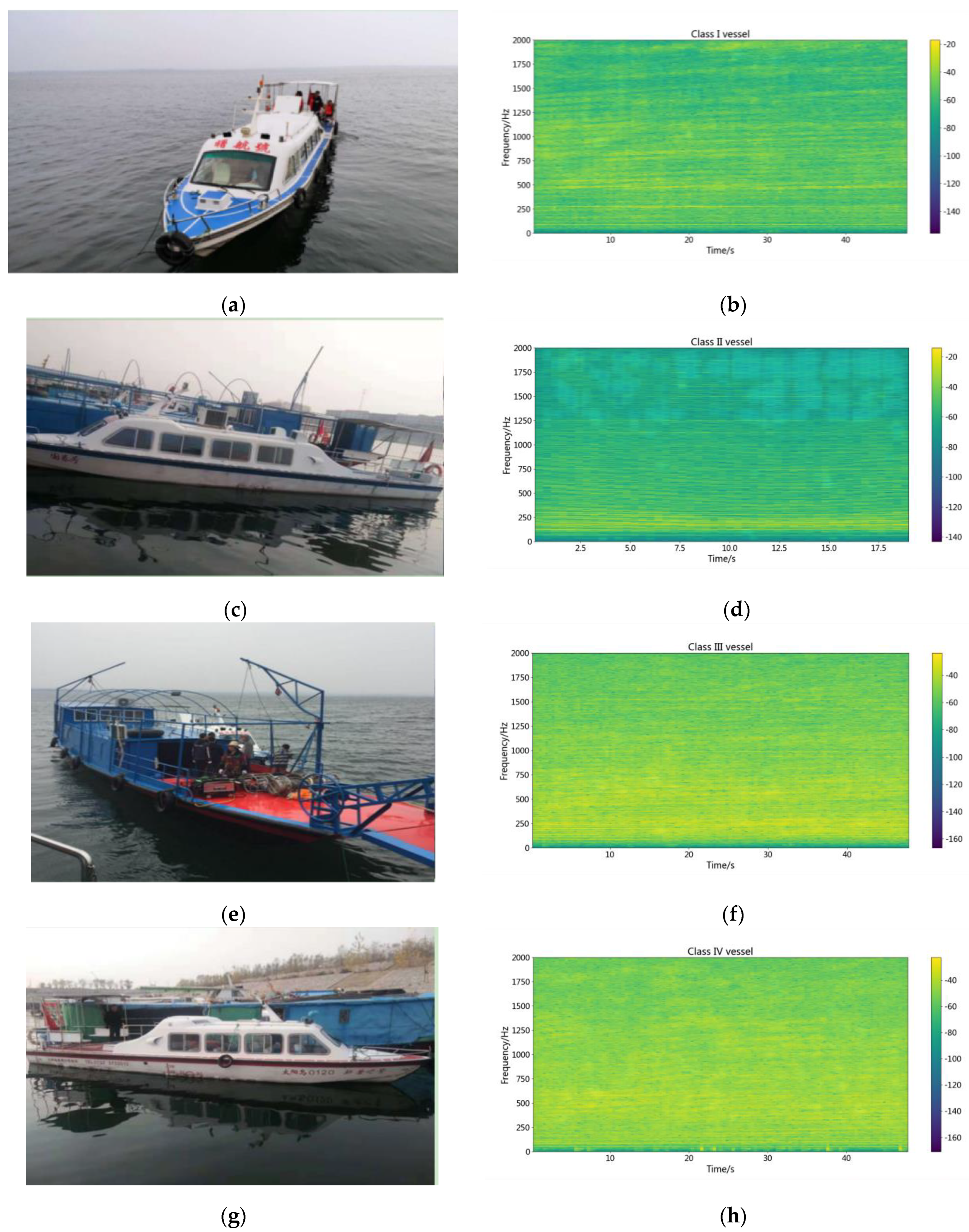
4.1. Dataset
4.2. Data Pre-Processing
4.3. Experimental Results
4.3.1. Discussion of Model Structure
4.3.2. Classification Experiment Results
- (1)
- The DBN model has an input layer, three hidden layers, and one output layer. The number of nodes in the input layer is 199, the number of nodes in the three hidden layers is 100, 50, and 20, and the number of nodes in the output layer is the number of sample categories. Each pair of adjacent layers constitutes an RBM network, and the three RBM networks are trained separately first, followed by the whole network. A batch method with a batch size of 64 is used for training. A gradient descent algorithm with a learning rate of 0.01 is used to optimize the training process.
- (2)
- The GAN network model consists of two modules: generation and discrimination. The generation module consists of three convolutional layers, and the discrimination module consists of convolutional layers. The generative module comprises three convolutional layers, with 64, 128, and 800 filters with a filter size of and a step size of 4. The discriminative model is a single-layer convolutional neural network with 16 filters with a filter size of and a step size of 4. Batch training with a batch size of 64 is used, and the learning rate is 0.001.
- (3)
- The DenseNet model is made up of three modules, each of which has three layers of a convolutional neural network. The data are normalized before each convolutional operation, and after convolution, the data are nonlinearly mapped using the elu activation function. The convolutional operation with a convolutional kernel size of and a step size of 1 is chosen. The batch method with a batch size of 64 is used for training. The optimization method is chosen during training using a gradient descent method, and the learning rate is 0.001. For optimization, the gradient descent algorithm is used.
- (4)
- The U_Net model is made up of three down-sampling modules and three up-sampling modules. Each down-sampling module contains two convolutional layers and a pooling layer of the specified size of . There is a splicing layer, a deconvolution layer, and a pooling layer with a pooling size of in each up-sampling module. The batch method is used for training, with a batch size of 64 and an optimization method of gradient descent with a learning rate of 0.001.
- (5)
- The SE ResNet network is set up and trained in the same way as the camResNet UAS model network, with the exception that the channel attention mechanism is a three-layer auto-encoder network model.
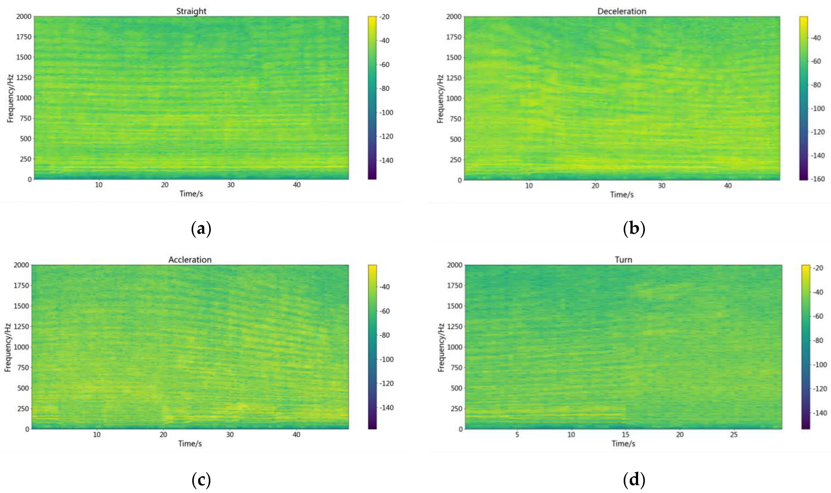
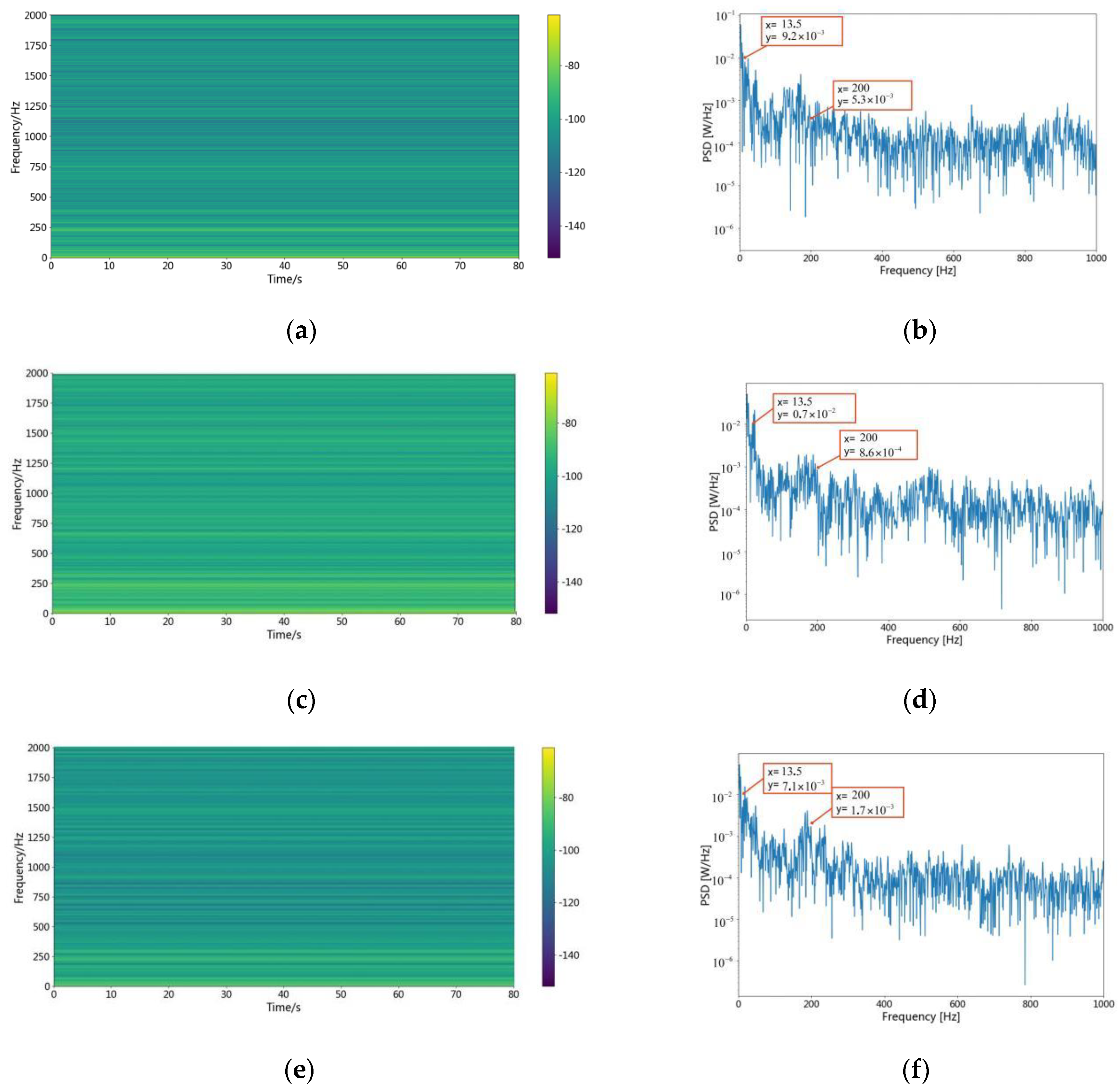
4.3.3. Visualization of Energy Distribution by the Architecture of camResNet
Power Spectral Density
t-SNE Feature Visualization Graphs
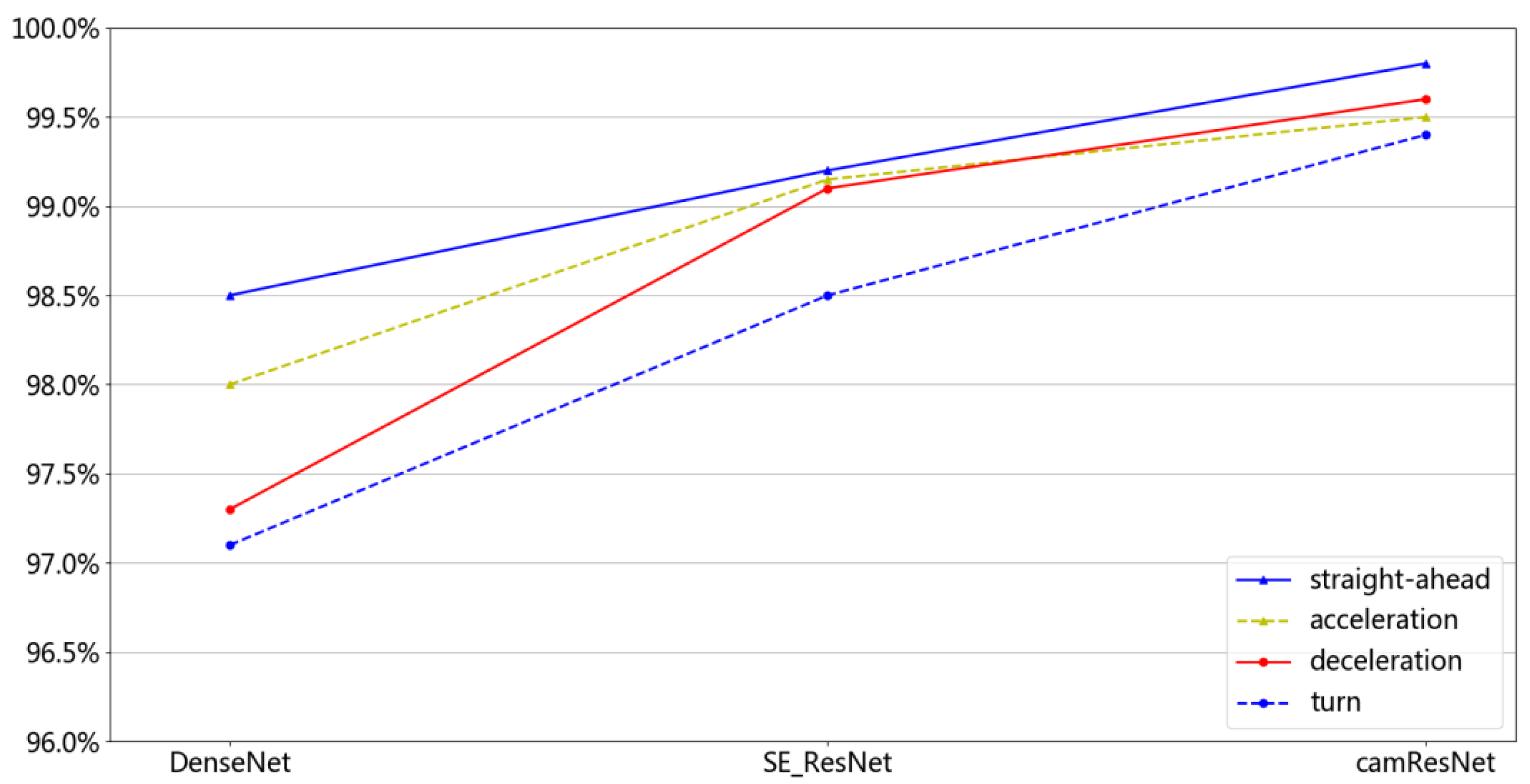
4.3.4. Recognition Results for Different Data of camResNet
- (1)
- The recognition rate of the camResNet model is higher than that of both the DenseNet model and the SE_ResNet model. The camResNet model can extract stable features that are effective for recognition.
- (2)
- The recognition rate of the camResNet model under the straight motion condition is higher than under the other conditions, which indicates that the Doppler shift can affect the recognition of camResNet.
- (3)
- There are different recognition rates with different working conditions containing different Doppler shifts. The maximum recognition rate of camResNet is 0,998; the minimum recognition rate is 0.994. The maximum recognition rate of DenseNet is 0.985, and the minimum recognition rate is 0.971. The decrease in recognition rate due to different Doppler shifts is smaller in the camResNet model than in the other models, which shows that the camResNet model has a better extraction of signals with Doppler shifts.
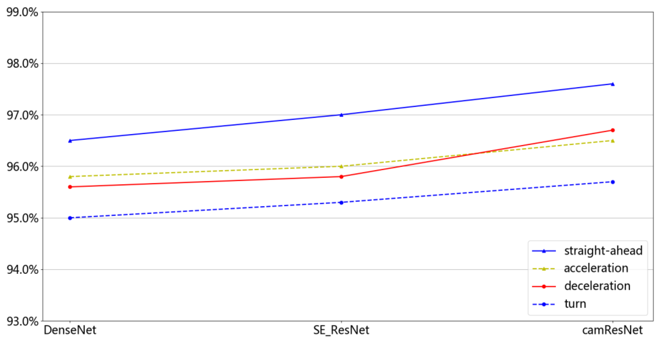
- (1)
- The maximum recognition rate of camResNet is 0,976; the minimum recognition rate is 0.965. The maximum recognition rate of DenseNet is 0.957, and the minimum recognition rate is 0.95. The recognition rate of the camResNet model is higher than that of the DenseNet model and the SE_ResNet model, and the performance is most evident under the deceleration condition.
- (2)
- The recognition rates of the three network models vary smoothly under different working conditions, indicating that all three network models can extract stable signals from the initial signals and remove unstable frequency shifts. The camResNet model has the most robust ability from the recognition results.
- (3)
- Compared with identical distributions of the training and test sets, the decrease in recognition rate due to different Doppler shifts becomes more prominent when the distributions of the training and test sets are not identical. This indicates that the recognition capabilities of the camResNet model with a Doppler shift are related to the distribution of training and test sets.
5. Conclusions
Author Contributions
Funding
Institutional Review Board Statement
Informed Consent Statement
Data Availability Statement
Conflicts of Interest
References
- Li, Y.X.; Geng, B.; Jiao, S.B. Refined Composite Multi-Scale Reverse Weighted Permutation Entropy and Its Applications in Ship-Radiated Noise. Entropy 2021, 23, 476. [Google Scholar] [CrossRef] [PubMed]
- Li, Y.X.; Geng, B.; Jiao, S.B. Dispersion Entropy-based Lempel-Ziv Complexity: A New Metric for Signal Analysis. Chaos Solitons Fractals 2022, 161, 112400. [Google Scholar] [CrossRef]
- Li, Y.X.; Mu, L.; Gao, P. Particle Swarm Optimization Fractional Slope Entropy: A New Time Series Complexity Indicator for Bearing Fault Diagnosis. Fractal Fract. 2022, 6, 345. [Google Scholar] [CrossRef]
- Li, Y.X.; Tang, B.; Yi, Y. A novel complexity-based mode feature representation for feature extraction of ship-radiated noise using VMD and slope entropy. Appl. Acoust. 2022, 196, 108899. [Google Scholar] [CrossRef]
- Li, Y.X.; Wang, L.; Yang, X.H. A Novel Linear Spectrum Frequency Feature Extraction Technique for Warship Radio Noise Based on Complete Ensemble Empirical Mode Decomposition with Adaptive Noise, Duffing Chaotic Oscillator and Weighted-Permutation Entropy. Entropy 2019, 21, 507. [Google Scholar] [CrossRef] [PubMed] [Green Version]
- Wang, L.; Wang, Q.; Zhao, L. Doppler-shift invariant feature extraction for underwater acoustic target classification. In Proceedings of the 2017 International Conference on Wireless Communications, Signal Processing and Networking (WiSPNET), Chennai, India, 22–24 May 2017; pp. 1209–1212. [Google Scholar]
- Wang, Q.; Zeng, X.Y.; Wang, L. Passive Moving Target Classification Via Spectra Multiplication Method. IEEE Signal Process. Lett. 2017, 24, 451–455. [Google Scholar] [CrossRef]
- Naderi, M.; Ha, D.V.; Nguyen, V.D.; Patzold, M. Modelling the Doppler power spectrum of non-stationary underwater acoustic channels based on Doppler measurements. In Proceedings of the OCEANS’ 17, Aberdeen, UK, 19–22 June 2017; pp. 1–6. [Google Scholar]
- Li, X.; Zhao, C.; Yu, J. Underwater Bearing-Only and Bearing-Doppler Target Tracking Based on Square Root Unscented Kalman Filter. Entropy 2019, 21, 740. [Google Scholar] [CrossRef] [PubMed] [Green Version]
- Yang, H.H.; Xu, G.H.; Yi, S.Z. A New Cooperative Deep Learning Method for Underwater Acoustic Target Recognition. In Proceedings of the OCEANS 2019—Marseille, Marseille, France, 17–20 June 2019; pp. 1–4. [Google Scholar]
- Hu, G.; Wang, K.; Liu, L. Underwater Acoustic Target Recognition Based on Depthwise Separable Convolution Neural Networks. Sensors 2021, 21, 1429. [Google Scholar] [CrossRef] [PubMed]
- Wang, Q.; Zeng, X.Y. Deep learning methods and their applications in underwater targets recognition. Tech. Acoust. 2015, 34, 138–140. [Google Scholar]
- Tian, S.; Chen, D.; Wang, H. Deep convolution stack for waveform in underwater acoustic target recognition. Sci. Rep. 2021, 11, 9614. [Google Scholar] [CrossRef]
- Hong, F.; Liu, C.; Guo, L. Underwater Acoustic Target Recognition with a Residual Network and the Optimized Feature Extraction Method. Appl. Sci. 2021, 11, 1442. [Google Scholar] [CrossRef]
- Xue, L.Z.; Zeng, X.Y. Underwater Acoustic Target Recognition Algorithm Based on Generative Adversarial Networks. Acta Armamentarii 2021, 42, 2444–2452. [Google Scholar]
- Doan, V.-S.; Huynh-The, T. Underwater Acoustic Target Classification Based on Dense Convolutional Neural Network. IEEE Geosci. Remote Sens. Lett. 2020, 99, 1–5. [Google Scholar] [CrossRef]
- Gao, Y.J.; Chen, Y.C.; Wang, F.Y. Recognition Method for Underwater Acoustic Target Based on DCGAN and DenseNet. In Proceedings of the 2020 IEEE 5th International Conference on Image, Vision and Computing (ICIVC), Beijing, China, 10–12 July 2020; pp. 15–21. [Google Scholar]
- He, K.M.; Zhang, X.Y.; Ren, S.Q. Deep Residual Learning for Image Recognition. In Proceedings of the 2016 IEEE Conference on Computer Vision and Pattern Recognition (CVPR), Las Vegas, NV, USA, 26 June–1 July 2016; pp. 770–778. [Google Scholar]
- He, K.M.; Zhang, X.Y.; Ren, S.Q. Identity Mappings in Deep Residual Networks. In Proceedings of the 2016 European Conference on Computer Vision, Amsterdam, The Netherlands, 11–14 October 2016; pp. 1–15. [Google Scholar]
- Wu, Z.; Shen, C.; Hengel, A. Wider or Deeper: Revisiting the ResNet Model for Visual Recognition. Pattern Recognit. 2019, 90, 119–133. [Google Scholar] [CrossRef] [Green Version]
- Liu, P.; Wang, G.; Qi, H. Underwater Image Enhancement With a Deep Residual Framework. IEEE Access 2019, 7, 94614–94629. [Google Scholar] [CrossRef]
- Hu, J.; Shen, L.; Sun, G. Squeeze-and-Excitation Networks. In Proceedings of the IEEE Conference on Computer Vision and Pattern Recognition (CVPR), Salt Lake City, UT, USA, 18–22 June 2018; pp. 7132–7141. [Google Scholar]
- Shen, S.; Yang, H.H.; Li, J.H. Auditory Inspired Convolutional Neural Networks for Ship Type Classification with Raw Hydrophone Data. Entropy 2018, 20, 990. [Google Scholar] [CrossRef] [PubMed] [Green Version]
- Li, J.H.; Yang, H.H. The underwater acoustic target timbre perception and recognition based on the auditory inspired deep convolutional neural network. Appl. Acoust. 2021, 182, 108210. [Google Scholar] [CrossRef]
- Arveson, P.T.; Vendittis, D.J. Radiated noise characteristics of a modern cargo ship. J. Acoust. Soc. Am. 2000, 107, 118–129. [Google Scholar] [CrossRef] [PubMed]
- Jiang, J.; Wu, Z.; Lu, J. Interpretable features for underwater acoustic target recognition. Measurement 2020, 173, 108586. [Google Scholar] [CrossRef]
- Hong, F.; Liu, C.W.; Guo, L.J. Underwater Acoustic Target Recognition with ResNet18 on ShipsEar Dataset. In Proceedings of the 2021 IEEE 4th International Conference on Electronics Technology (ICET), Chengdu, China, 7–10 May 2021; pp. 1240–1244. [Google Scholar]
- Cheng, Y.S.; Li, Z.Z. Underwater Acoustic Target Recognition, 2nd ed.; Science Press: Beijing, China, 2018; pp. 45–48. [Google Scholar]


| Residual Layers. | 1 | 2 | 3 | 4 |
|---|---|---|---|---|
| Recognition rate of test set | 96.3% | 98.2% | 96.5% | 91.4% |
| Convolution Kernels | Recognition Rate of Validated Set | Recognition Rate of Test Set |
|---|---|---|
| 91.6% | 91.1% | |
| 92.0% | 91.5% | |
| 94.3% | 92.1% | |
| 97.1% | 92.3% | |
| 98.2% | 93.1% | |
| 97.9% | 93.5% | |
| 97.8% | 95.3% | |
| 98.1% | 95.3% | |
| 98.1% | 95.9% | |
| 98.2% | 96.1% | |
| 98.3% | 96.3% | |
| 99.5% | 97.4% | |
| 99.9% | 98.2% | |
| 98.9% | 97.1% | |
| 98.3% | 96.4% | |
| 99.5% | 95.9% |
| The Input | Models | Recognition Rate | |
|---|---|---|---|
| Straight Motion Data | Four Different Working Conditions | ||
| Time domain signal | camResNet | 98.9% | 98.2% |
| Frequency domain signal | DBN | 85.6% | 82.4% |
| Time domain signal | GAN | 96.6% | 96.3% |
| Frequency domain signal | DenseNet | 97.3% | 96.1% |
| Time domain signal | U_Net | 93.9% | 93.6% |
| Time domain signal | SE_ResNet | 98.8% | 97.1% |
| Precision | Recall | F1-Score | Accuracy | |
|---|---|---|---|---|
| Class I vessel | 0.996 | 0.991 | 0.993 | 0.996 |
| Class II vessel | 0.984 | 0.981 | 0.982 | 0.991 |
| Class III vessel | 0.978 | 0.982 | 0.980 | 0.990 |
| Class IV vessel | 0.993 | 0.998 | 0.995 | 0.997 |
| Class I Vessel | Class II Vessel | Class III Vessel | Class IV Vessel | |
|---|---|---|---|---|
| Class I vessel | 1783 | 1 | 7 | 9 |
| Class II vessel | 2 | 1764 | 32 | 2 |
| Class III vessel | 3 | 24 | 1772 | 1 |
| Class IV vessel | 2 | 0 | 1 | 1769 |
Publisher’s Note: MDPI stays neutral with regard to jurisdictional claims in published maps and institutional affiliations. |
© 2022 by the authors. Licensee MDPI, Basel, Switzerland. This article is an open access article distributed under the terms and conditions of the Creative Commons Attribution (CC BY) license (https://creativecommons.org/licenses/by/4.0/).
Share and Cite
Xue, L.; Zeng, X.; Jin, A. A Novel Deep-Learning Method with Channel Attention Mechanism for Underwater Target Recognition. Sensors 2022, 22, 5492. https://doi.org/10.3390/s22155492
Xue L, Zeng X, Jin A. A Novel Deep-Learning Method with Channel Attention Mechanism for Underwater Target Recognition. Sensors. 2022; 22(15):5492. https://doi.org/10.3390/s22155492
Chicago/Turabian StyleXue, Lingzhi, Xiangyang Zeng, and Anqi Jin. 2022. "A Novel Deep-Learning Method with Channel Attention Mechanism for Underwater Target Recognition" Sensors 22, no. 15: 5492. https://doi.org/10.3390/s22155492
APA StyleXue, L., Zeng, X., & Jin, A. (2022). A Novel Deep-Learning Method with Channel Attention Mechanism for Underwater Target Recognition. Sensors, 22(15), 5492. https://doi.org/10.3390/s22155492