
High-Quality Video Watermarking Based on Deep Neural Networks and Adjustable Subsquares Properties Algorithm


Abstract
:1. Introduction
2. Literature Review
3. Proposed Method
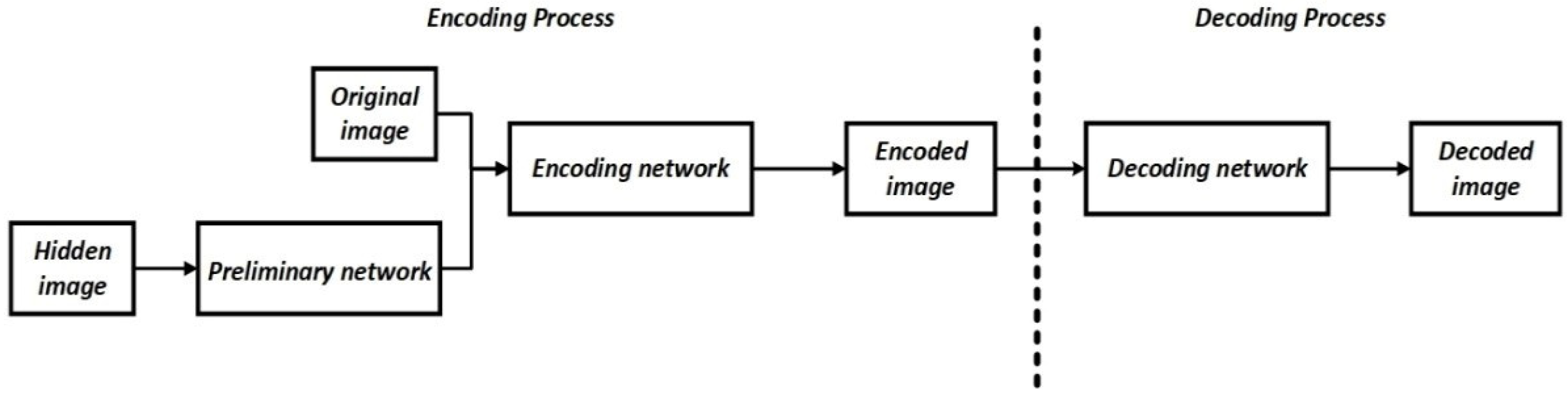
3.1. Presentation of the Concept of the Proposed Method
3.2. Adjustable Subsquares Properties Algorithm
3.3. Learning Process
3.4. Edge Effect
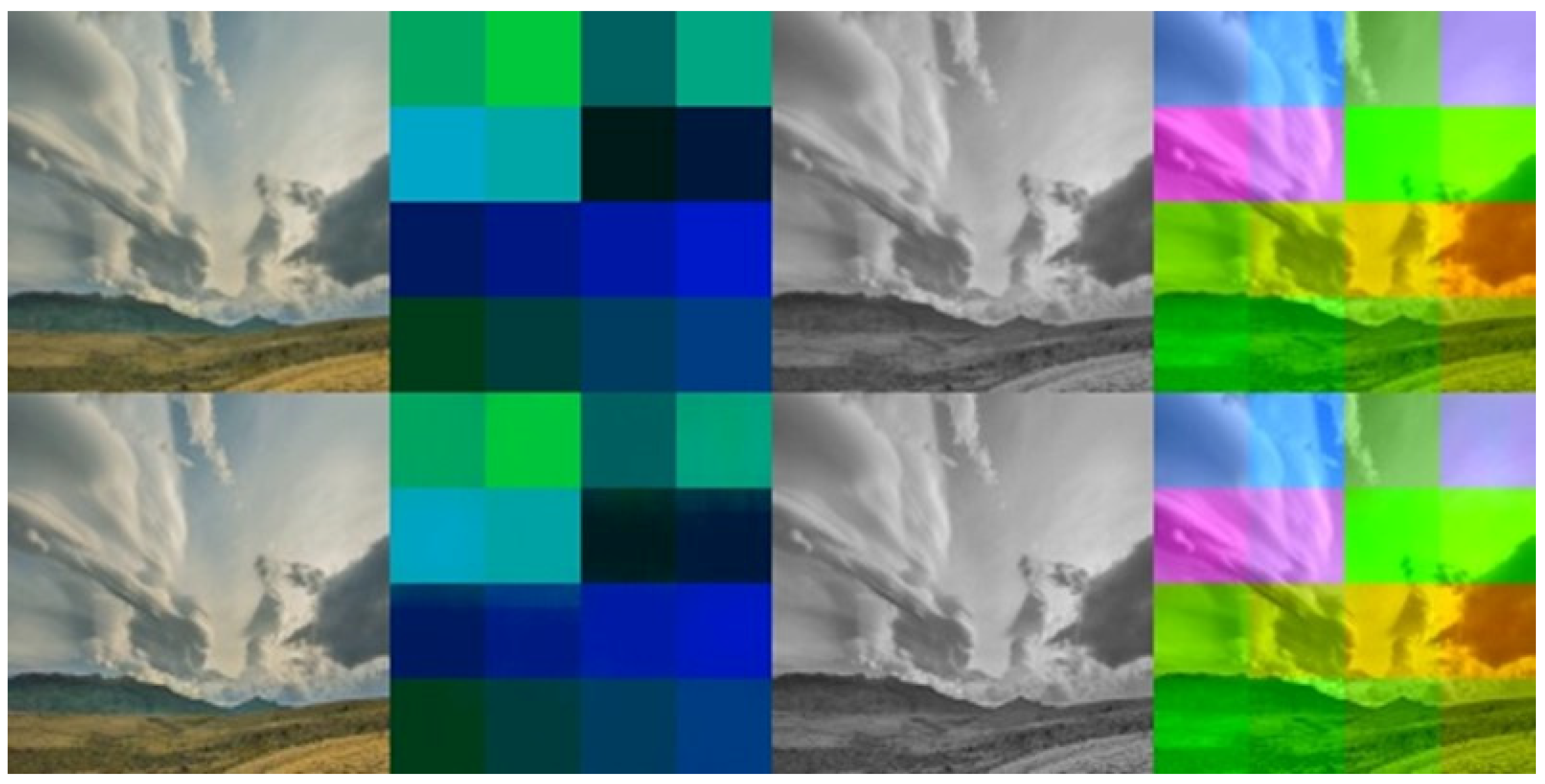
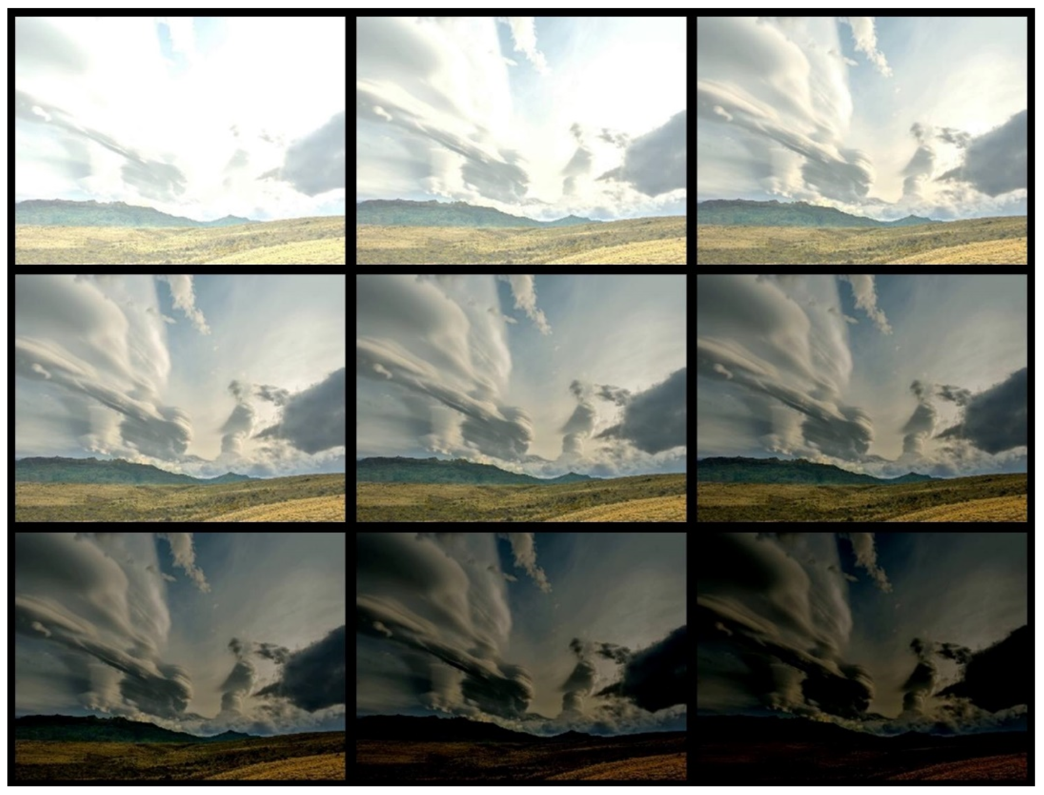
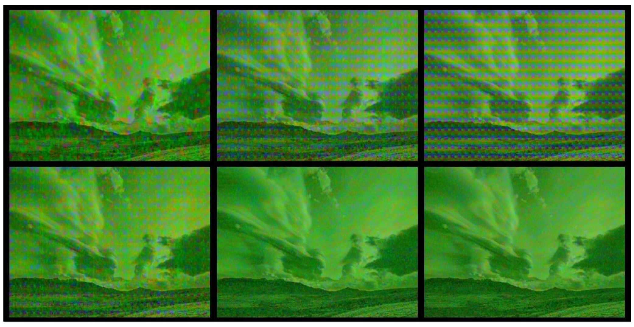
4. Results
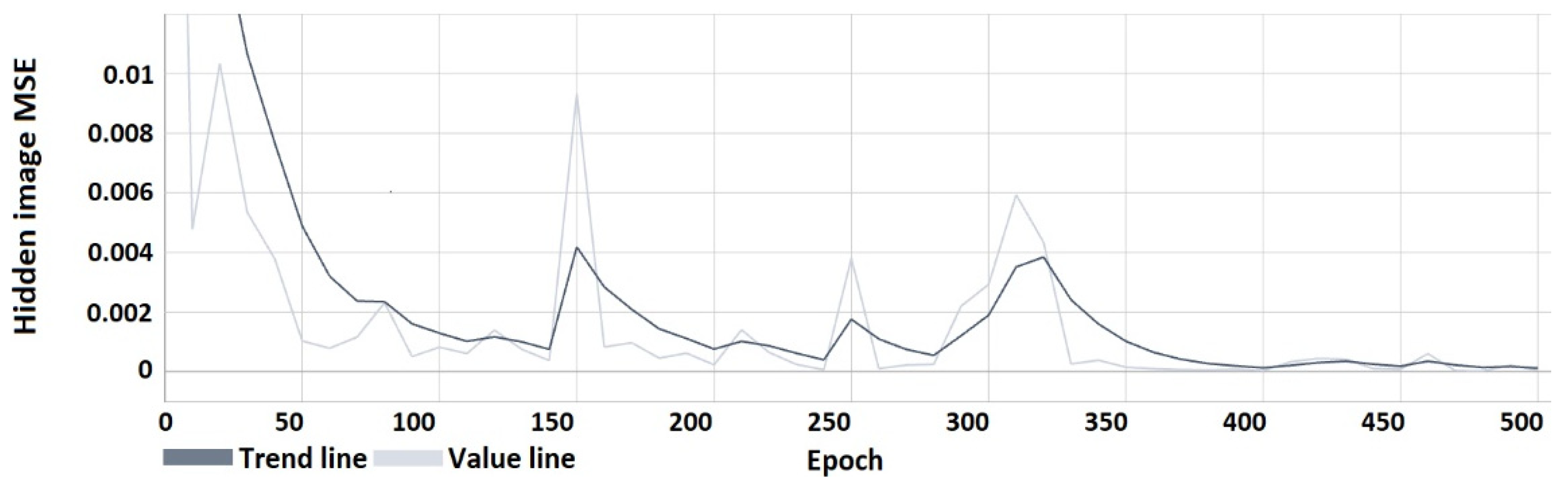
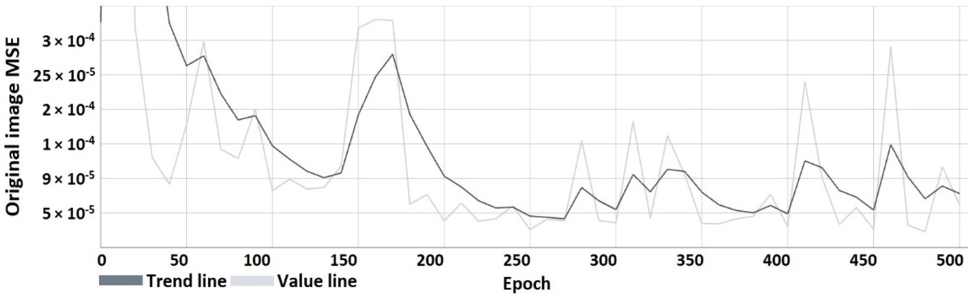
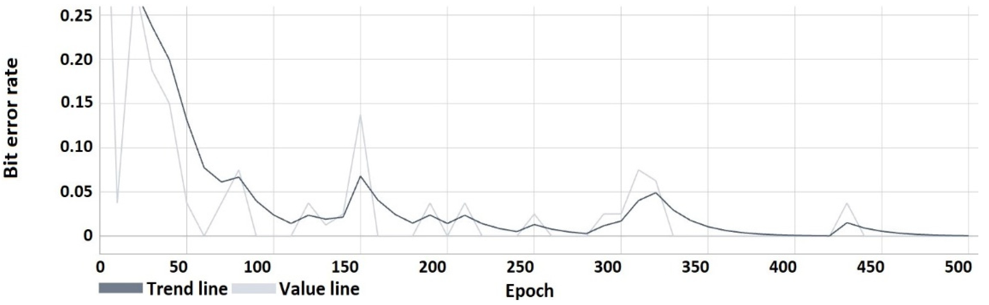
4.1. Results of the Research
4.2. Comparison with Other Methods
5. Conclusions
Author Contributions
Funding
Institutional Review Board Statement
Informed Consent Statement
Conflicts of Interest
References
- Zhang, X.; Wang, Z.; Yu, J.; Qian, Z. Reversible visible watermark embedded in encrypted domain. In Proceedings of the 2015 IEEE China Summit and International Conference on Signal and Information Processing (ChinaSIP), Chengdu, China, 12–15 July 2015; pp. 826–830. [Google Scholar] [CrossRef]
- Hu, Y.; Jeon, B. Reversible Visible Watermarking Technique for Images. In Proceedings of the 2006 International Conference on Image Processing, Atlanta, GA, USA, 8–11 October 2006; pp. 2577–2580. [Google Scholar] [CrossRef]
- Kumar, N.V.; Sreelatha, K.; Kumar, C.S. Invisible watermarking in printed images. In Proceedings of the 2016 1st India International Conference on Information Processing (IICIP), Delhi, India, 12–14 August 2016; pp. 1–5. [Google Scholar] [CrossRef]
- Chacko, S.E.; Mary, I.T.B.; Raj, W.N.D. Embedding invisible watermark in digital image using interpolation and histogram shifting. In Proceedings of the 2011 3rd International Conference on Electronics Computer Technology, Kanyakumari, India, 8–10 April 2011; pp. 89–93. [Google Scholar] [CrossRef]
- Dong, L.; Yan, Q.; Liu, M.; Pan, Y. Maximum likelihood watermark detection in absolute domain using Weibull model. In Proceedings of the 2014 IEEE Region 10 Symposium, Kuala Lumpur, Malaysia, 14–16 April 2014; pp. 196–199. [Google Scholar] [CrossRef]
- Hu, L.; Jiang, L. Blind Detection of LSB Watermarking at Low Embedding Rate in Grayscale Images. In Proceedings of the 2007 Second International Conference on Communications and Networking in China, Shanghai, China, 22–24 August 2007; pp. 413–416. [Google Scholar] [CrossRef]
- Xu, C.; Lu, Y.; Zhou, Y. An automatic visible watermark removal technique using image inpainting algorithms. In Proceedings of the 2017 4th International Conference on Systems and Informatics (ICSAI), Hangzhou, China, 11–13 November 2017; pp. 1152–1157. [Google Scholar] [CrossRef]
- Liu, Y.; Zhu, Z.; Bai, X. WDNet: Watermark-Decomposition Network for Visible Watermark Removal. In Proceedings of the 2021 IEEE Winter Conference on Applications of Computer Vision (WACV), Waikoloa, HI, USA, 3–8 January 2021; pp. 3684–3692. [Google Scholar] [CrossRef]
- An, Z.; Liu, H. Research on Digital Watermark Technology Based on LSB Algorithm. In Proceedings of the 2012 Fourth International Conference on Computational and Information Sciences, Chongqing, China, 17–19 August 2012; pp. 207–210. [Google Scholar] [CrossRef]
- Giri, K.J.; Peer, M.A.; Nagabhushan, P. A channel wise color image watermarking scheme based on Discrete Wavelet Transformation. In Proceedings of the 2014 International Conference on Computing for Sustainable Global Development (INDIACom), New Delhi, India, 5–7 March 2014; pp. 758–762. [Google Scholar] [CrossRef]
- El’arbi, M.; Amar, C.B.; Nicolas, H. Video Watermarking Based on Neural Networks. In Proceedings of the 2006 IEEE International Conference on Multimedia and Expo, Toronto, ON, Canada, 9–12 July 2006; pp. 1577–1580. [Google Scholar] [CrossRef] [Green Version]
- Mishra, A.; Agarwal, C.; Chetty, G. Lifting Wavelet Transform based Fast Watermarking of Video Summaries using Extreme Learning Machine. In Proceedings of the 2018 International Joint Conference on Neural Networks (IJCNN), Rio de Janeiro, Brazil, 8–13 July 2018; pp. 1–7. [Google Scholar] [CrossRef]
- Wagdarikar, A.M.U.; Senapati, R.K. Robust and novel blind watermarking scheme for H.264 compressed video. In Proceedings of the 2015 International Conference on Signal Processing and Communication Engineering Systems, Guntur, India, 2–3 January 2015; pp. 276–280. [Google Scholar] [CrossRef]
- Meerwald, P.; Uhl, A. Robust Watermarking of H.264-Encoded Video: Extension to SVC. In Proceedings of the 2010 Sixth International Conference on Intelligent Information Hiding and Multimedia Signal Processing, Darmstadt, Germany, 15–17 October 2010; pp. 82–85. [Google Scholar] [CrossRef]
- Zhou, Y.; Wang, C.; Zhou, X. An Intra-Drift-Free Robust Watermarking Algorithm in High Efficiency Video Coding Compressed Domain. IEEE Access 2019, 7, 132991–133007. [Google Scholar] [CrossRef]
- Gaj, S.; Sur, A.; Bora, P.K. A robust watermarking scheme against re-compression attack for H.265/HEVC. In Proceedings of the 2015 Fifth National Conference on Computer Vision, Pattern Recognition, Image Processing and Graphics (NCVPRIPG), Patna, India, 16–19 December 2015; pp. 1–4. [Google Scholar] [CrossRef]
- Nikolaidis, N.; Pitas, I. Robust image watermarking in the spatial domain. Signal Process. 1998, 66, 385–403. [Google Scholar] [CrossRef]
- Anushka; Saxena, A. Digital image watermarking using least significant bit and discrete cosine transformation. In Proceedings of the 2017 International Conference on Intelligent Computing, Instrumentation and Control Technologies (ICICICT), Kannur, India, 6–7 July 2017; pp. 1582–1586. [Google Scholar] [CrossRef]
- Lee, M.; Chang, H.; Wang, M. Watermarking Mechanism for Copyright Protection by Using the Pinned Field of the Pinned Sine Transform. In Proceedings of the 2009 10th International Symposium on Pervasive Systems, Algorithms, and Networks, Kaohsiung, Taiwan, 14–16 December 2009; pp. 502–507. [Google Scholar] [CrossRef]
- Lang, J.; Sun, J.-Y.; Yang, W.-F. A Digital Watermarking Algorithm Based on Discrete Fractional Fourier Transformation. In Proceedings of the 2012 International Conference on Computer Science and Service System, Nanjing, China, 11–13 August 2012; pp. 691–694. [Google Scholar] [CrossRef]
- Al-Afandy, K.A.; Faragallah, O.S.; El-Rabaie, E.M.; El-Samie, F.E.A.; Elmhalawy, A. A hybrid scheme for robust color image watermarking using DSWT in DCT domain. In Proceedings of the 2016 4th IEEE International Colloquium on Information Science and Technology (CiSt), Tangier, Morocco, 24–26 October 2016; pp. 444–449. [Google Scholar] [CrossRef]
- Kulkarni, T.S.; Dewan, J.H. Digital video watermarking using Hybrid wavelet transform with Cosine, Haar, Kekre, Walsh, Slant and Sine transforms. In Proceedings of the 2016 International Conference on Computing Communication Control and automation (ICCUBEA), Pune, India, 12–13 August 2016; pp. 1–5. [Google Scholar] [CrossRef]
- Hasan, N.; Islam, M.S.; Chen, W.; Kabir, M.A.; Al-Ahmadi, S. Encryption Based Image Watermarking Algorithm in 2DWT-DCT Domains. Sensors 2021, 21, 5540. [Google Scholar] [CrossRef] [PubMed]
- Li, L.; Bai, R.; Zhang, S.; Chang, C.-C.; Shi, M. Screen-Shooting Resilient Watermarking Scheme via Learned Invariant Keypoints and QT. Sensors 2021, 21, 6554. [Google Scholar] [CrossRef] [PubMed]
- Abdel-Aziz, M.M.; Hosny, K.M.; Lashin, N.A.; Fouda, M.M. Blind Watermarking of Color Medical Images Using Hadamard Transform and Fractional-Order Moments. Sensors 2021, 21, 7845. [Google Scholar] [CrossRef] [PubMed]
- Prabha, K.; Sam, I.S. An effective robust and imperceptible blind color image watermarking using WHT. J. King Saud Univ. Comput. Inf. Sci. 2022, 34, 2982–2992. [Google Scholar] [CrossRef]
- Huynh-The, T.; Hua, C.H.; Tu, N.A.; Hur, T.; Bang, J.; Kim, D.; Amin, M.B.; Kang, B.H.; Seung, H.; Lee, S. Selective bit embedding scheme for robust blind color image watermarking. Inf. Sci. 2018, 426, 1–18. [Google Scholar] [CrossRef]
- Piotrowski, Z.; Lenarczyk, P. Blind image counterwatermarking—Hidden data filter. Multimed. Tools Appl. 2017, 76, 10119–10131. [Google Scholar] [CrossRef] [Green Version]
- Yuan, Z.; Su, Q.; Liu, D.; Zhang, X. A blind image watermarking scheme combining spatial domain and frequency domain. Vis. Comput. 2020, 37, 1867–1881. [Google Scholar] [CrossRef]
- Wang, L.; Ji, H. A Watermarking Optimization Method Based on Matrix Decomposition and DWT for Multi-Size Images. Electronics 2022, 11, 2027. [Google Scholar] [CrossRef]
- Chang, Y.-F.; Tai, W.-L. Separable Reversible Watermarking in Encrypted Images for Privacy Preservation. Symmetry 2022, 14, 1336. [Google Scholar] [CrossRef]
- Faheem, Z.B.; Ali, M.; Raza, M.A.; Arslan, F.; Ali, J.; Masud, M.; Shorfuzzaman, M. Image Watermarking Scheme Using LSB and Image Gradient. Appl. Sci. 2022, 12, 4202. [Google Scholar] [CrossRef]
- Huang, T.; Xu, J.; Yang, Y.; Han, B. Robust Zero-Watermarking Algorithm for Medical Images Using Double-Tree Complex Wavelet Transform and Hessenberg Decomposition. Mathematics 2022, 10, 1154. [Google Scholar] [CrossRef]
- Bogacki, P.; Dziech, A. Analysis of New Orthogonal Transforms for Digital Watermarking. Sensors 2022, 22, 2628. [Google Scholar] [CrossRef]
- Lee, J.-E.; Seo, Y.-H.; Kim, D.-W. Convolutional Neural Network-Based Digital Image Watermarking Adaptive to the Resolution of Image and Watermark. Appl. Sci. 2020, 10, 6854. [Google Scholar] [CrossRef]
- Zhu, J.; Kaplan, R.; Johnson, J.; Fei-Fei, L. HiDDeN: Hiding data with deep networks. In Proceedings of the European Conference on Computer Vision (ECCV), Xi’an, China, 9–13 July 2018; pp. 657–672. [Google Scholar] [CrossRef] [Green Version]
- Zhong, X.; Shih, F.Y. A robust image watermarking system based on deep neural networks. arXiv 2019, arXiv:1908.11331. [Google Scholar]
- Wen, B.; Aydore, S. ROMark, a robust watermarking system using adversarial training. arXiv 2019, arXiv:1910.01221. [Google Scholar]
- Sun, Y.; Wang, J.; Huang, H.; Chen, Q. Research on scalable video watermarking algorithm based on H.264 compressed domain. Opt. Int. J. Light Electron Opt. 2020, 227, 165911. [Google Scholar] [CrossRef]
- Li, C.; Yang, Y.; Liu, K.; Tian, L. A Semi-Fragile Video Watermarking Algorithm Based on H.264/AVC. Wirel. Commun. Mob. Comput. 2020, 2020, 8848553. [Google Scholar] [CrossRef]
- Fan, D.; Zhang, X.; Kang, W.; Zhao, H.; Lv, Y. Video Watermarking Algorithm Based on NSCT, Pseudo 3D-DCT and NMF. Sensors 2022, 22, 4752. [Google Scholar] [CrossRef]
- Dhevanandhini, G.; Yamuna, G. An effective and secure video watermarking using hybrid technique. Multimed. Syst. 2021, 27, 953–967. [Google Scholar] [CrossRef]
- Liu, Y.; Zhao, H.; Liu, S.; Feng, S.; Liu, S. A Robust and Improved Visual Quality Data Hiding Method for HEVC. IEEE Access 2018, 6, 53984–53997. [Google Scholar] [CrossRef]
- Baluja, S. Hiding images in plain sight: Deep steganography. In Proceedings of the 31st International Conference on Neural Information Processing Systems (NIPS 2017), Long Beach, CA, USA, 4–9 December 2017; pp. 2066–2076. [Google Scholar]
- Zhang, Z. Improved adam optimizer for deep neural networks. In Proceedings of the 2018 IEEE/ACM 26th International Symposium on Quality of Service (IWQoS), Banff, AB, Canada, 4–6 June 2018; pp. 1–2. [Google Scholar] [CrossRef]
- LG: Spain and Patagonia. Available online: https://4kmedia.org/lg-spain-and-patagonia-uhd-4k-demo/ (accessed on 15 July 2022).
- Syahbana, Y.A.; Herman; Rahman, A.A.; Bakar, K.A. Aligned-PSNR (APSNR) for Objective Video Quality Measurement (VQM) in video stream over wireless and mobile network. In Proceedings of the 2011 World Congress on Information and Communication Technologies, Mumbai, India, 11–14 December 2011; pp. 330–335. [Google Scholar] [CrossRef]


| Digit | Value Range | RGB Value Range |
|---|---|---|
| 0 | ||
| 1 | ||
| 2 | ||
| 3 | ||
| 4 | ||
| 5 |
| No. | Character | Binary Representation | No. | Character | Binary Representation |
|---|---|---|---|---|---|
| 1 | 0 | 00000 | 19 | I | 10010 |
| 2 | 1 | 00001 | 20 | J | 10011 |
| 3 | 2 | 00001 | 21 | K | 10011 |
| 4 | 3 | 00011 | 22 | L | 10100 |
| 5 | 4 | 00100 | 23 | M | 10101 |
| 6 | 5 | 00101 | 24 | N | 10110 |
| 7 | 6 | 00110 | 25 | O | 10111 |
| 8 | 7 | 00111 | 26 | P | 11000 |
| 9 | 8 | 01000 | 27 | Q | 11001 |
| 10 | 9 | 01001 | 28 | R | 11010 |
| 11 | A | 01010 | 29 | S | 11101 |
| 12 | B | 01011 | 30 | T | 11110 |
| 13 | C | 01100 | 31 | U | 11111 |
| 14 | D | 01101 | 32 | V | |
| 15 | E | 01110 | 33 | W | |
| 16 | F | 01111 | 34 | X | |
| 17 | G | 10000 | 35 | Y | |
| 18 | H | 10001 | 36 | Z |
| Layer Number | Layer Type |
|---|---|
| 1 | Convolution 2D layer |
| 2 | Batch Normalization |
| 3 | Convolution 2D layer |
| 4 | Batch Normalization |
| 5 | Convolution 2D layer |
| 6 | Batch Normalization |
| Layer Number | Layer Type | Parameters |
|---|---|---|
| 1 | BL | activation function: LeakyReLU kernel size: 3 × 3 filter number: 61 |
| 2 | BL | activation function: LeakyReLU kernel size: 5 × 5 filter number: 61 |
| 3 | BL | activation function: LeakyReLU kernel size: 7 × 7 filter number: 61 |
| 4 | Concatenate ((1, 2, 3), axis = 3) | - |
| 5 | BL | activation function: LeakyReLU kernel size: 7 × 7 filter number: 61 |
| 6 | BL | activation function: LeakyReLU kernel size: 5 × 5 filter number: 61 |
| 7 | BL | activation function: LeakyReLU kernel size: 3 × 3 filter number: 61 |
| 8 | Concatenate ((5, 6, 7), axis = 3) | - |
| Layer Number | Layer Type | Parameters |
|---|---|---|
| 1 | BL | activation function: LeakyReLU kernel size: 3 × 3 encoder filter number: 61 decoder filter number: 71 |
| 2 | BL | activation function: LeakyReLU kernel size: 5 × 5 encoder filter number: 61 decoder filter number: 71 |
| 3 | BL | activation function: LeakyReLU kernel size: 7 × 7 encoder filter number: 61 decoder filter number: 71 |
| 4 | Concatenate ((1, 2, 3), axis = 3) | - |
| 5 | BL | activation function: LeakyReLU kernel size: 7 × 7 encoder filter number: 61 decoder filter number: 71 |
| 6 | BL | activation function: LeakyReLU kernel size: 5 × 5 encoder filter number: 61 decoder filter number: 71 |
| 7 | BL | activation function: LeakyReLU kernel size: 3 × 3 encoder filter number: 61 decoder filter number: 71 |
| 8 | Concatenate ((5, 6, 7), axis = 3) | - |
| 9 | Convolution 2D layer | activation function: LeakyReLU kernel size: 1 |
| Type | Input Tensor Size | Number of Weights | Size on Disk | Processing Time for a Single Tensor [ms] | GPU Processor |
|---|---|---|---|---|---|
| Encoder | (2, 128, 128, 3) | 6,523,953 | 75.3 MB | 106.681 | GeForce 1080Ti GTX 11GB |
| Decoder | (128, 128, 3) | 7,647,390 | 88.2 MB | 31.25 |
| Frame # | CRF 0 | CRF 1 | CRF 4 | CRF 7 | CRF 10 | CRF 13 | CRF 16 | CRF 19 | CRF 22 | CRF 23 |
|---|---|---|---|---|---|---|---|---|---|---|
| 1 | S 1: 4 | S: 4 | S: 4 | S: 3 | S: 2 | S: 3 | S: 3 | S: 2 | S: 1 | S: 1 |
| M 2: 4 | M: 4 | M: 4 | M: 3 | M: 2 | M: 3 | M: 3 | M: 2 | M: 1 | M: 1 | |
| 5 | S: 16 | S: 16 | S: 16 | S: 16 | S: 16 | S: 16 | S: 13 | S: 10 | S: 3 | S: 3 |
| M: 16 | M: 16 | M: 16 | M: 16 | M: 16 | M: 16 | M: 15 | M: 12 | M: 6 | M: 3 | |
| 10 | S: 16 | S: 16 | S: 16 | S: 16 | S: 16 | S: 16 | S: 16 | S: 13 | S: 4 | S: 2 |
| M: 16 | M: 16 | M: 16 | M: 16 | M: 16 | M: 16 | M: 16 | M: 11 | M: 4 | M: 3 | |
| 15 | S: 16 | S: 16 | S: 16 | S: 16 | S: 16 | S: 16 | S: 16 | S: 12 | S: 2 | S: 2 |
| M: 16 | M: 16 | M: 16 | M: 16 | M: 16 | M: 16 | M: 16 | M: 12 | M: 4 | M: 2 | |
| 20 | S: 16 | S: 16 | S: 16 | S: 16 | S: 16 | S: 16 | S: 16 | S: 14 | S: 2 | S: 2 |
| M: 16 | M: 16 | M: 16 | M: 16 | M: 16 | M: 16 | M: 16 | M: 12 | M: 3 | M: 2 | |
| 25 | S: 16 | S: 16 | S: 16 | S: 16 | S: 16 | S: 16 | S: 14 | S: 6 | S: 2 | S: 2 |
| M: 16 | M: 16 | M: 16 | M: 16 | M: 16 | M: 16 | M: 16 | M: 12 | M: 3 | M: 2 | |
| 30 | S: 16 | S: 16 | S: 16 | S: 16 | S: 16 | S: 16 | S: 16 | S: 11 | S: 2 | S: 2 |
| M: 16 | M: 16 | M: 16 | M: 16 | M: 16 | M: 16 | M: 16 | M: 11 | M: 2 | M: 2 |
| Frame # | CRF 0 | CRF 1 | CRF 4 | CRF 7 | CRF 10 | CRF 13 | CRF 16 | CRF 19 | CRF 22 | CRF 23 |
|---|---|---|---|---|---|---|---|---|---|---|
| 1 | BER 1: 0.4125 | BER: 0.4125 | BER: 0.4125 | BER: 0.4 | BER: 0.475 | BER: 0.375 | BER: 0.4125 | BER: 0.4625 | BER: 0.4875 | BER: 0.4625 |
| MSE 2: 6.91 × 10⁻⁸ | MSE: 6.91 × 10⁻⁸ | MSE: 6.89 × 10⁻⁸ | MSE: 8.24 × 10⁻⁷ | MSE: 7.38 × 10⁻⁸ | MSE: 1.10 × 10⁻⁷ | MSE: 1.93 × 10⁻⁷ | MSE: 3.13 × 10⁻⁷ | MSE: 4.47 × 10⁻⁷ | MSE: 5.78 × 10⁻⁷ | |
| 5 | BER: 0 | BER: 0 | BER: 0 | BER: 0 | BER: 0 | BER: 0 | BER: 0.0875 | BER: 0.1625 | BER: 0.35 | BER: 0.425 |
| MSE: 1.08 × 10⁻⁵ | MSE: 1.08 × 10⁻⁵ | MSE: 1.08 × 10⁻⁵ | MSE: 1.63 × 10⁻⁵ | MSE: 1.09 × 10⁻⁵ | MSE: 1.15 × 10⁻⁵ | MSE: 1.22 × 10⁻⁵ | MSE: 1.30 × 10⁻⁵ | MSE: 1.40 × 10⁻⁵ | MSE: 1.45 × 10⁻⁵ | |
| 10 | BER: 0 | BER: 0 | BER: 0 | BER: 0 | BER: 0 | BER: 0 | BER: 0 | BER: 0.075 | BER: 0.375 | BER: 0.45 |
| MSE: 1.16 × 10⁻⁵ | MSE: 1.16 × 10⁻⁵ | MSE: 1.16 × 10⁻⁵ | MSE: 2.08 × 10⁻⁵ | MSE: 1.18 × 10⁻⁵ | MSE: 1.26 × 10⁻⁵ | MSE: 1.35 × 10⁻⁵ | MSE: 1.48 × 10⁻⁵ | MSE: 1.65 × 10⁻⁵ | MSE: 1.72 × 10⁻⁵ | |
| 15 | BER: 0 | BER: 0 | BER: 0 | BER: 0 | BER: 0 | BER: 0 | BER: 0 | BER: 0.1125 | BER: 0.4375 | BER: 0.45 |
| MSE: 1.14 × 10⁻⁵ | MSE: 1.14 × 10⁻⁵ | MSE: 1.14 × 10⁻⁵ | MSE: 2.23 × 10⁻⁵ | MSE: 1.16 × 10⁻⁵ | MSE: 1.24 × 10⁻⁵ | MSE: 1.35 × 10⁻⁵ | MSE: 1.49 × 10⁻⁵ | MSE: 1.70 × 10⁻⁵ | MSE: 1.79 × 10⁻⁵ | |
| 20 | BER: 0 | BER: 0 | BER: 0 | BER: 0 | BER: 0 | BER: 0 | BER: 0 | BER: 0.0625 | BER: 0.4375 | BER: 0.4875 |
| MSE: 1.24 × 10⁻⁵ | MSE: 1.24 × 10⁻⁵ | MSE: 1.24 × 10⁻⁵ | MSE: 2.33 × 10⁻⁵ | MSE: 1.26 × 10⁻⁵ | MSE: 1.35 × 10⁻⁵ | MSE: 1.46 × 10⁻⁵ | MSE: 1.63 × 10⁻⁵ | MSE: 1.90 × 10⁻⁵ | MSE: 2.04 × 10⁻⁵ | |
| 25 | BER: 0 | BER: 0 | BER: 0 | BER: 0 | BER: 0 | BER: 0 | BER: 0.05 | BER: 0.3125 | BER: 0.4125 | BER: 0.5375 |
| MSE: 1.20 × 10⁻⁵ | MSE: 1.20 × 10⁻⁵ | MSE: 1.20 × 10⁻⁵ | MSE: 2.62 × 10⁻⁵ | MSE: 1.23 × 10⁻⁵ | MSE: 1.35 × 10⁻⁵ | MSE: 1.49 × 10⁻⁵ | MSE: 1.68 × 10⁻⁵ | MSE: 1.97 × 10⁻⁵ | MSE: 2.11 × 10⁻⁵ | |
| 30 | BER: 0 | BER: 0 | BER: 0 | BER: 0 | BER: 0 | BER: 0 | BER: 0 | BER: 0.15 | BER: 0.4375 | BER: 0.4625 |
| MSE: 1.23 × 10⁻⁵ | MSE: 1.23 × 10⁻⁵ | MSE: 1.23 × 10⁻⁵ | MSE: 3.02 × 10⁻⁵ | MSE: 1.26 × 10⁻⁵ | MSE: 1.37 × 10⁻⁵ | MSE: 1.50 × 10⁻⁵ | MSE: 1.71 × 10⁻⁵ | MSE: 2.11 × 10⁻⁵ | MSE: 2.30 × 10⁻⁵ |
| Frame # | CRF 7 | CRF 7 | CRF 7 | CRF 7 | CRF 7 | CRF 7 | CRF 7 | CRF 7 | CRF 7 | CRF 7 |
|---|---|---|---|---|---|---|---|---|---|---|
| BF 5 | BF 4 | BF 3 | BF 2 | BF 1 | BF −1 | BF −2 | BF −3 | BF −4 | BF −5 | |
| 1 | S: 2 | S: 2 | S: 3 | S: 4 | S: 4 | S: 1 | S: 1 | S: 1 | S: 1 | S: 1 |
| M: 2 | M: 2 | M: 3 | M: 4 | M: 4 | M: 1 | M: 1 | M: 1 | M: 1 | M: 1 | |
| 5 | S: 16 | S: 16 | S: 16 | S: 16 | S: 16 | S: 1 | S: 1 | S: 1 | S: 1 | S: 1 |
| M: 16 | M: 16 | M: 16 | M: 16 | M: 16 | M: 1 | M: 1 | M: 1 | M: 1 | M: 1 | |
| 10 | S: 16 | S: 16 | S: 16 | S: 16 | S: 16 | S: 16 | S: 1 | S: 1 | S: 1 | S: 1 |
| M: 16 | M: 16 | M: 16 | M: 16 | M: 16 | M: 1 | M: 1 | M: 1 | M: 1 | M: 1 | |
| 15 | S: 16 | S: 16 | S: 16 | S: 16 | S: 16 | S: 16 | S: 15 | S: 1 | S: 1 | S: 1 |
| M: 16 | M: 16 | M: 16 | M: 16 | M: 16 | M: 3 | M: 1 | M: 1 | M: 1 | M: 1 | |
| 20 | S: 16 | S: 16 | S: 16 | S: 16 | S: 16 | S: 16 | S: 16 | S: 3 | S: 1 | S: 1 |
| M: 16 | M: 16 | M: 16 | M: 16 | M: 16 | M: 16 | M: 1 | M: 1 | M: 1 | M: 1 | |
| 25 | S: 1 | S: 16 | S: 16 | S: 16 | S: 16 | S: 16 | S: 16 | S: 16 | S: 4 | S: 1 |
| M: 16 | M: 16 | M: 16 | M: 16 | M: 16 | M: 16 | M: 5 | M: 1 | M: 1 | M: 1 | |
| 30 | S: 1 | S: 1 | S: 5 | S: 10 | S: 11 | S: 11 | S: 8 | S: 5 | S: 4 | S: 2 |
| M: 16 | M: 16 | M: 16 | M: 16 | M: 16 | M: 16 | M: 15 | M: 1 | M: 1 | M: 1 |
| Frame # | 1080 × 1920 | 1940 × 3584 | 2032 × 3712 | 2160 × 3840 | 2288 × 3968 | 4320 × 7680 | 4608 × 8192 |
|---|---|---|---|---|---|---|---|
| 1 | S: 1 | S: 1 | S: 1 | S: 3 | S: 1 | S: 1 | S: 1 |
| M: 1 | M: 1 | M: 1 | M: 3 | M: 1 | M: 1 | M: 1 | |
| 5 | S: 1 | S: 5 | S: 4 | S: 16 | S: 3 | S: 5 | S: 5 |
| M: 1 | M: 5 | M: 5 | M: 16 | M: 4 | M: 4 | M: 5 | |
| 10 | S: 1 | S: 6 | S: 8 | S: 16 | S: 6 | S: 6 | S: 6 |
| M: 1 | M: 5 | M: 5 | M: 16 | M: 5 | M: 6 | M: 6 | |
| 15 | S: 1 | S: 7 | S: 7 | S: 16 | S: 6 | S: 8 | S: 8 |
| M: 1 | M: 7 | M: 7 | M: 16 | M: 5 | M: 6 | M: 6 | |
| 20 | S: 1 | S: 6 | S: 7 | S: 16 | S: 6 | S: 9 | S: 8 |
| M: 1 | M: 7 | M: 7 | M: 16 | M: 6 | M: 6 | M: 6 | |
| 25 | S: 1 | S: 5 | S: 5 | S: 16 | S: 6 | S: 6 | S: 7 |
| M: 1 | M: 7 | M: 7 | M: 16 | M: 6 | M: 6 | M: 6 | |
| 30 | S: 1 | S: 6 | S: 6 | S: 16 | S: 6 | S: 6 | S: 6 |
| M: 1 | M: 6 | M: 6 | M: 16 | M: 6 | M: 6 | M: 6 |
| Frame # | 1080 × 1920 | 1940 × 3584 | 2032 × 3712 | 2160 × 3840 | 2288 × 3968 | 4320 × 7680 | 4608 × 8192 |
|---|---|---|---|---|---|---|---|
| 1 | BER: 0.55 | BER: 0.55 | BER: 0.55 | BER: 0.4 | BER: 0.55 | BER: 0.55 | BER: 0.55 |
| MSE: 2.08 × 10⁻⁷ | MSE: 1.96 × 10⁻⁷ | MSE: 1.98 × 10⁻⁷ | MSE: 8.24 × 10⁻⁷ | MSE: 5.63 × 10⁻⁹ | MSE: 5.26 × 10⁻⁹ | MSE: 5.22 × 10⁻⁹ | |
| 5 | BER: 0.4875 | BER: 0.35 | BER: 0.425 | BER: 0 | BER: 0.4 | BER: 0.425 | BER: 0.375 |
| MSE: 1.09 × 10⁻⁵ | MSE: 1.07 × 10⁻⁵ | MSE: 1.06 × 10⁻⁵ | MSE: 1.63 × 10⁻⁵ | MSE: 9.77 × 10⁻⁶ | MSE: 9.64 × 10⁻⁶ | MSE: 9.67 × 10⁻⁶ | |
| 10 | BER: 0.4625 | BER: 0.3375 | BER: 0.3 | BER: 0 | BER: 0.35 | BER: 0.375 | BER: 0.3625 |
| MSE: 1.52 × 10⁻⁵ | MSE: 1.26 × 10⁻⁵ | MSE: 1.26 × 10⁻⁵ | MSE: 2.08 × 10⁻⁵ | MSE: 1.21 × 10⁻⁵ | MSE: 1.17 × 10⁻⁵ | MSE: 1.17 × 10⁻⁵ | |
| 15 | BER: 0.5125 | BER: 0.275 | BER: 0.3375 | BER: 0 | BER: 0.3625 | BER: 0.3375 | BER: 0.3 |
| MSE: 1.41 × 10⁻⁵ | MSE: 1.29 × 10⁻⁵ | MSE: 1.29 × 10⁻⁵ | MSE: 2.23 × 10⁻⁵ | MSE: 1.22 × 10⁻⁵ | MSE: 1.17 × 10⁻⁵ | MSE: 1.17 × 10⁻⁵ | |
| 20 | BER: 0.5125 | BER: 0.3 | BER: 0.3375 | BER: 0 | BER: 0.3625 | BER: 0.2625 | BER: 0.3125 |
| MSE: 1.65 × 10⁻⁵ | MSE: 1.43 × 10⁻⁵ | MSE: 1.42 × 10⁻⁵ | MSE: 2.33 × 10⁻⁵ | MSE: 1.37 × 10⁻⁵ | MSE: 1.31 × 10⁻⁵ | MSE: 1.31 × 10⁻⁵ | |
| 25 | BER: 0.5125 | BER: 0.3125 | BER: 0.375 | BER: 0 | BER: 0.375 | BER: 0.3875 | BER: 0.35 |
| MSE: 1.79 × 10⁻⁵ | MSE: 1.46 × 10⁻⁵ | MSE: 1.44 × 10⁻⁵ | MSE: 2.62 × 10⁻⁵ | MSE: 1.38 × 10⁻⁵ | MSE: 1.30 × 10⁻⁵ | MSE: 1.30 × 10⁻⁵ | |
| 30 | BER: 0.5375 | BER: 0.3 | BER: 0.3625 | BER: 0 | BER: 0.3625 | BER: 0.3875 | BER: 0.3625 |
| MSE: 2.30 × 10⁻⁵ | MSE: 1.64 × 10⁻⁵ | MSE: 1.61 × 10⁻⁵ | MSE: 3.02 × 10⁻⁵ | MSE: 1.54 × 10⁻⁵ | MSE: 1.38 × 10⁻⁵ | MSE: 1.38 × 10⁻⁵ |
| Type | Method 1 Zhou et al. [15] | Method 2 Gaj et al. [16] | Method 3 Liu et al. [43] | Proposed Method |
|---|---|---|---|---|
| Average PSNR (dB) | 47.519 | 46.415 | 45.462 | 42.617 |
| Capacity (bits/frame size) | 100 bits/ 416 × 240 | 100 bits/ 416 × 240 | 100 bits/ 416 × 240 | 80 bits/ 128 × 128 |
| Time for 20 frames of size 416 × 240 (ms) (Embedding time/Extraction time/Hardware) | 32.478/ 5.622/ 3.30 GHz CPU, 4 GB RAM | 36.855/ 5.048/ 3.30 GHz CPU, 4 GB RAM | 34.058/ 5.997/ 3.30 GHz CPU, 4 GB RAM | 34,457.92/3759.72/ Geforce 1080Ti GTX 11GB, 32 GB RAM |
Publisher’s Note: MDPI stays neutral with regard to jurisdictional claims in published maps and institutional affiliations. |
© 2022 by the authors. Licensee MDPI, Basel, Switzerland. This article is an open access article distributed under the terms and conditions of the Creative Commons Attribution (CC BY) license (https://creativecommons.org/licenses/by/4.0/).
Share and Cite
Kaczyński, M.; Piotrowski, Z. High-Quality Video Watermarking Based on Deep Neural Networks and Adjustable Subsquares Properties Algorithm. Sensors 2022, 22, 5376. https://doi.org/10.3390/s22145376
Kaczyński M, Piotrowski Z. High-Quality Video Watermarking Based on Deep Neural Networks and Adjustable Subsquares Properties Algorithm. Sensors. 2022; 22(14):5376. https://doi.org/10.3390/s22145376
Chicago/Turabian StyleKaczyński, Maciej, and Zbigniew Piotrowski. 2022. "High-Quality Video Watermarking Based on Deep Neural Networks and Adjustable Subsquares Properties Algorithm" Sensors 22, no. 14: 5376. https://doi.org/10.3390/s22145376
APA StyleKaczyński, M., & Piotrowski, Z. (2022). High-Quality Video Watermarking Based on Deep Neural Networks and Adjustable Subsquares Properties Algorithm. Sensors, 22(14), 5376. https://doi.org/10.3390/s22145376