
A Nonlinear Magnetoelastic Energy Model and Its Application in Domain Wall Velocity Prediction


Abstract
:1. Introduction
2. Model Construction
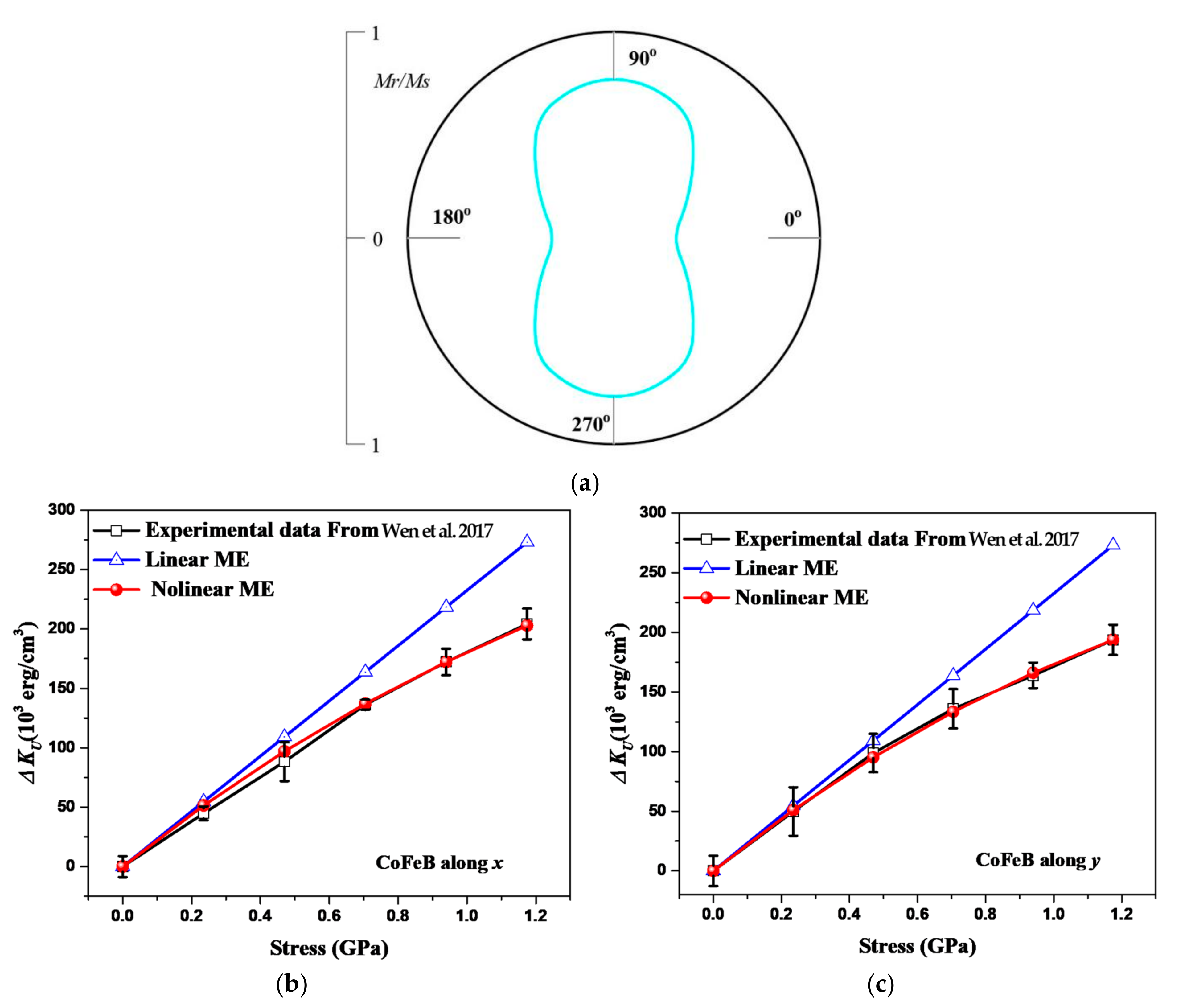
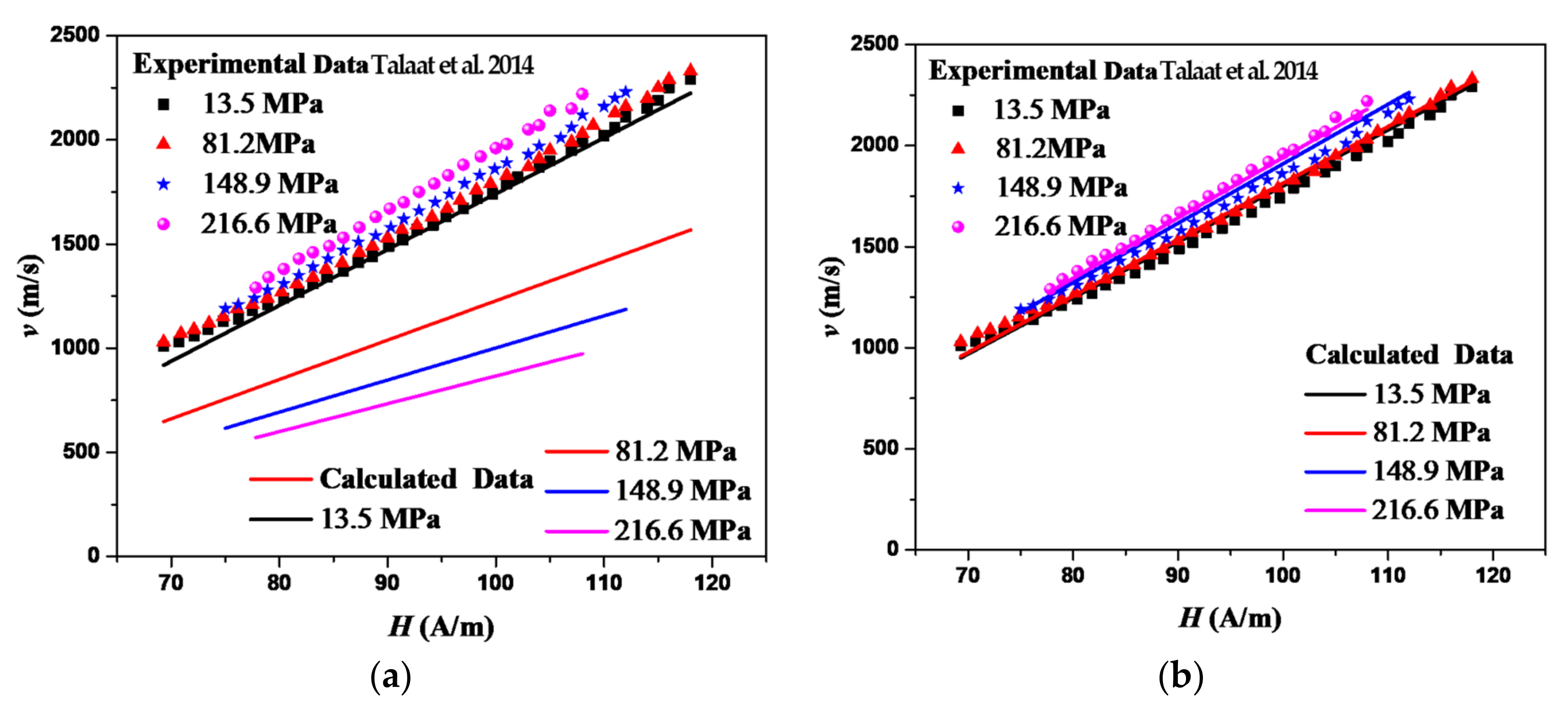
3. Model Verification
4. Model Application
5. Concluding Remarks
Author Contributions
Funding
Institutional Review Board Statement
Informed Consent Statement
Data Availability Statement
Conflicts of Interest
References
- Cornelissen, L.J.; Liu, J.; Duine, R.A.; Youssef, J.B.; van Wees, B.J. Long-distance transport of magnon spin information in a magnetic insulator at room temperature. Nat. Phys. 2015, 11, 1022. [Google Scholar] [CrossRef]
- Zhang, S.; Shi, Y.; Gao, Y. Tunability of band structures in a two-dimensional magnetostrictive phononic crystal plate with stress and magnetic loadings. Phys. Lett. A 2017, 381, 1055–1066. [Google Scholar] [CrossRef]
- Arena, D.A.; Vescovo, E.; Kao, C.C.; Guan, Y.; Bailey, W.E. Weakly coupled motion of individual layers in ferromagnetic resonance. Phys. Rev. B 2006, 74, 064409. [Google Scholar] [CrossRef] [Green Version]
- Dai, M.; Chen, X.; Sun, T.; Yu, L.; Chen, M.; Lin, H.; Chen, S. A 2D Magneto-Acousto-Electrical Tomography method to detect conductivity variation using multifocus image method. Sensors 2018, 18, 2373. [Google Scholar] [CrossRef] [Green Version]
- Saiz, P.G.; Porro, J.M.; Lasheras, A.; Luis, R.; Lopes, A.C. Influence of the magnetic domain structure in the mass sensitivity of magnetoelastic sensors with different geometries. J. Alloys Compd. 2021, 863, 158555. [Google Scholar] [CrossRef]
- Grenda, P.; Kutyła, M.; Nowicki, M.; Charubin, T. Bendductor—Transformer Steel Magnetomechanical Force Sensor. Sensors 2021, 21, 8250. [Google Scholar] [CrossRef]
- Meydan, T.; Oduncu, H. Enhancement of magnetorestrictive properties of amorphous ribbons for a biomedical application. Sens. Actuators A Phys. 1997, 59, 192–196. [Google Scholar] [CrossRef]
- Samourgkanidis, G.; Kouzoudis, D. Magnetoelastic Ribbons as Vibration Sensors for Real-Time Health Monitoring of Rotating Metal Beams. Sensors 2021, 21, 8122. [Google Scholar] [CrossRef]
- Mansourian, S.; Bakhshayeshi, A. Giant magneto-impedance variation in amorphous CoFeSiB ribbons as a function of tensile stress and frequency. Phys. Lett. A 2020, 384, 126657. [Google Scholar] [CrossRef]
- Sisniega, B.; Sagasti Sedano, A.; Gutiérrez, J.; García-Arribas, A. Real time monitoring of calcium oxalate precipitation reaction by using corrosion resistant magnetoelastic resonance sensors. Sensors 2020, 20, 2802. [Google Scholar] [CrossRef]
- Strecka, J.; Rojas, O.; Souza, S.D. Absence of a spontaneous long-range order in a mixed spin-(1/2, 3/2) ising model on a decorated square lattice due to anomalous spin frustration driven by a magnetoelastic coupling. Phys. Lett. A 2019, 383, 2451–2455. [Google Scholar] [CrossRef] [Green Version]
- Chikazumi, S.; Graham, C.D. Physics of Ferromagnetism 2e; Oxford University Press on Demand: Oxford, UK, 2009. [Google Scholar]
- Gurevich, A.G.; Melkov, G.A. Magnetization Oscillations and Waves; CRC Press: Boca Raton, FL, USA, 1996. [Google Scholar]
- Itatani, J.; Levesque, J.; Zeidler, D.; Niikura, H.; Pépin, H.; Kieffer, J.C.; Villeneuve, D.M. Tomographic imaging of molecular orbitals. Nature 2004, 432, 867–871. [Google Scholar] [CrossRef] [PubMed]
- Rana, A.; Zhang, J.; Pham, M.; Yuan, A.; Lo, Y.H.; Jiang, H.; Miao, J. Potential of attosecond coherent diffractive imaging. Phys. Rev. Lett. 2020, 125, 086101. [Google Scholar] [CrossRef] [PubMed]
- Liu, S.H. New magnetoelastic interaction. Phys. Rev. Lett. 1972, 29, 793. [Google Scholar] [CrossRef]
- Pesquera, D.; Skumryev, V.; Sanchez, F.; Herranz, G.; Fontcuberta, J. Magnetoelastic coupling in la2/3sr1/3mno3 thin films on srtio3. Phys. Rev. B 2011, 84, 184412. [Google Scholar] [CrossRef] [Green Version]
- Rinaldi, S.; Turilli, G. Theory of linear magnetoelastic effects. Phys. Rev. B 1985, 31, 3051. [Google Scholar] [CrossRef]
- Wen, X.; Wang, B.; Sheng, P.; Hu, S.; Yang, H.; Pei, K.; Li, R.W. Determination of stress-coefficient of magnetoelastic anisotropy in flexible amorphous CoFeB film by anisotropic magnetoresistance. Appl. Phys. Lett. 2017, 111, 142403. [Google Scholar] [CrossRef]
- Wang, D.; Nordman, C.; Qian, Z.; Daughton, J.M.; Myers, J. Magnetostriction effect of amorphous CoFeB thin films and application in spin-dependent tunnel junctions. J. Appl. Phys. 2005, 97, 10C906. [Google Scholar] [CrossRef]
- Hathaway, K.B.; Clark, A.E. Magnetostrictive materials. MRS Bull. 1993, 18, 34–41. [Google Scholar] [CrossRef]
- Wu, L.B.; Yao, K.; Zhao, B.X.; Wang, Y.S. A micro-statistical constructive model for magnetization and magnetostriction under applied stress and magnetic fields. Appl. Phys. Lett. 2019, 115, 162406. [Google Scholar] [CrossRef]
- Asti, G.; Bolzoni, F. Theory of first order magnetization processes: Uniaxial anisotropy. J. Magn. Magn. Mater. 1980, 20, 29–43. [Google Scholar] [CrossRef]
- Song, O. Magnetoelastic Coupling in Thin Films. Ph.D. Thesis, Massachusetts Institute of Technology, Cambridge, MA, USA, 1994. [Google Scholar]
- Tian, Z.; Sander, D.; Jürgen, K. Nonlinear magnetoelastic coupling of epitaxial layers of Fe, Co, and Ni on Ir(100). Phys. Rev. B 2009, 79, 024432. [Google Scholar] [CrossRef] [Green Version]
- Yi, M.; Xu, B.X.; Shen, Z. 180 magnetization switching in nanocylinders by a mechanical strain. Extrem. Mech. Lett. 2015, 3, 66–71. [Google Scholar] [CrossRef]
- Tang, Z.H.; Jiang, Z.S.; Chen, T.; Lei, D.J.; Yan, W.Y.; Qiu, F.; Huang, J.-Q.; Deng, H.-M.; Yao, M. Simultaneous microwave photonic and phononic band gaps in piezoelectric–piezomagnetic superlattices with three types of domains in a unit cell. Phys. Lett. A 2016, 380, 1757–1762. [Google Scholar] [CrossRef]
- Talaat, A.; Blanco, J.M.; Ipatov, M.; Zhukova, V.; Zhukov, A.P. Domain wall propagation in Co-based glass-coated microwires: Effect of stress annealing and tensile applied stresses. IEEE Trans. Magn. 2014, 50, 1–4. [Google Scholar] [CrossRef]
- Moubah, R.; Magnus, F.; Kapaklis, V.; Hjörvarsson, B.; Andersson, G. Anisotropic Magnetostriction and Domain Wall Motion in Sm10Co90 Amorphous Films. Appl. Phys. Express 2013, 6, 053004. [Google Scholar] [CrossRef]

Publisher’s Note: MDPI stays neutral with regard to jurisdictional claims in published maps and institutional affiliations. |
© 2022 by the authors. Licensee MDPI, Basel, Switzerland. This article is an open access article distributed under the terms and conditions of the Creative Commons Attribution (CC BY) license (https://creativecommons.org/licenses/by/4.0/).
Share and Cite
Wu, L.-B.; Fan, Y.-F.; Sun, F.-B.; Yao, K.; Wang, Y.-S. A Nonlinear Magnetoelastic Energy Model and Its Application in Domain Wall Velocity Prediction. Sensors 2022, 22, 5371. https://doi.org/10.3390/s22145371
Wu L-B, Fan Y-F, Sun F-B, Yao K, Wang Y-S. A Nonlinear Magnetoelastic Energy Model and Its Application in Domain Wall Velocity Prediction. Sensors. 2022; 22(14):5371. https://doi.org/10.3390/s22145371
Chicago/Turabian StyleWu, Li-Bo, Yu-Feng Fan, Feng-Bo Sun, Kai Yao, and Yue-Sheng Wang. 2022. "A Nonlinear Magnetoelastic Energy Model and Its Application in Domain Wall Velocity Prediction" Sensors 22, no. 14: 5371. https://doi.org/10.3390/s22145371
APA StyleWu, L.-B., Fan, Y.-F., Sun, F.-B., Yao, K., & Wang, Y.-S. (2022). A Nonlinear Magnetoelastic Energy Model and Its Application in Domain Wall Velocity Prediction. Sensors, 22(14), 5371. https://doi.org/10.3390/s22145371