
A Statistical Approach for A-Posteriori Deployment of Microclimate Sensors in Museums: A Case Study

 ,
,  ,
, 
 ,
,  ,
, 
Abstract
:1. Introduction
1.1. Scientific Literature about Deployment of Microclimate Sensors
1.2. Research Aims
2. Materials and Methods
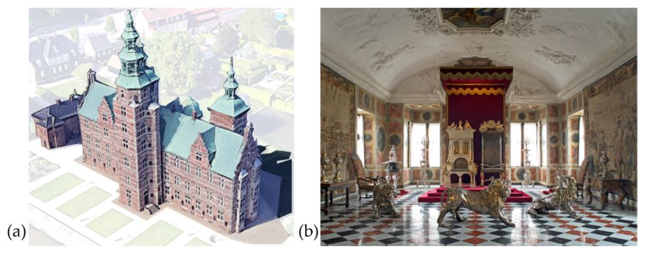
2.1. The Case Study: Rosenborg Castle
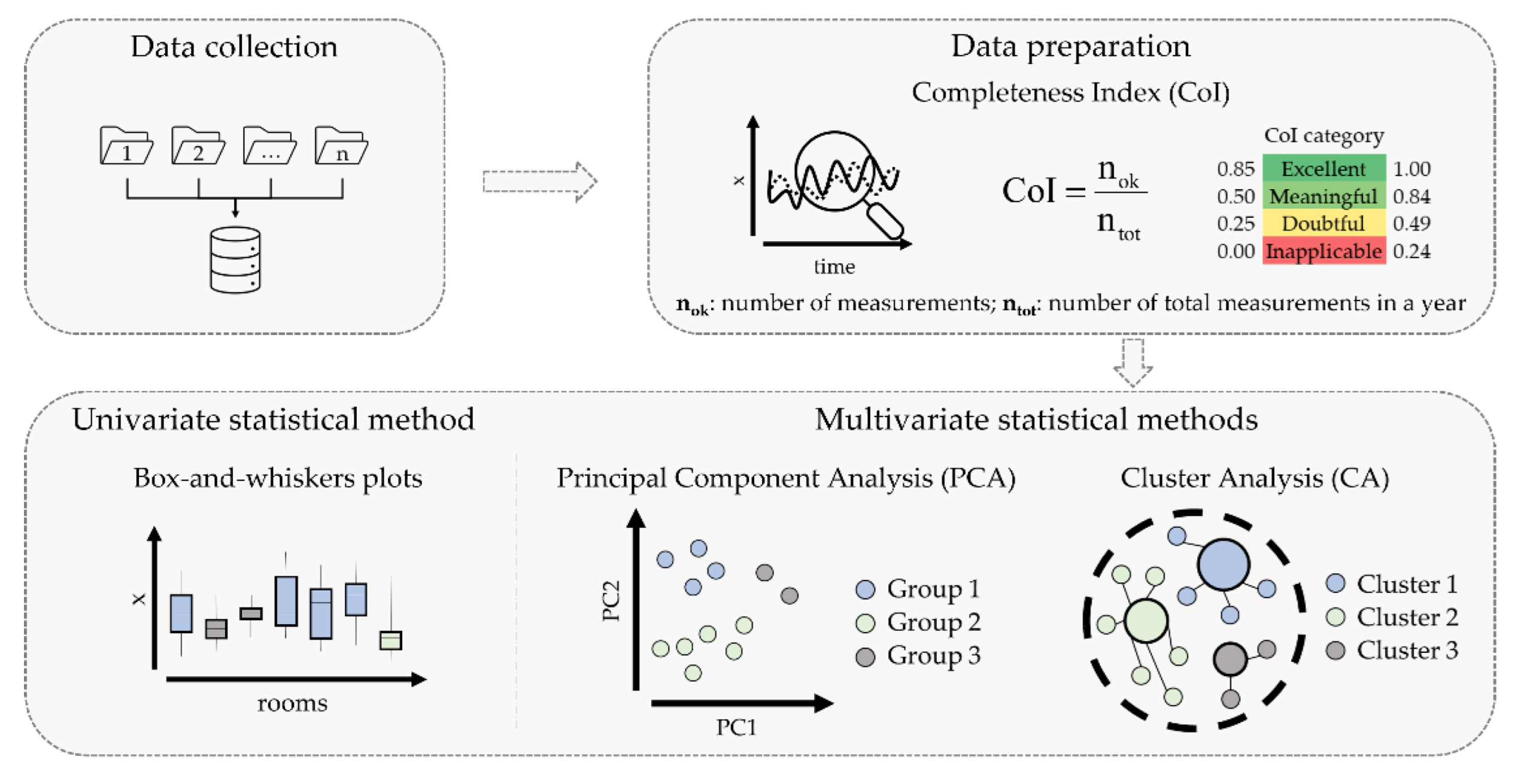
2.2. Microclimate Statistical Data Analysis
- Data preparation (Section 2.2.1): selection of a continuous long-term TRH time series (at least one calendar year).
- Application of the statistical methods:
- univariate statistics (Section 2.2.2): box-and-whisker plots;
- multivariate statistics (Section 2.2.3): cluster analysis (CA) and principal component analysis (PCA).
2.2.1. Data Preparation
2.2.2. Univariate Statistical Method
2.2.3. Multivariate Statistical Methods
3. Results
3.1. Data Pre-Processing
3.2. Univariate Statistical Method
3.3. Multivariate Statistical Methods
3.4. A-Posteriori Deployment of Microclimate Sensors
4. Conclusions
Author Contributions
Funding
Data Availability Statement
Acknowledgments
Conflicts of Interest
References
- Perles, A.; Fuster-López, L.; García-Diego, F.J.; Peiró-Vitoria, A.; García-Castillo, A.M.; Andersen, C.K.; Bosco, E.; Mavrikas, E.; Pariente, T. CollectionCare: An affordable service for the preventive conservation monitoring of single cultural artefacts during display, storage, handling and transport. IOP Conf. Ser. Mater. Sci. Eng. 2020, 949, 012026. [Google Scholar] [CrossRef]
- Camuffo, D.; Van Grieken, R.; Busse, H.J.; Sturaro, G.; Valentino, A.; Bernardi, A.; Blades, N.; Shooter, D.; Gysels, K.; Deutsch, F.; et al. Environmental monitoring in four European museums. Atmos. Environ. 2001, 35, S127–S140. [Google Scholar] [CrossRef]
- Camuffo, D. Microclimate for Cultural Heritage; Elsevier: Amsterdam, The Netherlands, 2019; ISBN 9780444632968. [Google Scholar]
- Verticchio, E.; Frasca, F.; Bertolin, C.; Siani, A.M. Climate-induced risk for the preservation of paper collections: Comparative study among three historic libraries in Italy. Build. Environ. 2021, 206, 108394. [Google Scholar] [CrossRef]
- WMO. Guide to the Global Observing System; WMO: Geneva, Switzerland, 2017; ISBN 9789263104885. [Google Scholar]
- EN 15758:2010; Conservation of Cultural Property—Procedures and Instruments for Measuring Temperatures of the Air and the Surfaces of Objects. European Committee for Standardization: Brussels, Belgium, 2010.
- EN 16242:2012; Conservation of cultural heritage—Procedures and Instruments for Measuring Humidity in the Air and Moisture Exchanges between Air and Cultural Property. European Committee for Standardization: Brussels, Belgium, 2012.
- Huijbregts, Z.; Schellen, H.; van Schijndel, J.; Ankersmit, B. Modelling of heat and moisture induced strain to assess the impact of present and historical indoor climate conditions on mechanical degradation of a wooden cabinet. J. Cult. Herit. 2015, 16, 419–427. [Google Scholar] [CrossRef]
- Muñoz-González, C.M.; León-Rodríguez, A.L.; Navarro-Casas, J. Air conditioning and passive environmental techniques in historic churches in Mediterranean climate. A proposed method to assess damage risk and thermal comfort pre-intervention, simulation-based. Energy Build. 2016, 130, 567–577. [Google Scholar] [CrossRef]
- Silva, H.E.; Coelho, G.B.A.; Henriques, F.M.A. Climate monitoring in World Heritage List buildings with low-cost data loggers: The case of the Jerónimos Monastery in Lisbon (Portugal). J. Build. Eng. 2020, 28, 101029. [Google Scholar] [CrossRef]
- Peralta, L.M.R.; Brito, L.M.P.L.; Gouveia, B.A.T.; Sousa, D.J.G.; Alves, C.S. Automatic monitoring and control of museums ’ environment based on Wireless Sensor Networks. Electron. J. Struct. Eng. 2010, 1, 12–35. [Google Scholar]
- Agbota, H.; Mitchell, J.E.; Odlyha, M.; Strlič, M. Remote assessment of cultural heritage environments with wireless sensor array networks. Sensors 2014, 14, 8779–8793. [Google Scholar] [CrossRef] [Green Version]
- Verticchio, E.; Frasca, F.; Cavalieri, P.; Teodonio, L.; Fugaro, D.; Siani, A.M. Conservation risks for paper collections induced by the microclimate in the repository of the Alessandrina Library in Rome (Italy). Herit. Sci. 2022, 10, 80. [Google Scholar] [CrossRef]
- Merello, P.; García-Diego, F.J.; Zarzo, M. Microclimate monitoring of Ariadne’s house (Pompeii, Italy) for preventive conservation of fresco paintings. Chem. Cent. J. 2012, 6, 145. [Google Scholar] [CrossRef] [Green Version]
- Visco, G.; Plattner, S.H.; Fortini, P.; Di Giovanni, S.; Sammartino, M.P. Microclimate monitoring in the Carcer Tullianum: Temporal and spatial correlation and gradients evidenced by multivariate analysis; first campaign. Chem. Cent. J. 2012, 6, S11. [Google Scholar] [CrossRef] [PubMed] [Green Version]
- Aste, N.; Adhikari, R.S.; Buzzetti, M.; Della Torre, S.; Del Pero, C.; Huerto-Cardenas, H.E.; Leonforte, F. Microclimatic monitoring of the Duomo (Milan Cathedral): Risks-based analysis for the conservation of its cultural heritage. Build. Environ. 2019, 148, 240–257. [Google Scholar] [CrossRef]
- Lucero-Gómez, P.; Balliana, E.; Farinelli, V.; Salvini, S.; Signorelli, L.; Zendri, E. Rethinking and evaluating the role of historical buildings in the preservation of fragile artworks: The case study of the Gallerie dell’Accademia in Venice. Eur. Phys. J. Plus 2022, 137, 150. [Google Scholar] [CrossRef]
- Lucchi, E.; Dias Pereira, L.; Andreotti, M.; Malaguti, R.; Cennamo, D.; Calzolari, M.; Frighi, V. Development of a Compatible, Low Cost and High Accurate Conservation Remote Sensing Technology for the Hygrothermal Assessment of Historic Walls. Electronics 2019, 8, 643. [Google Scholar] [CrossRef] [Green Version]
- Becherini, F.; Bernardi, A.; Di Tuccio, M.C.; Vivarelli, A.; Pockelè, L.; De Grandi, S.; Fortuna, S.; Quendolo, A. Microclimatic monitoring for the investigation of the different state of conservation of the stucco statues of the Longobard Temple in Cividale del Friuli (Udine, Italy). J. Cult. Herit. 2016, 18, 375–379. [Google Scholar] [CrossRef]
- Siani, A.M.; Frasca, F.; Di Michele, M.; Bonacquisti, V.; Fazio, E. Cluster analysis of microclimate data to optimize the number of sensors for the assessment of indoor environment within museums. Environ. Sci. Pollut. Res. 2018, 25, 28787. [Google Scholar] [CrossRef]
- Ramírez, S.; Zarzo, M.; García-Diego, F.J. Multivariate time series analysis of temperatures in the archaeological museum of l’Almoina (Valencia, Spain). Sensors 2021, 21, 4377. [Google Scholar] [CrossRef]
- García-Diego, F.-J.; Verticchio, E.; Beltrán, P.; Siani, A. Assessment of the minimum sampling frequency to avoid measurement redundancy in microclimate field surveys in museum buildings. Sensors 2016, 16, 1291. [Google Scholar] [CrossRef]
- Frasca, F.; Siani, A.M.; Casale, G.R.; Pedone, M.; Bratasz, Ł.; Strojecki, M.; Mleczkowska, A. Assessment of indoor climate of Mogiła Abbey in Kraków (Poland) and the application of the analogues method to predict microclimate indoor conditions. Environ. Sci. Pollut. Res. 2017, 24, 13895–13907. [Google Scholar] [CrossRef] [PubMed]
- Hersbach, H.; Bell, B.; Berrisford, P.; Biavati, G.; Horányi, A.; Muñoz Sabater, J.; Nicolas, J.; Peubey, C.; Radu, R.; Rozum, I.; et al. ERA5 hourly data on pressure levels from 1979 to present. Copernicus Clim. Chang. Serv. Clim. Data Store 2018. [Google Scholar] [CrossRef]
- Dunia, R.; Qin, S.J.; Edgar, T.F.; McAvoy, T.J. Use of principal component analysis for sensor fault identification. Comput. Chem. Eng. 1996, 20, 713–718. [Google Scholar] [CrossRef]
- Zhu, D.; Bai, J.; Yang, S.X. A multi-fault diagnosis method for sensor systems based on principle component analysis. Sensors 2010, 10, 241–253. [Google Scholar] [CrossRef] [PubMed]
- Valero, M.Á.; Merello, P.; Navajas, Á.F.; García-Diego, F.J. Statistical tools applied in the characterisation and evaluation of a thermo-hygrometric corrective action carried out at the Noheda archaeological site (Noheda, Spain). Sensors 2014, 14, 1665–1679. [Google Scholar] [CrossRef] [PubMed]
- García-Diego, F.J.; Zarzo, M. Microclimate monitoring by multivariate statistical control: The renaissance frescoes of the Cathedral of Valencia (Spain). J. Cult. Herit. 2010, 11, 339–344. [Google Scholar] [CrossRef]
- Zarzo, M.; Fernández-Navajas, A.; García-Diego, F.J. Long-term monitoring of fresco paintings in the cathedral of Valencia (Spain) through humidity and temperature sensors in various locations for preventive conservation. Sensors 2011, 11, 8685–8710. [Google Scholar] [CrossRef]
- Warren Liao, T. Clustering of time series data—A survey. Pattern Recognit. 2005, 38, 1857–1874. [Google Scholar] [CrossRef]
- Rousseeuw, P.J. Silhouettes: A graphical aid to the interpretation and validation of cluster analysis. J. Comput. Appl. Math. 1987, 20, 53–65. [Google Scholar] [CrossRef] [Green Version]
- Bile, A.; Tari, H.; Grinde, A.; Frasca, F.; Siani, A.M.; Fazio, E. Novel Model Based on Artificial Neural Networks to Predict Short-Term Temperature Evolution in Museum Environment. Sensors 2022, 22, 615. [Google Scholar] [CrossRef]


| Temperature | Relative Humidity | |
|---|---|---|
| Sensor Type | Thermistor | Capacitive |
| Measurement range | −30 °C to 50 °C | 0 to 100% |
| Uncertainty | 0.4 °C | ±3.0% RH at 25 °C |
| Room | 6 | 7 | 10 | 21T | 28 | 29 | 34 | 38 | 39 | 52 | Out |
|---|---|---|---|---|---|---|---|---|---|---|---|
| min | 6.4 | 1.3 | 7.8 | 7.2 | −5.2 | 0.9 | 7.0 | 12.8 | 15.5 | 10.1 | −9.0 |
| Q1 | 12.0 | 10.5 | 12.7 | 14.1 | 5.1 | 10.5 | 10.0 | 17.0 | 17.9 | 12.6 | 3.0 |
| Q2 | 18.3 | 16.2 | 15.7 | 18.0 | 13.3 | 17.5 | 15.4 | 19.9 | 20.0 | 16.0 | 10.1 |
| Q3 | 22.1 | 19.7 | 21.3 | 21.3 | 19.2 | 20.9 | 21.2 | 21.8 | 21.3 | 19.9 | 15.0 |
| max | 27.2 | 24.8 | 25.6 | 25.0 | 31.6 | 24.2 | 27.4 | 24.7 | 25.5 | 23.1 | 26.2 |
| IQR | 10.1 | 9.2 | 8.6 | 7.2 | 14.1 | 10.4 | 11.2 | 4.8 | 3.4 | 7.3 | 12.0 |
| Room | 6 | 7 | 10 | 21T | 28 | 29 | 34 | 38 | 39 | 52 | Out |
|---|---|---|---|---|---|---|---|---|---|---|---|
| min | 30.3 | 23.8 | 34.7 | 32.0 | 46.1 | 27.1 | 37.3 | 41.8 | 35.4 | 41.9 | 31.3 |
| Q1 | 48.1 | 60.2 | 52.6 | 49.5 | 64.8 | 47.7 | 50.6 | 49.9 | 48.5 | 49.4 | 73.2 |
| Q2 | 53.0 | 65.7 | 56.3 | 53.6 | 79.4 | 52.7 | 54.9 | 52.9 | 52.1 | 56.3 | 83.2 |
| Q3 | 57.5 | 70.8 | 60.5 | 58.6 | 88.0 | 56.7 | 59.8 | 55.8 | 57.7 | 59.8 | 90.5 |
| max | 74.4 | 91.7 | 78.5 | 73.2 | 98.9 | 66.4 | 84.6 | 58.8 | 60.8 | 78.7 | 100.0 |
| IQR | 9.5 | 10.6 | 7.9 | 9.1 | 23.2 | 9.1 | 9.2 | 6.0 | 9.3 | 10.3 | 17.3 |
| Component | Temperature | Relative Humidity | ||
|---|---|---|---|---|
| Eigenvalue | R2 | Eigenvalue | R2 | |
| 1 | 8.555 | 0.951 | 5.983 | 0.665 |
| 2 | 0.247 | 0.028 | 1.515 | 0.168 |
| 3 | 0.075 | 0.008 | 0.575 | 0.064 |
| 4 | 0.054 | 0.006 | 0.293 | 0.033 |
| 5 | 0.027 | 0.003 | 0.252 | 0.028 |
| 6 | 0.016 | 0.002 | 0.207 | 0.023 |
| 7 | 0.012 | 0.001 | 0.093 | 0.010 |
| Rooms | Floor | k = 2 | S | k = 3 | S | k = 4 | S | k = 5 | S |
|---|---|---|---|---|---|---|---|---|---|
| 6 | ground | 2 | 0.8 | 2 | 0.5 | 2 | 0.3 | 2 | 0.2 |
| 7 | ground | 1 * | 1.0 | 1 * | 1.0 | 1 * | 1.0 | 1 * | 1.0 |
| 10 | first | 2 | 0.7 | 2 | 0.4 | 2 * | 0.5 | 5 * | 0.5 |
| 21T | second | 2 * | 0.8 | 3 | −0.2 | 2 | −0.1 | 5 * | 0.5 |
| 29 | attic—tower I | 2 | 0.8 | 2 * | 0.6 | 2 | 0.4 | 2 * | 0.3 |
| 34 | tower III | 2 | 0.5 | 2 | 0.7 | 2 | 0.6 | 2 | 0.2 |
| 38 | basement | 2 | 0.8 | 3 * | 0.3 | 3 * | 0.9 | 3 * | 0.9 |
| 39 | basement | 2 | 0.8 | 3 | 0.3 | 3 * | 0.9 | 3 * | 0.9 |
| 52 | basement | 2 | 0.6 | 3 | 0.3 | 4 * | 1.0 | 4 * | 1.0 |
| Median Silhouette index (S): | 0.8 | 0.4 | 0.6 | 0.5 | |||||
| T (°C) | RH (%) | T (°C) | RH (%) | T (°C) | RH (%) | T (°C) | RH (%) | ||
| Centroid Values | Cluster 1 | 14.4 | 64.6 | 14.4 | 64.6 | 14.4 | 64.6 | 14.4 | 64.6 |
| Cluster 2 | 17.2 | 53.7 | 16.3 | 54.3 | 16.5 | 54.3 | 16.1 | 53.8 | |
| Cluster 3 | 18.0 | 53.2 | 19.4 | 52.0 | 19.4 | 52.0 | |||
| Cluster 4 | 15.9 | 54.7 | 15.9 | 54.7 | |||||
| Cluster 5 | 17.2 | 55.0 | |||||||
| Box-and-Whisker Plots | Principal Component Analysis | k-Means Cluster Analysis | |
|---|---|---|---|
| Number of identified microclimate patterns | 8 | 7 | 4 |
| Number of sensors to move | 1 | 2 | 5 |
Publisher’s Note: MDPI stays neutral with regard to jurisdictional claims in published maps and institutional affiliations. |
© 2022 by the authors. Licensee MDPI, Basel, Switzerland. This article is an open access article distributed under the terms and conditions of the Creative Commons Attribution (CC BY) license (https://creativecommons.org/licenses/by/4.0/).
Share and Cite
Frasca, F.; Verticchio, E.; Merello, P.; Zarzo, M.; Grinde, A.; Fazio, E.; García-Diego, F.-J.; Siani, A.M. A Statistical Approach for A-Posteriori Deployment of Microclimate Sensors in Museums: A Case Study. Sensors 2022, 22, 4547. https://doi.org/10.3390/s22124547
Frasca F, Verticchio E, Merello P, Zarzo M, Grinde A, Fazio E, García-Diego F-J, Siani AM. A Statistical Approach for A-Posteriori Deployment of Microclimate Sensors in Museums: A Case Study. Sensors. 2022; 22(12):4547. https://doi.org/10.3390/s22124547
Chicago/Turabian StyleFrasca, Francesca, Elena Verticchio, Paloma Merello, Manuel Zarzo, Andreas Grinde, Eugenio Fazio, Fernando-Juan García-Diego, and Anna Maria Siani. 2022. "A Statistical Approach for A-Posteriori Deployment of Microclimate Sensors in Museums: A Case Study" Sensors 22, no. 12: 4547. https://doi.org/10.3390/s22124547
APA StyleFrasca, F., Verticchio, E., Merello, P., Zarzo, M., Grinde, A., Fazio, E., García-Diego, F.-J., & Siani, A. M. (2022). A Statistical Approach for A-Posteriori Deployment of Microclimate Sensors in Museums: A Case Study. Sensors, 22(12), 4547. https://doi.org/10.3390/s22124547