
Utilizing Piezo Acoustic Sensors for the Identification of Surface Roughness and Textures


Abstract
:1. Introduction
2. Materials and Methods
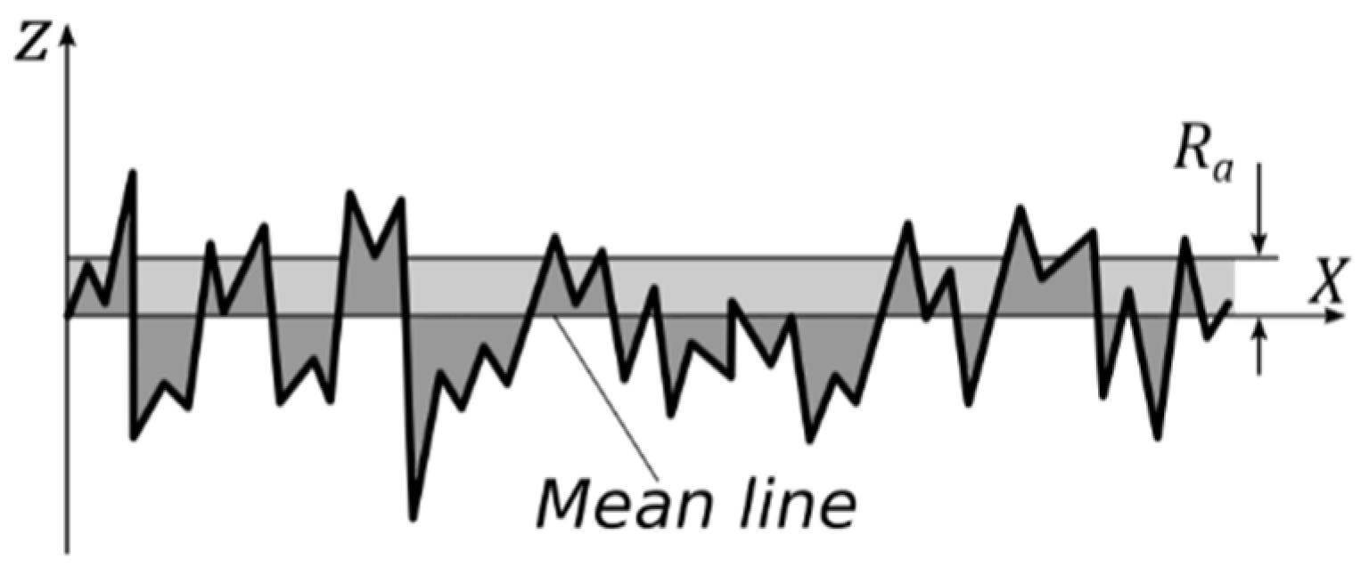
2.1. Surface Roughness Equations
2.2. Governing Equations for Sound Propagation on Solid Surfaces
2.3. Significant Equations for the Principle of Piezoelectric Sensors
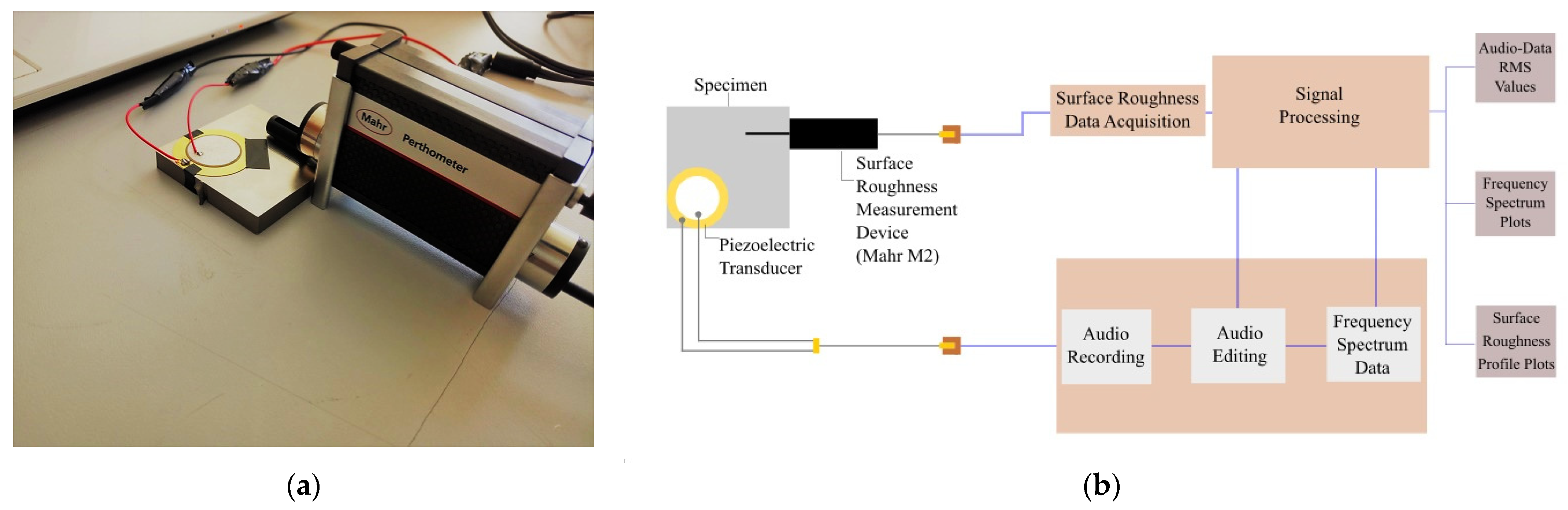
2.4. Experimental Setup
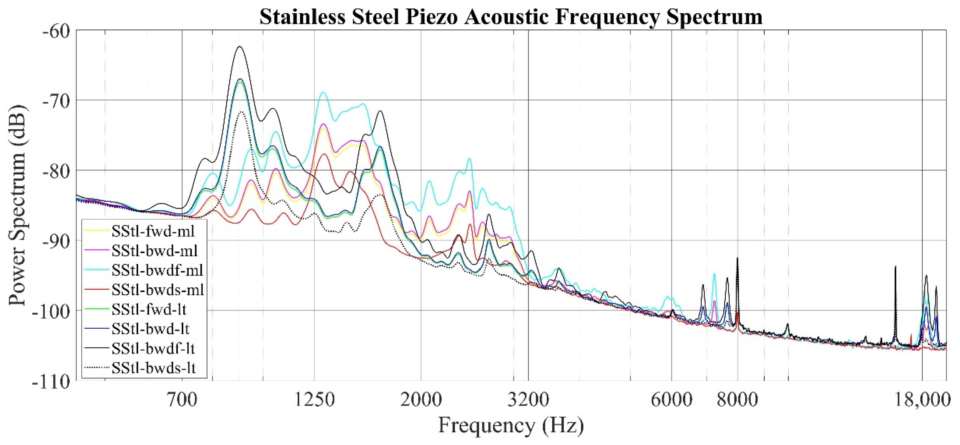
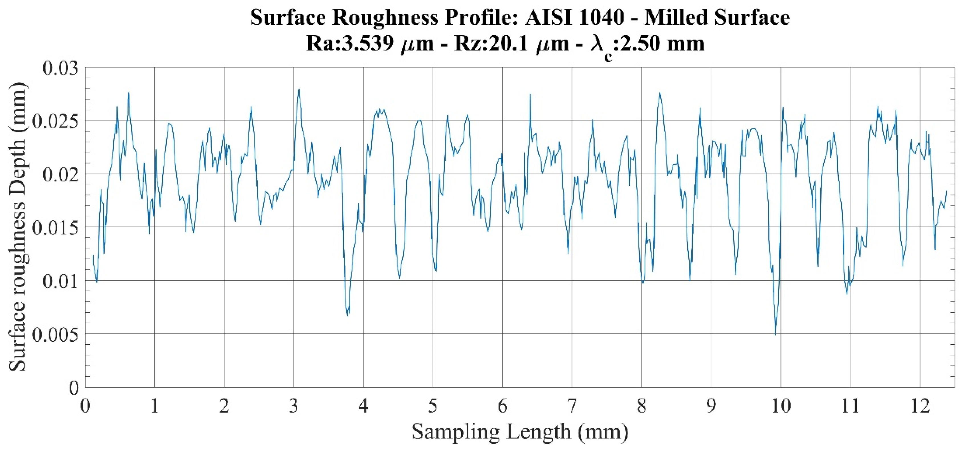
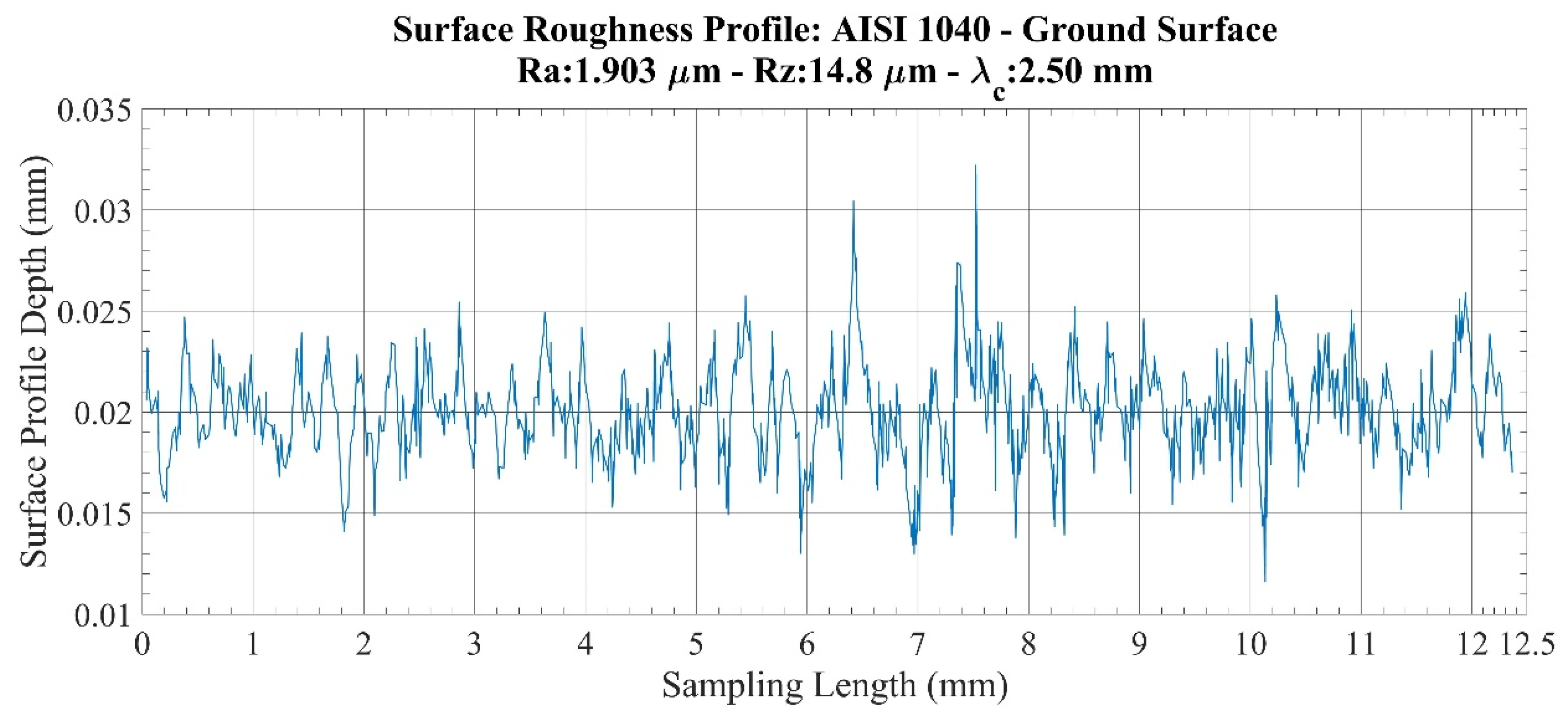
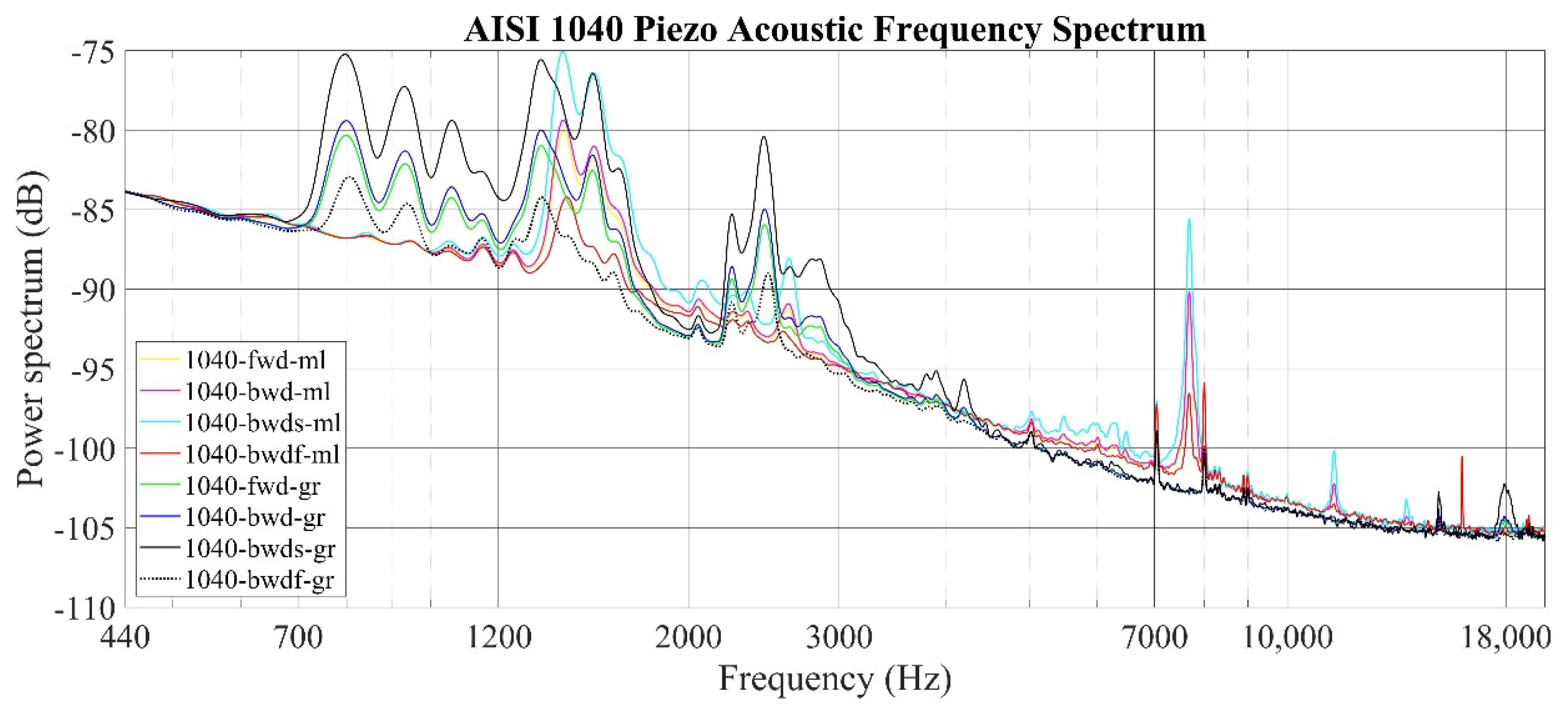
3. Results
4. Discussion
Author Contributions
Funding
Data Availability Statement
Conflicts of Interest
References
- Seifi, R.; Abbasi, K.; Asayesh, M. Effects of contact surface roughness of interference shaft/bush joints on its characteristics. Iran. J. Sci. Technol. Trans. Mech. Eng. 2017, 42, 279–292. [Google Scholar] [CrossRef]
- Yang, G.-M.; Coquille, J.; Fontaine, J.F.; Lambertin, M. Influence of roughness on characteristics of tight interference fit of a shaft and a hub. Int. J. Solids Struct. 2001, 38, 7691–7701. [Google Scholar] [CrossRef]
- Decker, K.-H.; Kabus, K.; Rieg, F.; Hackenschmidt, R.; Engelken, G.; Weidermann, F. Maschinenelemente-Funktion, Gestaltung und Berechnung: Mit 871 Bildern, 164 Berechnungsbeispielen und einem Tabellenband mit 334 Tabellen und Diagrammen. 19; Hanser: München, Germany, 2014. [Google Scholar]
- Steinhilper, W.; Röper, R. Maschinen-und Konstruktionselemente 3: Elastische Elemente, Federn Achsen und Wellen Dichtungstechnik Reibung, Schmierung, Lagerungen; Springer: Berlin/Heidelberg, Germany, 2013. [Google Scholar]
- Bayer, R.; Sirico, J. The influence of surface roughness on wear. Wear 1975, 35, 251–260. [Google Scholar] [CrossRef]
- Svahn, F.; Kassman-Rudolphi, Å.; Wallén, E. The influence of surface roughness on friction and wear of machine element coatings. Wear 2003, 254, 1092–1098. [Google Scholar] [CrossRef]
- Podgornik, B.; Hogmark, S.; Sandberg, O. Influence of surface roughness and coating type on the galling properties of coated forming tool steel. Surf. Coat. Technol. 2004, 184, 338–348. [Google Scholar] [CrossRef]
- Bayoumi, M.R.; Abdellatif, A. Effect of surface finish on fatigue strength. Eng. Fract. Mech. 1995, 51, 861–870. [Google Scholar] [CrossRef]
- Murakami, Y. Metal Fatigue: Effects of Small Defects and Nonmetallic Inclusions; Academic Press: Cambridge, MA, USA, 2019. [Google Scholar]
- Sekercioglu, T.; Gulsoz, A.; Rende, H. The effects of bonding clearance and interference fit on the strength of adhesively bonded cylindrical components. Mater. Des. 2005, 26, 377–381. [Google Scholar] [CrossRef]
- Uehara, K.; Sakurai, M. Bonding strength of adhesives and surface roughness of joined parts. J. Mater. Process. Technol. 2002, 127, 178–181. [Google Scholar] [CrossRef]
- Munson, B.R.; Okiishi, T.H.; Huebsch, W.W.; Rothmayer, A.P. Fluid Mechanics; John Wiley & Sons Singapore: Singapore, 2013. [Google Scholar]
- ISO 21920-2:2021; Geometrical Product Specifications (GPS)—Surface Texture: Profile—Part 2: Terms, Definitions and Surface Texture Parameters. International Organization for Standardization (ISO): Geneva, Switzerland, 2021; p. 78.
- Gadelmawla, E.; Koura, M.M.; Maksoud, T.M.; Elewa, I.M.; Soliman, H. Roughness parameters. J. Mater. Process. Technol. 2002, 123, 133–145. [Google Scholar] [CrossRef]
- Seitavuopio, P.; Rantanen, J.; Yliruusi, J. Use of roughness maps in visualisation of surfaces. Eur. J. Pharm. Biopharm. 2005, 59, 351–358. [Google Scholar] [CrossRef]
- Baldewsing, R. Modulography: Elasticity Imaging of Atherosclerotic Plaques; Erasmus University Rotterdam: Rotterdam, The Netherlands, 2006. [Google Scholar]
- Windecker, R.; Tiziani, H.J. Optical roughness measurements using extended white-light interferometry. Opt. Eng. 1999, 38, 1081–1087. [Google Scholar] [CrossRef]
- Frigieri, E.P.; Campos, P.H.S.; Paiva, A.P.; Balestrassi, P.P.; Ferreira, J.R.; Ynoguti, C.A. A mel-frequency cepstral coefficient-based approach for surface roughness diagnosis in hard turning using acoustic signals and gaussian mixture models. Appl. Acoust. 2016, 113, 230–237. [Google Scholar] [CrossRef]
- Vellekoop, M.J. Acoustic wave sensors and their technology. Ultrasonics 1998, 36, 7–14. [Google Scholar] [CrossRef]
- Tekıner, Z.; Yeşılyurt, S. Investigation of the cutting parameters depending on process sound during turning of AISI 304 austenitic stainless steel. Mater. Des. 2004, 25, 507–513. [Google Scholar] [CrossRef]
- Washabaugh, P.D.; Knauss, W. A reconciliation of dynamic crack velocity and Rayleigh wave speed in isotropic brittle solids. Int. J. Fract. 1994, 65, 97–114. [Google Scholar] [CrossRef]
- Ai, C.S.; Sun, Y.J.; He, G.W.; Ze, X.B.; Li, W.; Mao, K. The milling tool wear monitoring using the acoustic spectrum. Int. J. Adv. Manuf. Technol. 2011, 61, 457–463. [Google Scholar] [CrossRef]
- Downey, J.; O’Leary, P.; Raghavendra, R. Comparison and analysis of audible sound energy emissions during single point machining of HSTS with PVD TiCN cutter insert across full tool life. Wear 2014, 313, 53–62. [Google Scholar] [CrossRef]
- Lu, M.-C.; Wan, B.-S. Study of high-frequency sound signals for tool wear monitoring in micromilling. Int. J. Adv. Manuf. Technol. 2012, 66, 1785–1792. [Google Scholar] [CrossRef]
- Hemmati, F.; Orfali, W.; Gadala, M.S. Roller bearing acoustic signature extraction by wavelet packet transform, applications in fault detection and size estimation. Appl. Acoust. 2016, 104, 101–118. [Google Scholar] [CrossRef]
- Zhao, M.; Lin, J.; Miao, Y.; Xu, X. Detection and recovery of fault impulses via improved harmonic product spectrum and its application in defect size estimation of train bearings. Measurement 2016, 91, 421–439. [Google Scholar] [CrossRef]
- Van Hecke, B.; Yoon, J.; He, D. Low speed bearing fault diagnosis using acoustic emission sensors. Appl. Acoust. 2016, 105, 35–44. [Google Scholar] [CrossRef]
- Lin, W.; Deng, X.H.; Li, X. High sensitive evaluation fatigue of plate using high mode Lamb wave. Appl. Acoust. 2013, 74, 1018–1021. [Google Scholar] [CrossRef]
- Hentati, H.; Kriaa, Y.; Haugou, G.; Chaari, F.; Wali, M.; Zouari, B.; Dammak, F. Influence of elastic wave on crack nucleation—Experimental and computational investigation of brittle fracture. Appl. Acoust. 2017, 128, 45–54. [Google Scholar] [CrossRef]
- Hu, E.; He, Y.; Chen, Y. Experimental study on the surface stress measurement with Rayleigh wave detection technique. Appl. Acoust. 2009, 70, 356–360. [Google Scholar] [CrossRef]
- Castro, B.; Clerice, G.; Ramos, C.; Andreoli, A.; Baptista, F.; Campos, F.; Ulson, J. Partial discharge monitoring in power transformers using low-cost piezoelectric sensors. Sensors 2016, 16, 1266. [Google Scholar] [CrossRef] [Green Version]
- Budoya, D.E.; Baptista, F.G. A comparative study of impedance measurement techniques for structural health monitoring applications. IEEE Trans. Instrum. Meas. 2018, 67, 912–924. [Google Scholar] [CrossRef] [Green Version]
- Aulestia Viera, M.A.; Aguiar, P.R.; Oliveira Junior, P.; Alexandre, F.A.; Lopes, W.N.; Bianchi, E.C.; da Silva, R.B.; D’Addona, D.; Andreoli, A. A time-frequency acoustic emission-based technique to assess workpiece surface quality in ceramic grinding with PZT transducer. Sensors 2019, 19, 3913. [Google Scholar] [CrossRef] [Green Version]
- Viera, M.A.A.; Gotz, R.; de Aguiar, P.R.; Alexandre, F.A.; Fernandez, B.O.; Oliveira Junior, P. A low-cost acoustic emission sensor based on piezoelectric diaphragm. IEEE Sens. J. 2020, 20, 9377–9384. [Google Scholar] [CrossRef]
- Nazarchuk, Z.; Skalskyi, V.; Serhiyenko, O. Propagation of elastic waves in solids. In Acoustic Emission; Springer: Cham, Switzerland, 2017; pp. 29–73. [Google Scholar]
- Rayleigh, L. On waves propagated along the plane surface of an elastic solid. Proc. Lond. Math. Soc. 1885, 1, 4–11. [Google Scholar] [CrossRef]
- Preumont, A. Vibration Control of Active Structures: An Introduction; Springer: Berlin/Heidelberg, Germany, 2018; Volume 246. [Google Scholar]


| Material | ||||
|---|---|---|---|---|
| Longitudinal | Transversal | Surface | ||
| Aluminum | 2.7 | 6.35 | 3.08 | 2.80 |
| Stainless Steel | 8.03 | 5.73 | 3.12 | 2.90 |
| AISI 1040 | 7.80 | 5.92 | 3.28 | 3.01 |
| Aluminum (Milled) | Aluminum (Ground) | Stainless Steel (Milled) | Stainless Steel (Lathed) | AISI 1040 (Milled) | AISI 1040 (Ground) | |
|---|---|---|---|---|---|---|
| Sound RMS | 3.6027 | 1.0279 | 1.2262 | 1.3868 | 0.8783 | 0.8085 |
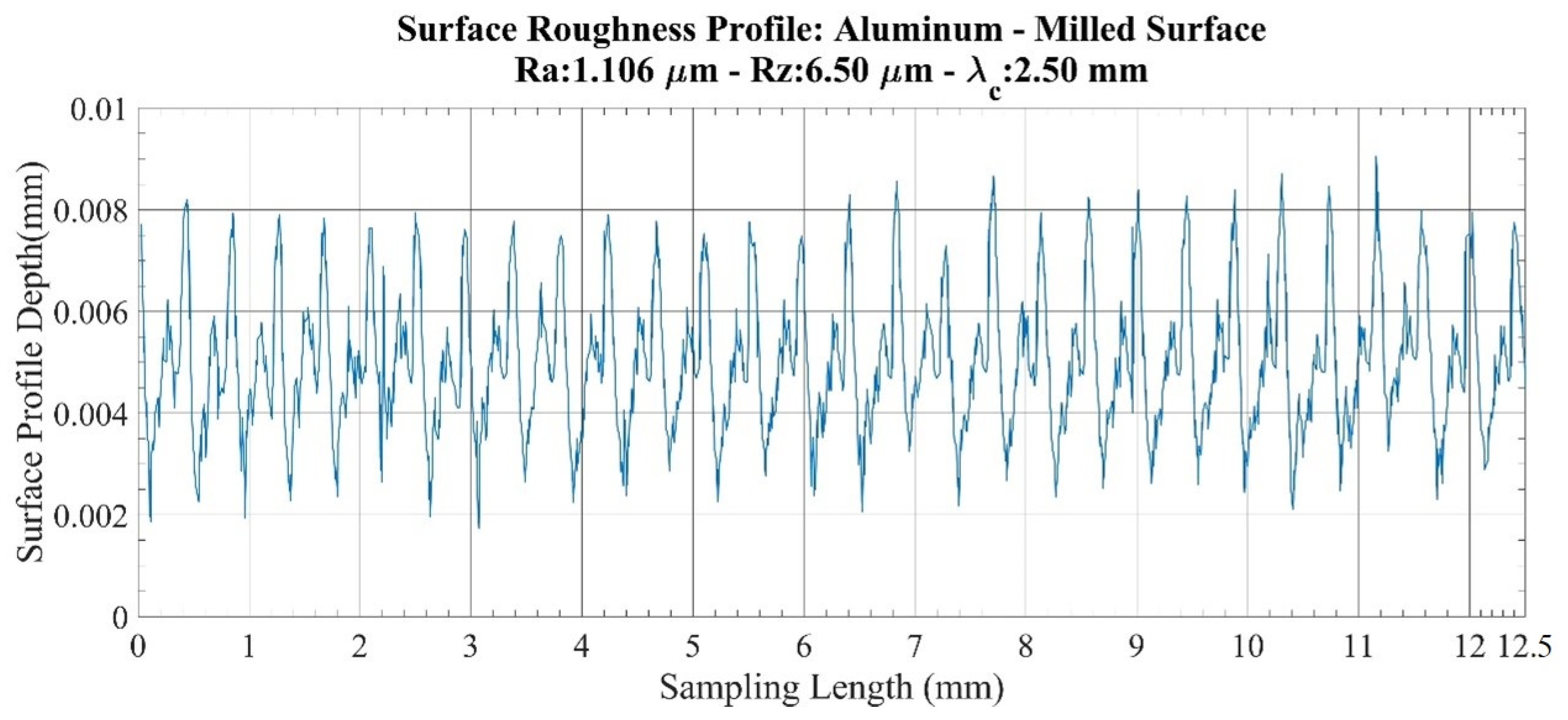
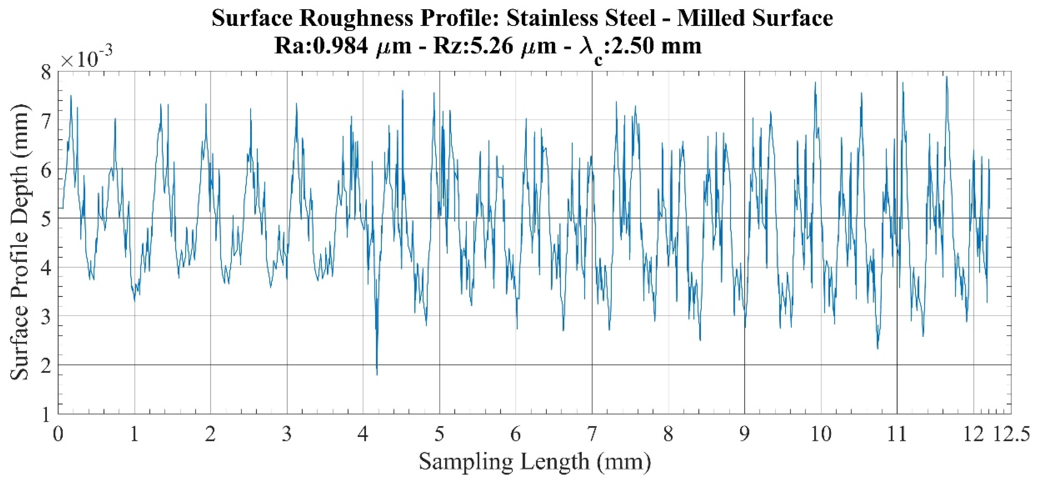
| Ra (μm) | 1.106 | 0.20 | 0.984 | 3.404 | 3.359 | 1.903 |
| Rz (μm) | 6.50 | 2.56 | 5.26 | 14.30 | 20.10 | 14.80 |
| Ars | 28.3730 | 8.0338 | 27.5645 | 33.7739 | 19.8591 | 18.3818 |
| Aps | 11.2109 | 9.4554 | 30.3371 | 39.7898 | 32.8009 | 24.7656 |
| Legend | Specimen | Stroke-Speed | Machining Operation | Sampling Time, Sec |
|---|---|---|---|---|
| Al-fwd-ml | Aluminum | Forward–Standard | Milling | 55 |
| Al-bwd-ml | Aluminum | Backward–Standard | Milling | 48 |
| Al-bwdf-ml | Aluminum | Backward–Fast | Milling | 12.3 |
| Al-bwds-ml | Aluminum | Backward–Slow | Milling | 35.3 |
| Al-fwd-gr | Aluminum | Forward–Standard | Grinding | 55 |
| Al-bwd-gr | Aluminum | Backward–Standard | Grinding | 47.5 |
| Al-bwdf-gr | Aluminum | Backward–Fast | Grinding | 12 |
| Al-bwds-gr | Aluminum | Backward–Slow | Grinding | 35.4 |
| SStl-fwd-ml | Stainless Steel | Forward–Standard | Milling | 56.5 |
| SStl-bwd-ml | Stainless Steel | Backward–Standard | Milling | 48 |
| SStl-bwdf-ml | Stainless Steel | Backward–Fast | Milling | 12.3 |
| SStl-bwds-ml | Stainless Steel | Backward–Slow | Milling | 35.7 |
| SStl-fwd-lt | Stainless Steel | Forward–Standard | Lathing | 52.5 |
| SStl-bwd-lt | Stainless Steel | Backward–Standard | Lathing | 46 |
| SStl-bwdf-lt | Stainless Steel | Backward–Fast | Lathing | 12 |
| SStl-bwds-lt | Stainless Steel | Backward–Slow | Lathing | 34 |
| 1040-fwd-ml | AISI 1040 | Forward–Standard | Milling | 60 |
| 1040-bwd-ml | AISI 1040 | Backward–Standard | Milling | 50 |
| 1040-bwdf-ml | AISI 1040 | Backward–Fast | Milling | 14.5 |
| 1040-bwds-ml | AISI 1040 | Backward–Slow | Milling | 35.5 |
| 1040-fwd-gr | AISI 1040 | Forward–Standard | Grinding | 62 |
| 1040-bwd-gr | AISI 1040 | Backward–Standard | Grinding | 48 |
| 1040-bwdf-gr | AISI 1040 | Backward–Fast | Grinding | 12.5 |
| 1040-bwds-gr | AISI 1040 | Backward–Slow | Grinding | 35.5 |
Publisher’s Note: MDPI stays neutral with regard to jurisdictional claims in published maps and institutional affiliations. |
© 2022 by the authors. Licensee MDPI, Basel, Switzerland. This article is an open access article distributed under the terms and conditions of the Creative Commons Attribution (CC BY) license (https://creativecommons.org/licenses/by/4.0/).
Share and Cite
Kurşun, K.; Güven, F.; Ersoy, H. Utilizing Piezo Acoustic Sensors for the Identification of Surface Roughness and Textures. Sensors 2022, 22, 4381. https://doi.org/10.3390/s22124381
Kurşun K, Güven F, Ersoy H. Utilizing Piezo Acoustic Sensors for the Identification of Surface Roughness and Textures. Sensors. 2022; 22(12):4381. https://doi.org/10.3390/s22124381
Chicago/Turabian StyleKurşun, Kayra, Fatih Güven, and Hakan Ersoy. 2022. "Utilizing Piezo Acoustic Sensors for the Identification of Surface Roughness and Textures" Sensors 22, no. 12: 4381. https://doi.org/10.3390/s22124381
APA StyleKurşun, K., Güven, F., & Ersoy, H. (2022). Utilizing Piezo Acoustic Sensors for the Identification of Surface Roughness and Textures. Sensors, 22(12), 4381. https://doi.org/10.3390/s22124381