
Smart Grid Stability Prediction Model Using Neural Networks to Handle Missing Inputs

 , , , ,
  and
and 
Abstract
:1. Introduction
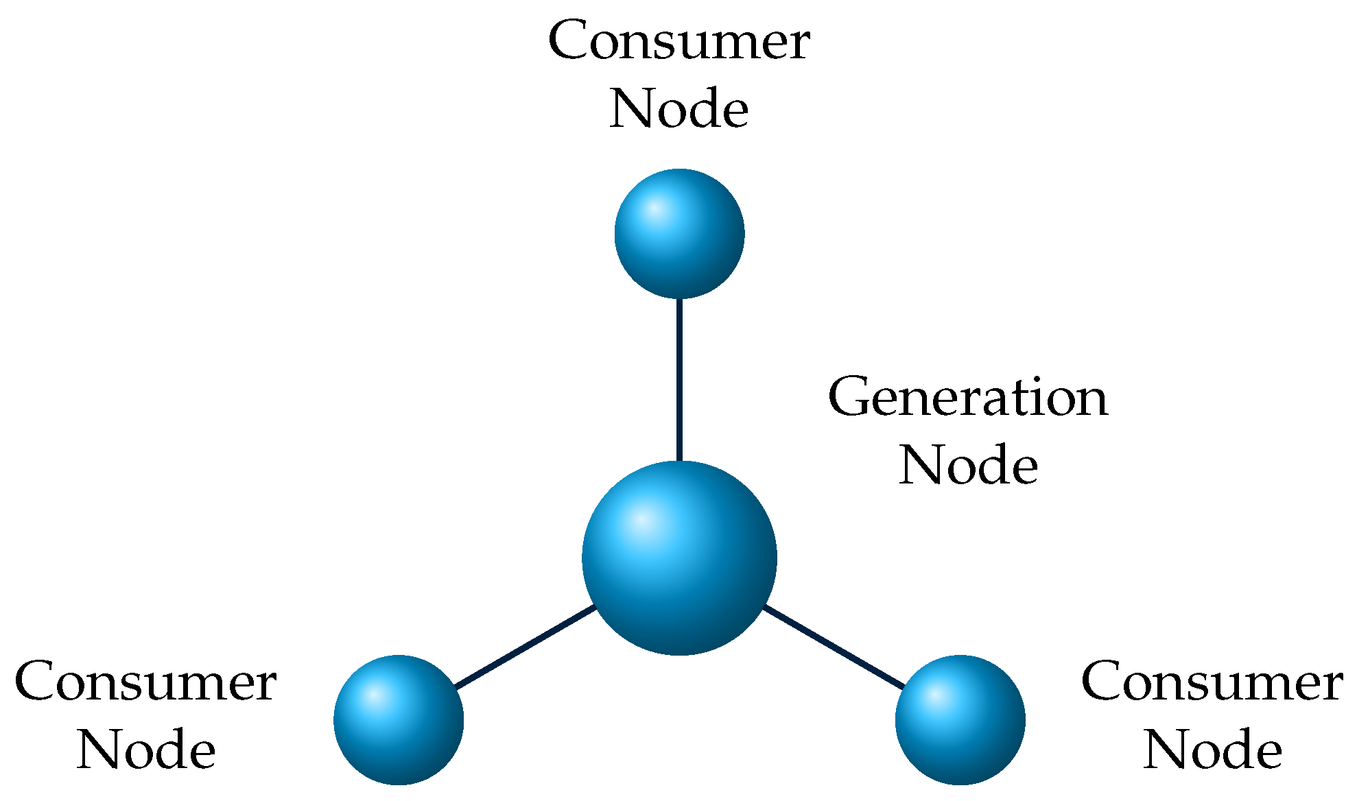
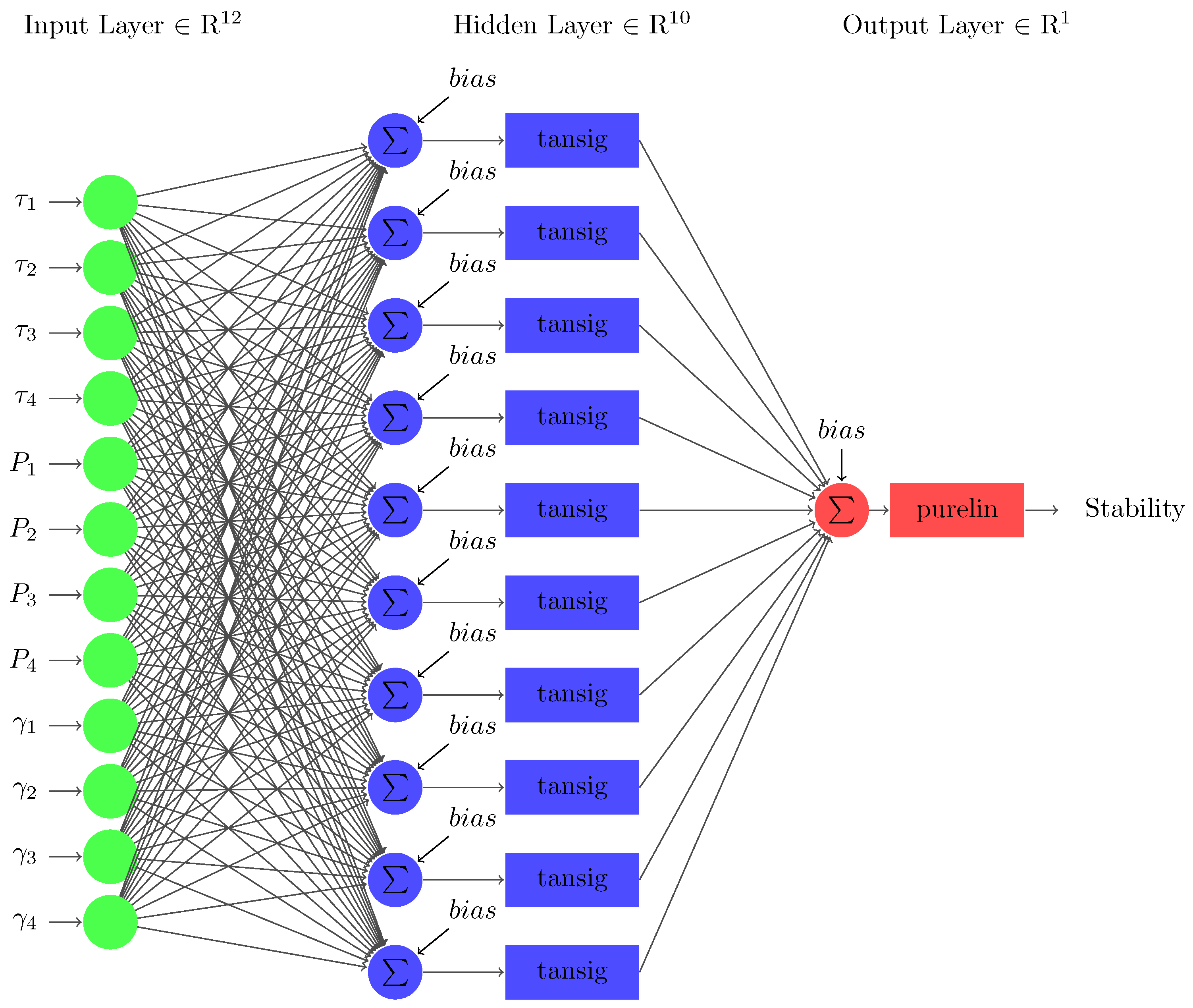
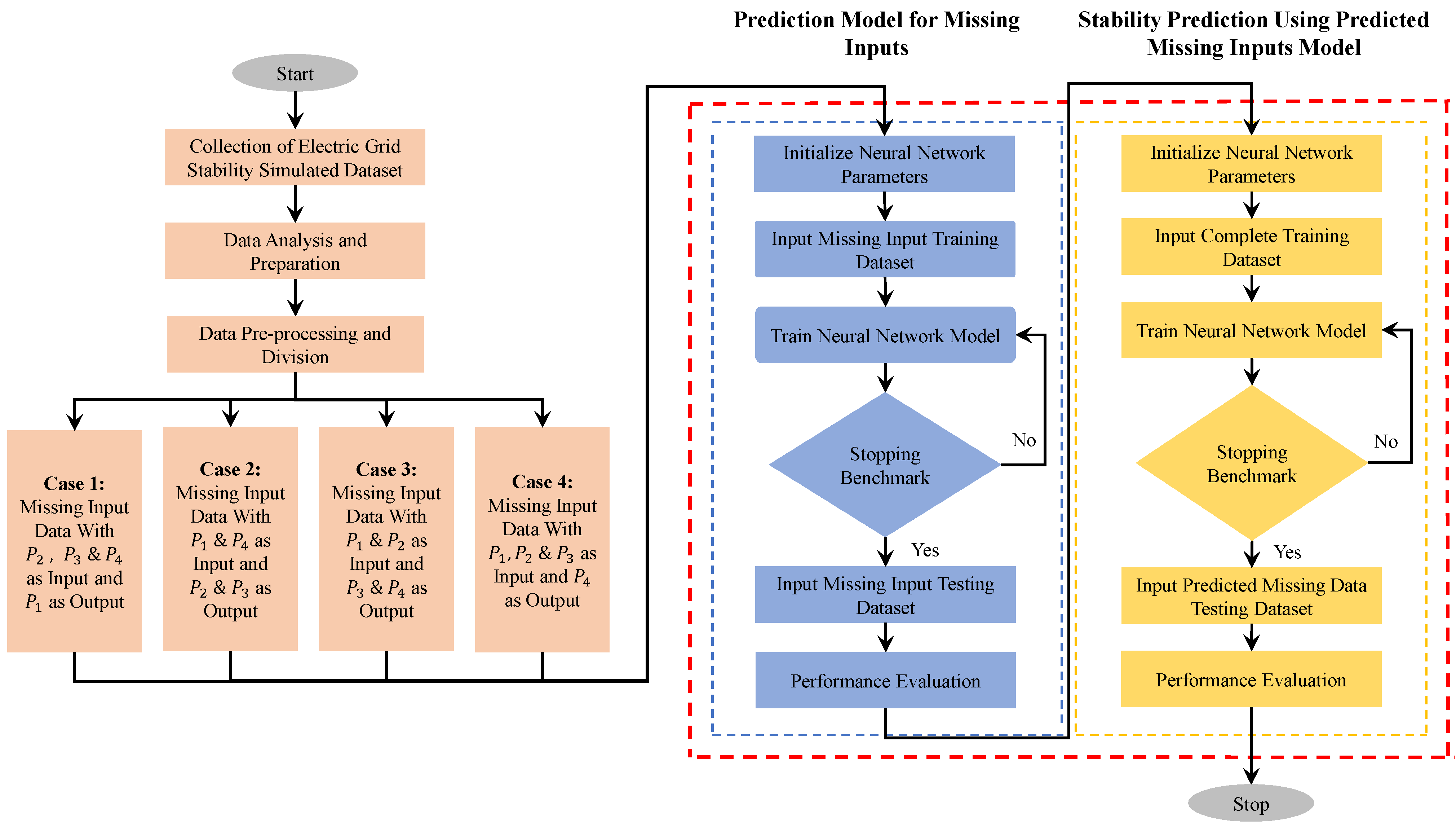
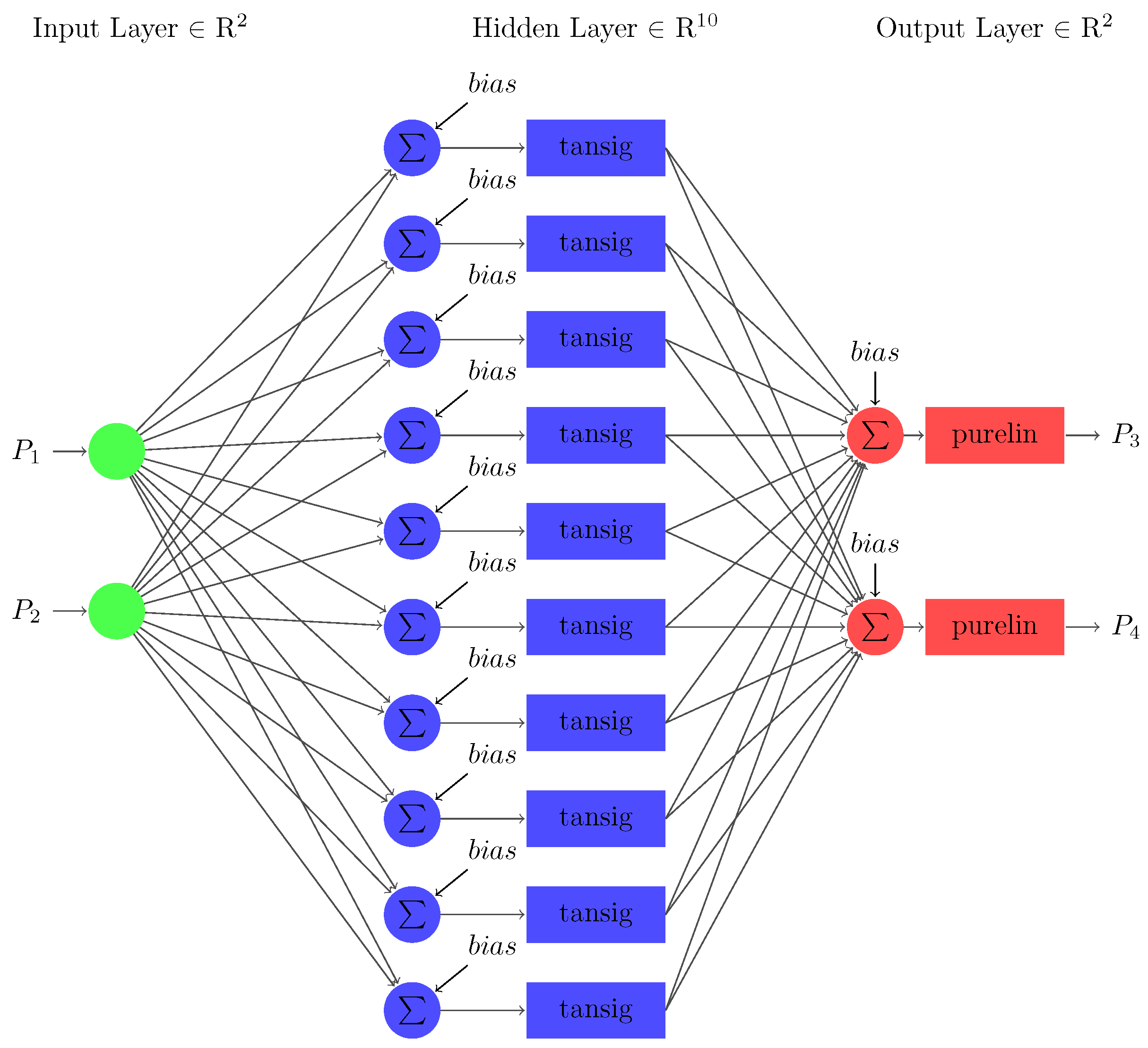
- The classic FFNN is designed to predict the stability of the smart grid system of a four-node star network with complete input data.
- The sub-neural networks are proposed to predict the missing input variables, which are caused due to a sensor, network connection or other system failures. Then, the system’s stability is forecast using these predicted missing input data.
- The performance of the proposed approach is evaluated in four different case studies in which at least one input variable is missing.
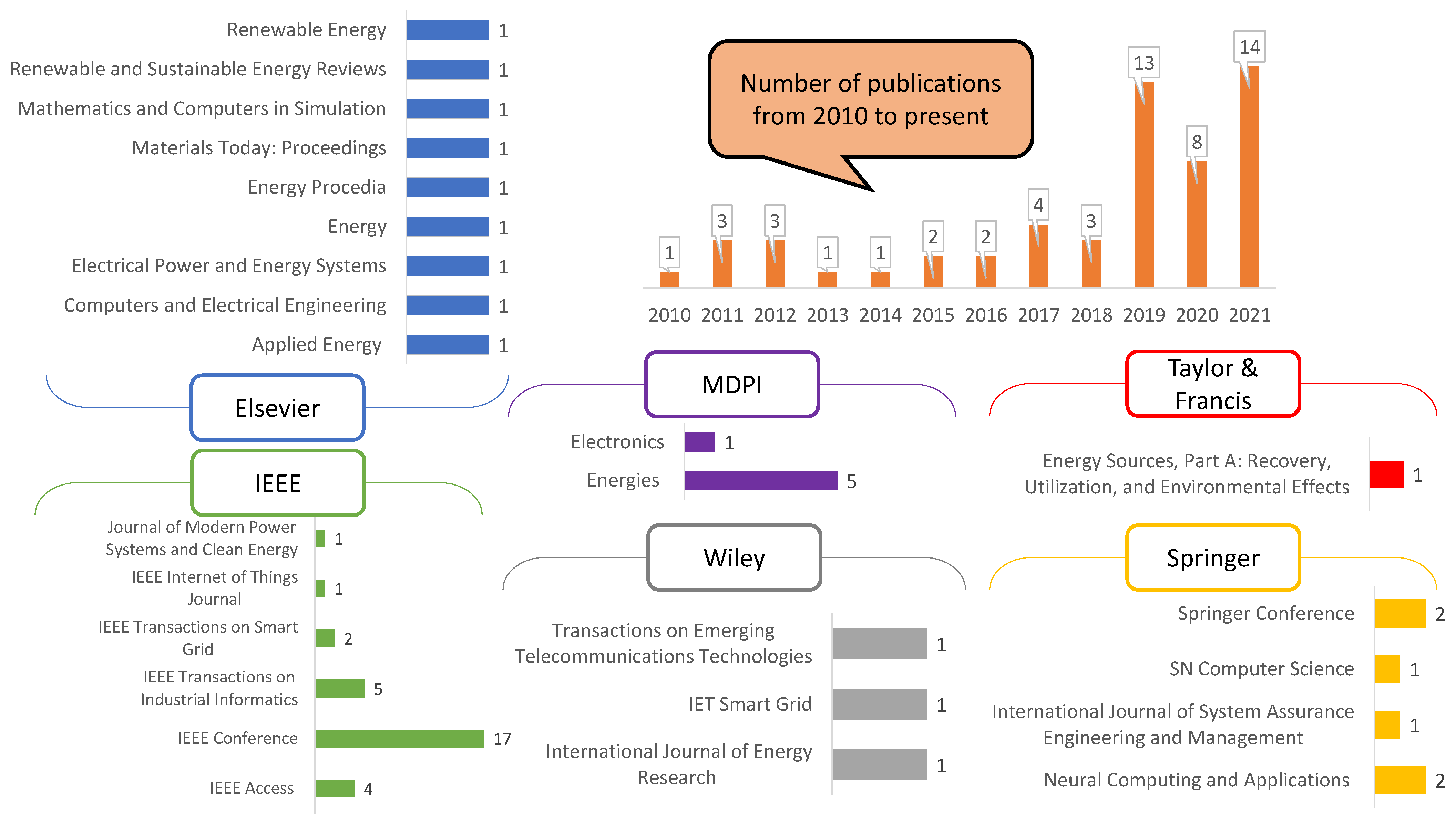
2. Literature Review
- No work was conducted to predict stability when there is a missing parameter. Most studies showed that missing data had been either omitted, unreported or replaced with mean/median values.
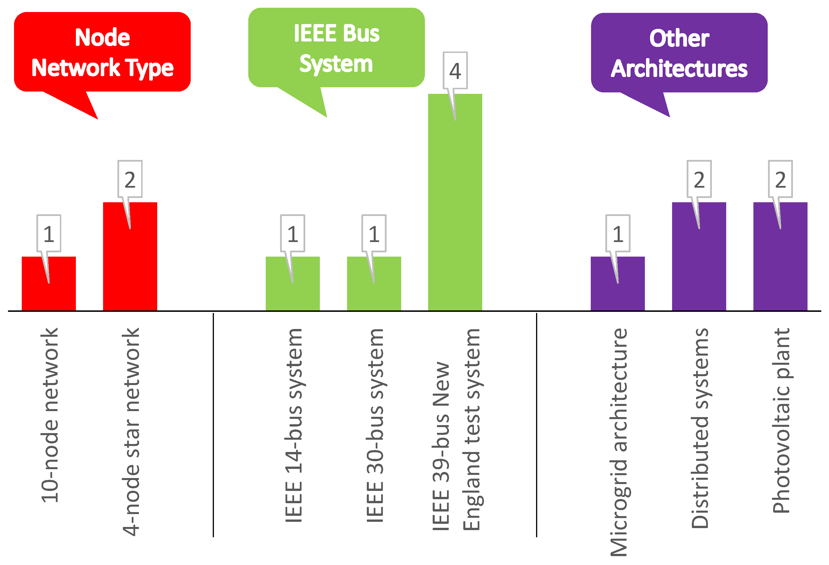
- The most popular architectures used for the case studies are IEEE bus systems and node network types (see Figure 2).
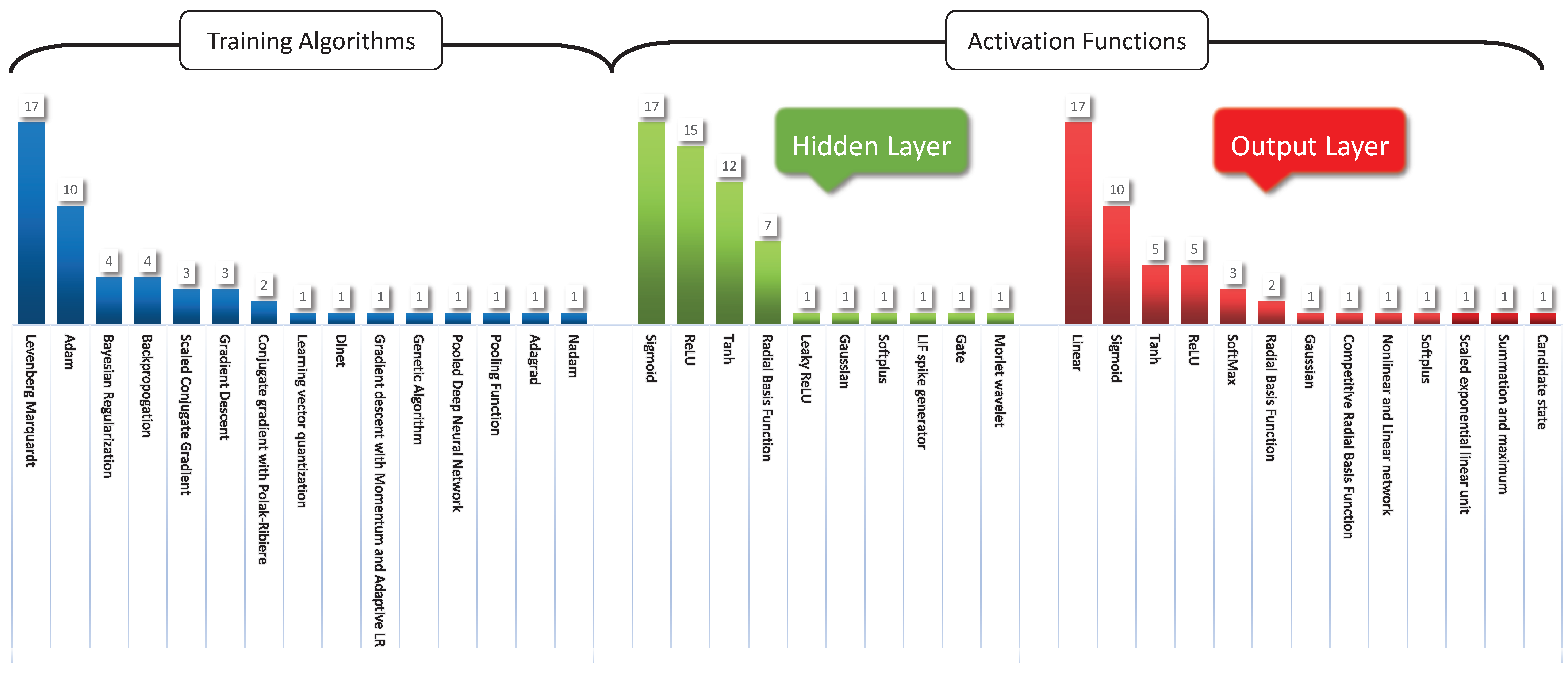
- The Levenberg–Marquardt algorithm is the most frequently used training algorithm for various networks to predict smart grid stability (see Figure 4).
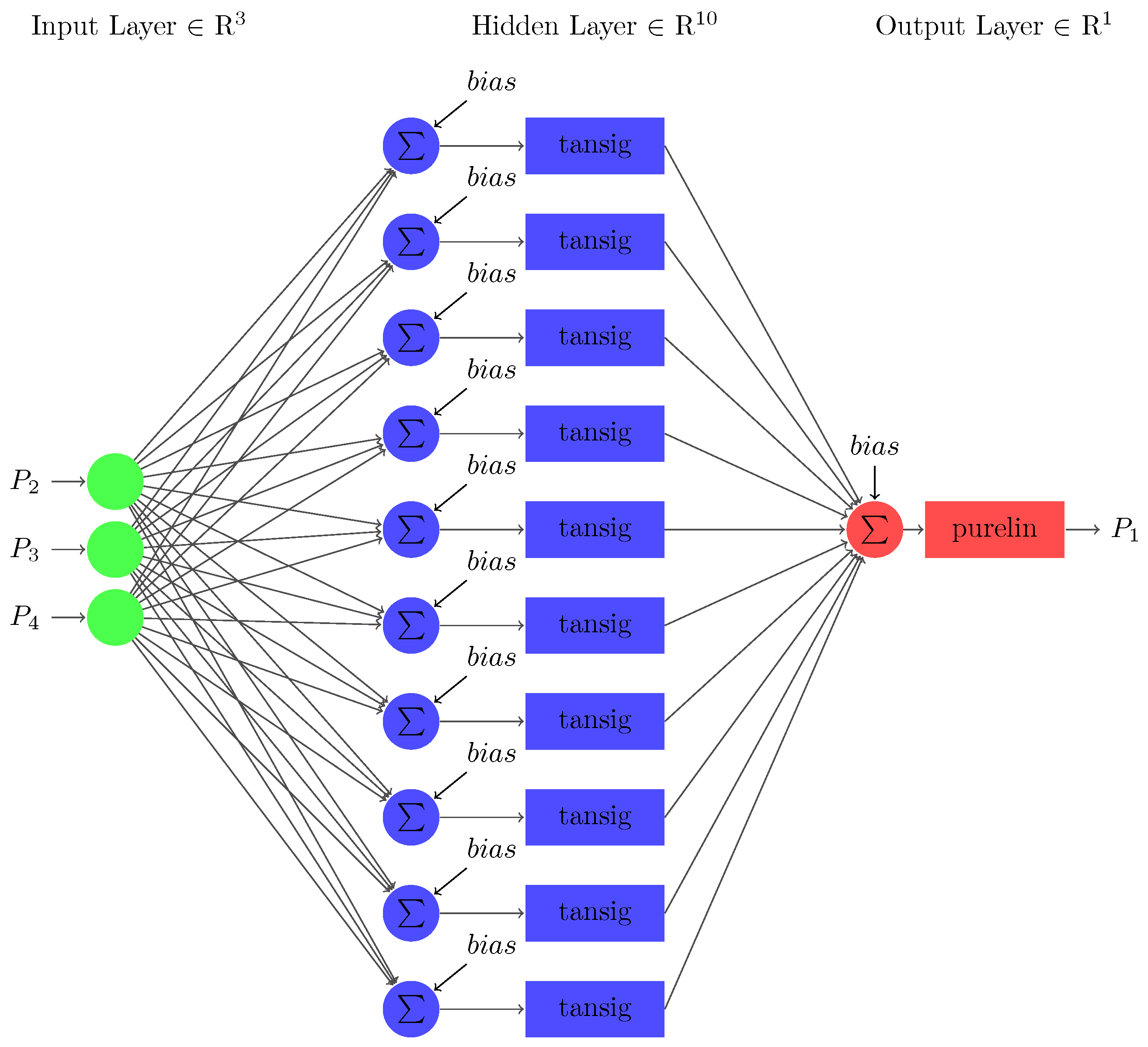
- The tansig and purelin activation functions have frequently been used in various networks’ hidden and output layers to predict smart grid stability (see Figure 4).

| Ref. | Year | Smart Grid Architecture | Neural Network Type | Neural Network Architecture | Activation Functions | Training Algorithm | Performance Measures | Comparison Techniques | |
|---|---|---|---|---|---|---|---|---|---|
| Hidden Layer | Output Layer | ||||||||
| [34] | 2021 | – | FFNN | 2:10:1 | Tanh, Sigmoid | Linear | LM, BR, SCG | MSE, R | RTP, SMP, RTP-SMP, GA, ANN, STW |
| [7] | 2021 | Smart grid with photovoltaic and wind turbine | SSA-RBFNN | – | – | – | – | RMSE | SSA-RBFNN with and without RES |
| [40] | 2021 | – | FFNN | 3:20:1 | Sigmoid | Linear | LM | MSE, RMSE | PV with ANN, Wind with ANN, Hybrid model with ANN |
| [32] | 2021 | – | DNN-RL | – | Leaky ReLU | Leaky ReLU | Adam | MSE | – |
| [29] | 2021 | – | LSTM-RNN | 1:50:50:50:1 | Tanh | Tanh | Adam | MAE, RMSE, MAPE | GBR, SVM |
| [4] | 2021 | four-node star | FFNN | 24:24:12:1 | ReLU | Sigmoid | Adam, GDM, Nadam | Accuracy, Precision, Sensitivity, F-score | CNN, FNN |
| [9] | 2021 | – | GRU-RNN | 3:15:10:1 | Gate | Candidate | AdaGrad | RMSE, MAE | LSSVR, WNN, ELM, SAE, DBN |
| [41] | 2021 | – | SNN | 784:400:400:11 | LIF spike generator | Summation and maximum | – | Precision, Recall, F-score, Accuracy | CNN |
| [8] | 2021 | four-node star | LSTM, BiGRU, ELM | 12:256:128:1, 12:512:256:1, 12:96:30:1 | Sigmoid Softplus | Sigmoid Softplus | Adam | RMSE, MAE, R, PICP, PINC, ACE | BiGRU, LSTM, XGB, LGBM, ANN |
| [42] | 2021 | Distributed systems | DNN-RL | – | ReLU | ReLU | Adam | Peak, Mean, Var, PAR, Cost, Computation time | C-DDPG, DPCS, SWAA |
| [11] | 2021 | – | LSTM, BPNN | 6:96:48:1, 6:48:24:1, 6:10:1 | RBF | Sigmoid | Adam | MAPE, RMSE | LSTM, BPNN, MLSTM, ELM, MLR, SVR |
| [43] | 2021 | – | BPNN | 3:2:3 | Sigmoid | Linear | BP | RMSE | – |
| [14] | 2021 | – | FF-DNN | – | ReLU | SELU | PDNN, Pooling function | FA, MAE, RMSE, SoC, HR | SVM, NN-ARIMA, DBN |
| [44] | 2021 | – | FFNN | – | ReLU | Alpha | BP | Accuracy, Precision, Recall, F-score | PSO-KNN, PSO-NN, PSO-DT, PSO-RF |
| [10] | 2020 | – | CNN-LSTM | – | ReLU | Linear | Adam | RMSE, MAE, NRMSE, F-score | ARIMA, BPNN, SVM, LSTM, CEEMDAN-ARIMA, CEEMDAN-BPNN, CEEMDAN-SVM |
| [45] | 2020 | – | RNN, CNN | – | Sigmoid | Tanh | Adam | Area under the curve, F-score, Precision, Recall, Accuracy | Logistic regression, SVM, LSTM |
| [46] | 2020 | – | NN-LMS | 24:24:24, 24:96:96:4 | ReLU | ReLU | – | – | – |
| [47] | 2020 | – | NARX-RNN | 2:5:1 | Sigmoid | Linear | Conjugate gradient with Polak-Ribiere | NRMSE, RMSE, MAPE | ARMAX |
| [48] | 2020 | – | FFNN | 20:38:1 | Tanh | Linear | Conjugate gradient with Polak-Ribiere | MSE | RTEP, LBPP, IBR without ESS |
| [33] | 2020 | – | IRBDNN | – | – | – | – | RMSE, MAE, MAPE | DNN, ARMA, ELM |
| [30] | 2020 | – | LSTM-RNN | – | Sigmoid, Tanh, ReLU | – | – | Accuracy, Precision, Recall, F-score | GRU, RNN, LSTM |
| [22] | 2020 | IEEE 14-bus system | CNN | – | ReLU | Sigmoid | Adam | Precision, Recall, F-score, Row accuracy | SVM, LGBM, MLP |
| [49] | 2019 | – | FF-BPNN | – | – | – | GA | MSE, Fitness, Accuracy | – |
| [50] | 2019 | – | RNN | Tanh | Sigmoid | BP | MAE, RMSE, MAPE, Pmean | BPNN, SVM, LSTM, RBF | |
| [28] | 2019 | – | CNN-RNN | 100:98:49:1 | ReLU | Softmax | MSE, Recall, PTECC | CNN, CNN-RNN, LSTM | |
| [51] | 2019 | – | ENN | 10:1:1 | – | – | GDM and Adaptive LR, LM | RMSE, NRMSE, MBE, MAE, R, Forecast skill | Similarity search algorithm, ANN, MLP and ARMA, LSTM |
| [12] | 2019 | – | FF-DNN, R-DNN | 2:5:2 | Sigmoid, Tanh, ReLU | Sigmoid, Tanh, ReLU | LM | MAPE | Ensemble Tree Bagger, Generalized linear regression, Shallow neural networks |
| [31] | 2019 | – | CNN, LSTM | 05:10:100 | ReLU | Softmax | – | MCC, F-score, Precision, Recall, Accuracy | Logistic regression, SVM |
| [27] | 2019 | – | ECNN | 32:32:1 | ReLU | Sigmoid, Softmax | Adam | MAE, MAPE, MSE, RMSE | AdaBoost, MLP, RF |
| [23] | 2019 | IEEE 39-bus New England test system | CNN, LSTM | – | Sigmoid | Tanh | GDM | Accuracy | – |
| [52] | 2019 | – | FFNN | 76:20:1, 92:20:1, 92:20:1 | ReLU | Sigmoid | LM | MSE, Accuracy, Precision, Recall, F-score | RF, OneR, JRip, AdaBoost-JRip, SVM and NN (without WOA) |
| [53] | 2019 | – | ECNN | – | – | – | – | MSE, RMSE, MAE, MAPE | |
| [54] | 2019 | – | FF-DNN, R-DNN | – | Sigmoid, Tanh, ReLU | Linear | LM | MAPE, Correlation coefficient, NRMSE | ANN, CNN, CRBM, FF-DNN |
| [25] | 2019 | – | FF-BPNN | – | – | ReLU | GDM | Mean error, MAD, Percent error, MPE, MAPE | Classical forecasting methods |
| [26] | 2019 | – | FF-DNN | 1:5:1, 6:5:1 | Sigmoid | Linear | – | MAPE | DNN-ELM |
| [55] | 2018 | – | FFNN | – | Sigmoid | Nonlinear and linear network | LM | MSE, R | Multilayer ANN Models |
| [56] | 2018 | – | RBF, WRNN | 7:4:3 | RBF | Competitive | LM | Classification accuracy | Pooling Neural Network, LM |
| [13] | 2018 | – | WRNN | 2:16:16:4 | RBF | RBF | – | RMSE | – |
| [57] | 2017 | – | FFNN | 7:96:48:24:1 | Tanh | Gaussian | Dlnet, BP | MAPE | Ten state-of-the-art forecasting methods |
| [58] | 2017 | – | FFNN | 24:5:1 | Sigmoid | Sigmoid | LM | MAPE | AFC-STLF, Bi-level, MI-ANN forecast |
| [59] | 2017 | – | Deep learning based short-term forecasting | 20:30:25:1 | ReLU | ReLU | – | RE | SVM |
| [24] | 2017 | 10-node network | FFNN, WNN-LQE | 8:10:1 | Morlet wavelet | Sigmoid | – | SNR | LQE-based WNN, BPNN, ARIMA, Kalman, XCoPred algorithms |
| [60] | 2016 | – | FFNN | 3:20:10:3 | Sigmoid | Linear | LM, BR | MSE, R | LM, BR |
| [15] | 2016 | – | FFNN | 8:10:1 | Sigmoid | Linear | – | MAE, MAPE, RMSE, R, MSE | GA-MdBP, CGA-MdBP, CGASA-MdBP |
| [16] | 2015 | IEEE 30-bus system | FFNN | 4:10:1 | RBF | – | SCG supervised learning | MSE, PDF, CDF | – |
| [61] | 2015 | – | FFNN | 10:1:20 | Tanh | Tanh | LVQ | Mean Error, Maximum Error, Success % | – |
| [62] | 2014 | – | FFNN | 7:(10-15):1 | Sigmoid | Linear | LM | R, MAPE | – |
| [17] | 2013 | – | FFNN | – | – | – | LM | MER, MAE, MAPE | – |
| [63] | 2012 | Microgrid architecture: residential smart house aggregator | BPNN | 10:1:1 | Tanh | Linear | LM, SCG | Solar insulation and air temperature | – |
| [64] | 2012 | IEEE 39-bus New England test system | FF-BPNN | 20:10:5:1 | Tanh | Sigmoid | LM, BR | Stability | – |
| [6] | 2012 | IEEE 39-bus New England test system | RBF | 30:30:9, 30:30:10 | RBF | Linear | LM | Training Time, Testing Time, Number of misses, MSE, Classification accuracy % | |
| [18] | 2011 | IEEE 39-bus New England test system | RBF | 36:36:1 | Gaussian | Linear | Training time, Testing time, Number of misses, MSE, False alarms %, Misses %, Classification accuracy % | Traditional NR method | |
| [65] | 2011 | Grid-connected PV plant | BPNN | 16:15:7:1 | Sigmoid | Linear | LM | MABE, RMSE, R | – |
| [66] | 2011 | Medium tension distribution system | RBF | 33:119:33, 33:129:33 | RBF | Linear | – | MSE, SPREAD | – |
| [67] | 2010 | – | BPNN, FFNN | 8:8:30:1 | Tanh | Linear | LM, BR | MSE | LM, BR, OSS |
3. Mathematical Modeling and Data Description of Four-Node Star Network
3.1. Mathematical Modeling and Stability Analysis of Four-Node Star Network
3.1.1. Mathematical Modeling
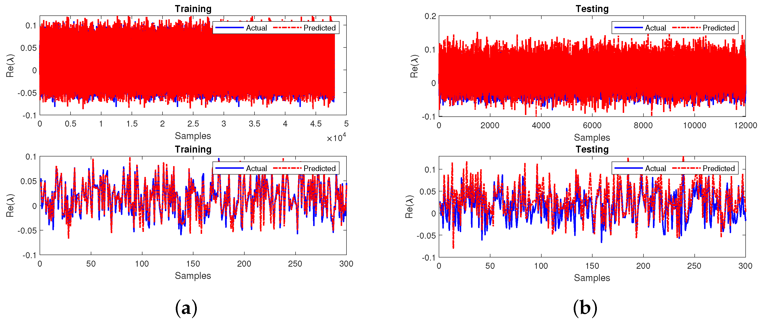
3.1.2. Stability Analysis
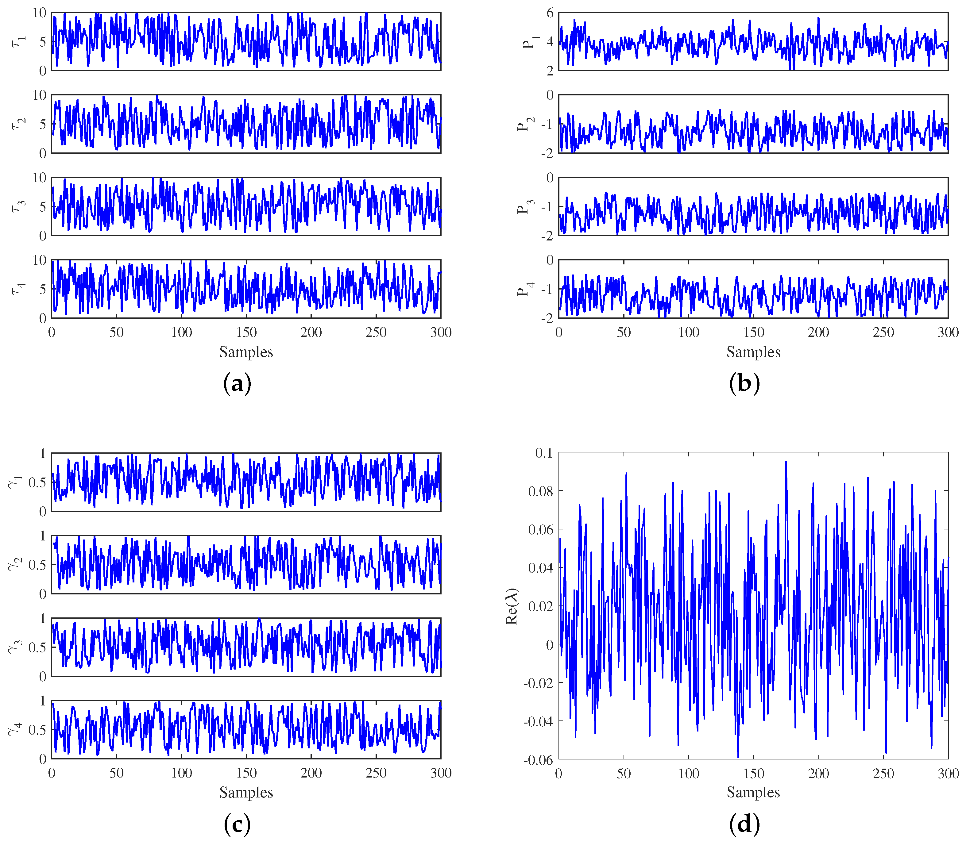
3.2. Data Description of Four-Node Star Network
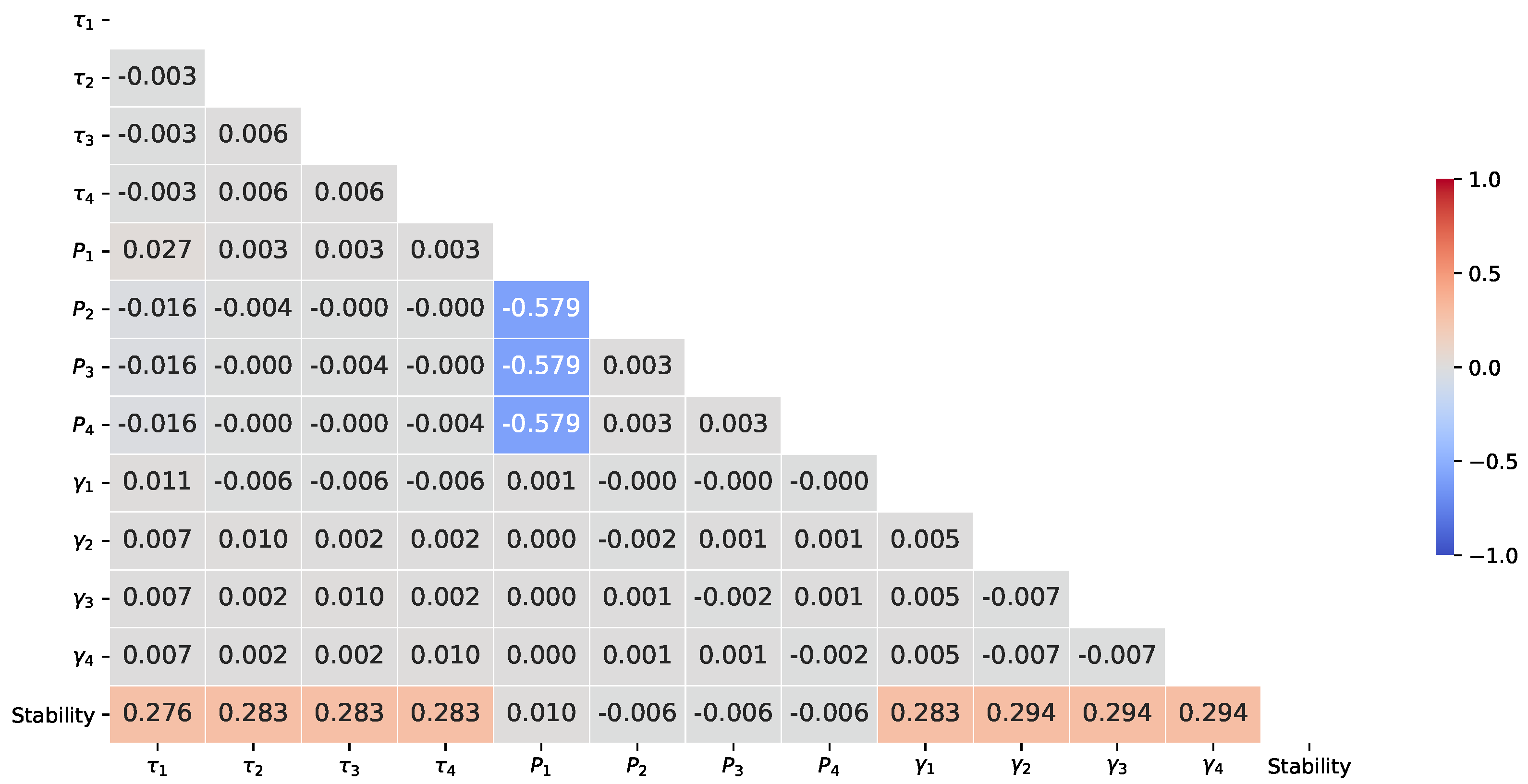
3.3. Correlation Analysis
4. Development and Performance Evaluation of Feedforward Neural Network
5. Development and Performance Evaluation of Feedforward Neural Network to Handle Missing Input
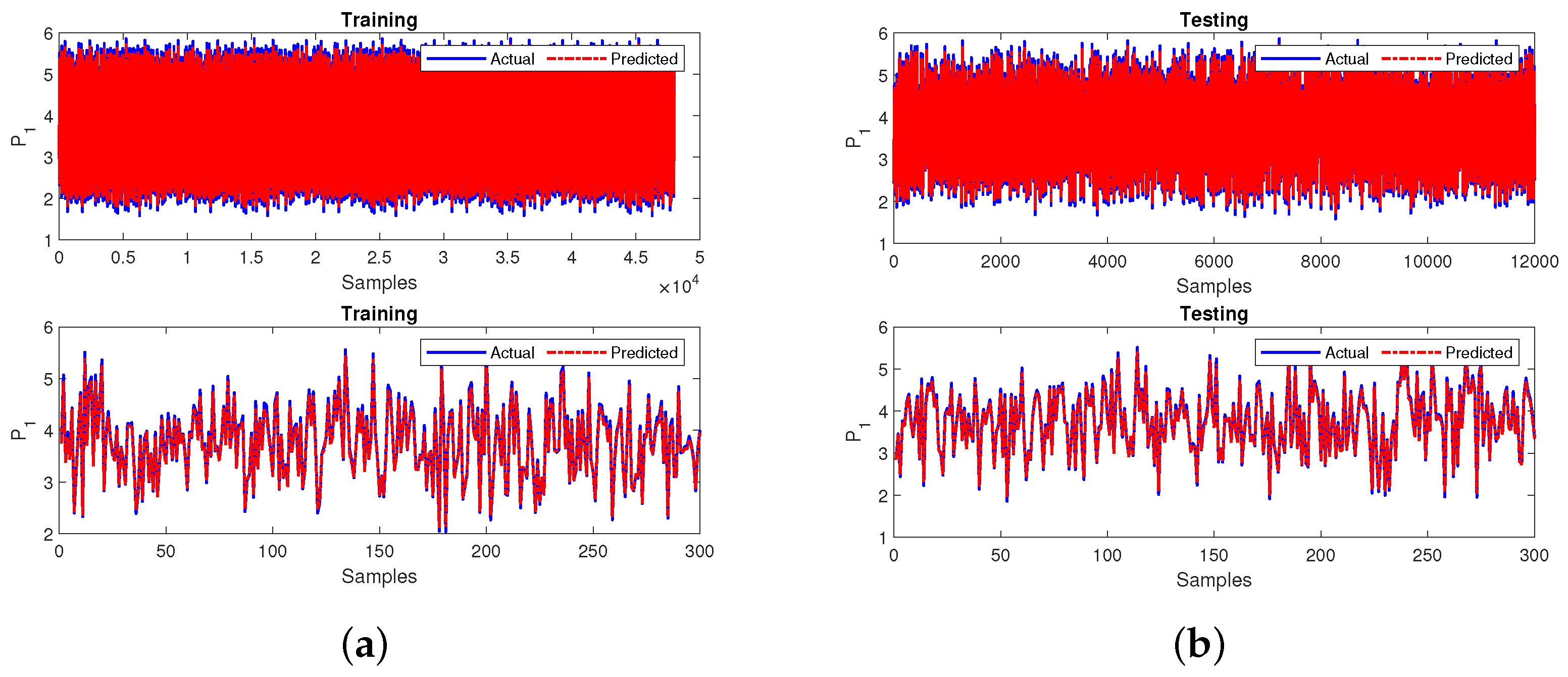
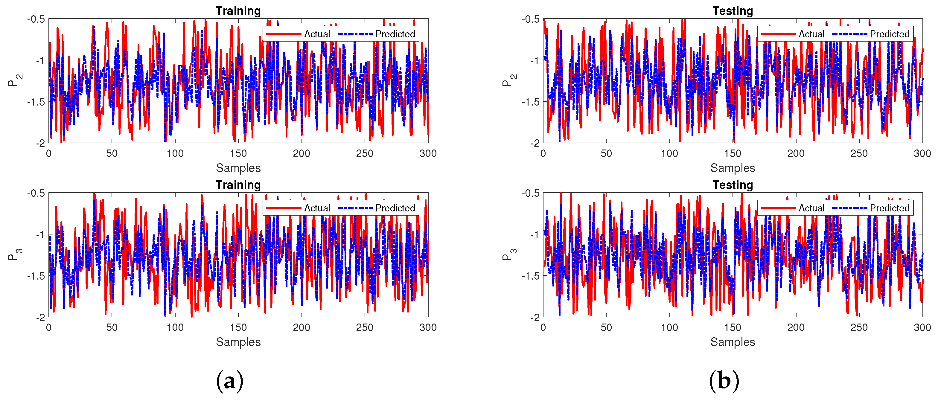
5.1. Case 1
5.2. Case 2
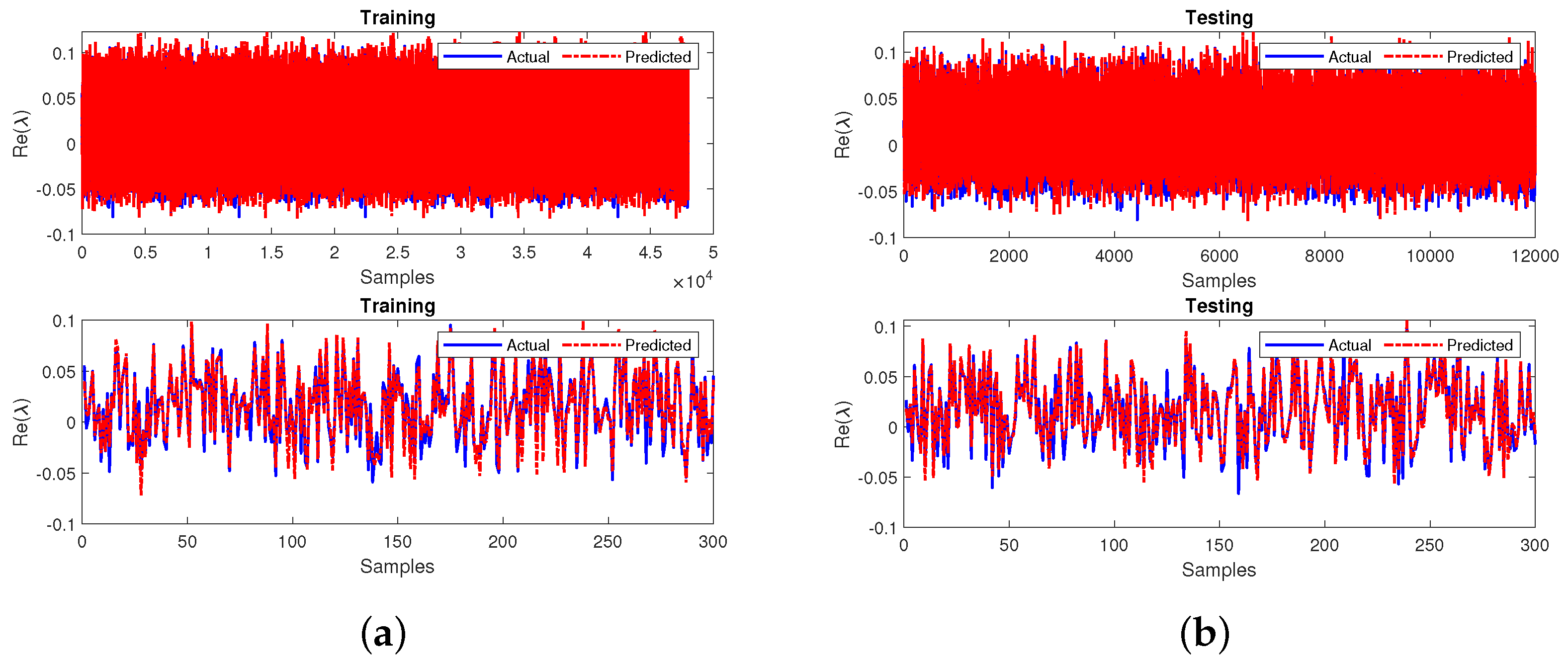
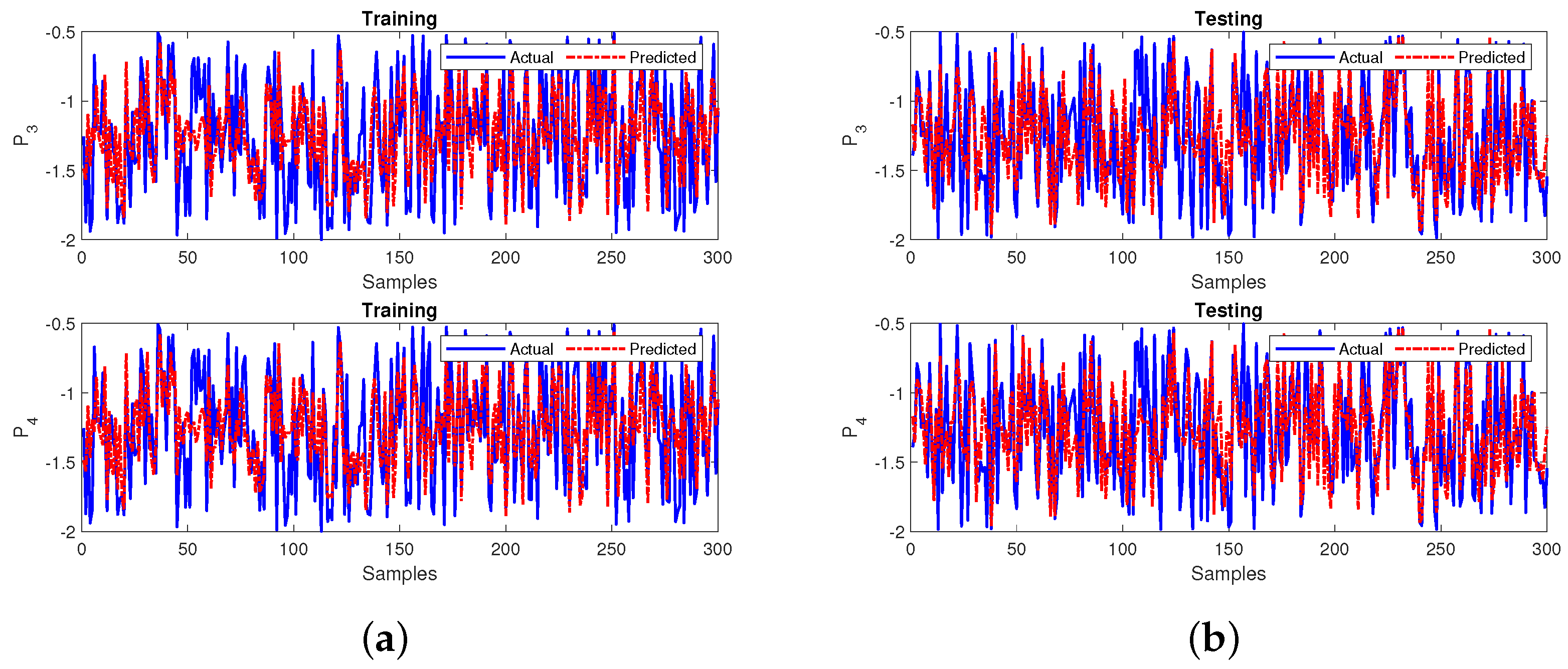
5.3. Case 3
5.4. Case 4
5.5. Summary
6. Conclusions
Author Contributions
Funding
Institutional Review Board Statement
Informed Consent Statement
Data Availability Statement
Conflicts of Interest
Abbreviations
| AdaBoost | Adaptive Boosting |
| AdaGrad | Adaptive Gradient algorithm |
| Adam | Adaptive Movement Estimation |
| ACE | Average Coverage Error |
| Adaptive LR | Adaptive Linear Regression |
| AFC | Accurate and Fast Converging |
| ANN | Artificial Neural Network |
| ARIMA | Autoregressive Integrated Moving Average |
| ARMA | Autoregressive Moving Average |
| ARMAX | Autoregressive-Moving-Average Model With Exogenous Inputs |
| BiGRU | Bidirectional Gated Recurrent Unit |
| BP | Back Propagation |
| BPNN | Back Propagation Neural Network |
| BR | Bayesian Regularization |
| C-DDPG | Centralized Based Deep Deterministic Policy Gradient |
| CDF | Cumulative Distribution Function |
| CEEMDAN | Complete Ensemble Empirical Mode Decomposition Adaptive Noise |
| CGA | Chaos Search Genetic Algorithm |
| CGASA | Chaos Search Genetic Algorithm Furthermore, Simulated Annealing |
| CNN | Convolutional Neural Network |
| CRBM | Convolutional Restricted Boltzmann Machine |
| DBN | Deep Belief Network |
| DNN | Deep Neural Network |
| DPCS | Distributed Power Consumption Scheduling |
| DSGC | Decentral Smart Grid Control |
| DT | Decision Tree |
| ECNN | Enhanced Convolutional Neural Network |
| ELM | Extreme Learning Machine |
| ENN | Elman Neural Network |
| ESS | Energy Storage Systems |
| FA | Forecast Accuracy |
| FF | Feedforward |
| FFNN | Feedforward Neural Network |
| FS | Forecast Skill |
| GA | Genetic Algorithm |
| GBR | Gradient Boosting Regression |
| GDM | Gradient Descent Method |
| GRU | Gated Recurrent Unit |
| HR | Hit Rate |
| IBR | Inclining Block Rate |
| IRBDNN | Iterative Resblock Based Deep Neural Network |
| KNN | k-Nearest Neighbors |
| LBPP | Load Based Pricing Policy |
| LGBM | Light Gradient Boosting Machine |
| LIF | Leaky Integrate and Fire Neuron |
| LM | Levenberg–Marquardt |
| LMS | Lagrange Multiplier Selection |
| LQE | Link Quality Estimation |
| LSSVR | Least Squares Support Vector Regression |
| LVQ | Learning Vector Quantization |
| MABE | Mean Absolute Bias Error |
| MAD | Median Absolute Deviation |
| MAE | Mean Absolute Error |
| MAPE | Mean Absolute Percentage Error |
| MBE | Mean Biased Error |
| MCC | Matthews Correlation Coefficient |
| MdBP | Modified Back Propagation |
| MER | Mean Error Rate |
| MI-ANN | Mutual Information Artificial Neural Network |
| MLP | Multi-Layer Perceptron |
| MLR | Multi-variable Linear Regression |
| MLSTM | Multiplicative Long Short-Term Memory |
| MNE | Mean Normalized Error |
| MPE | Mean Percentage Error |
| MSE | Mean Square Error |
| Nadam | Nesterov-accelerated Adaptive Moment Estimation |
| NARX | Nonlinear Autoregressive Network With Exogenous Inputs |
| NN | Neural Network |
| NRMSE | Normalized Root Mean Square Error |
| PAR | Peak To Average Ratio |
| Probability Density Function | |
| PDNN | Pooling Based Deep Neural Network |
| PICP | Prediction Interval Coverage Probability |
| PINC | Prediction Interval Nominal Confidence |
| PSO | Particle Swarm Optimization |
| PTECC | Proportion Of Total Energy Classified Correctly |
| PV | Photo Voltaic |
| R | Correlation Coefficient |
| RBF | Radial Basis Function |
| RBFNN | Based Radial Basis Function |
| RDNN | Recurrent Deep Neural Network |
| RE | Relative Error |
| ReLU | Rectified Linear Activation Unit |
| RES | Renewable Energy Sources |
| RF | Random Forest |
| RL | Reinforcement Learning |
| RMSE | Root Mean Square Error |
| RNN | Recurrent Neural Network |
| RTEP | Real Time Electrical Pricing |
| RTP | Real Time Price |
| SAE | Sparse Auto Encoder |
| SCG | Scaled Conjugate Gradient |
| SMP | Spot Market Price |
| SNN | Spiking Neural Network |
| SNR | Signal to Noise Ratio |
| SoC | Speed of Convergence |
| SPREAD | Spread of Radial Basis Functions |
| SSA | Salp Swam Algorithm |
| STLF | Short Term Load Forecasting |
| STW | Sliding Time Window |
| SVM | Support Vector Machine |
| SWAA | Sample Weighted Average Approximation |
| Tanh | Hyperbolic Tangent Function |
| WNN | Wavelet Neural Network |
| WOA | Whale Optimization Algorithm |
| WRNN | Wavelet Recurrent Neural Network |
| XGB | Extreme Gradient Boosting |
References
- Gharavi, H.; Ghafurian, R. Smart Grid: The Electric Energy System of the Future; IEEE: Piscataway, NJ, USA, 2011; Volume 99. [Google Scholar]
- McLaughlin, K.; Friedberg, I.; Kang, B.; Maynard, P.; Sezer, S.; McWilliams, G. Secure communications in smart grid: Networking and protocols. In Smart Grid Security; Elsevier: Amsterdam, The Netherlands, 2015; pp. 113–148. [Google Scholar]
- Rathnayaka, A.D.; Potdar, V.M.; Dillon, T.; Kuruppu, S. Framework to manage multiple goals in community-based energy sharing network in smart grid. Int. J. Electr. Power Energy Syst. 2015, 73, 615–624. [Google Scholar] [CrossRef]
- Breviglieri, P.; Erdem, T.; Eken, S. Predicting Smart Grid Stability with Optimized Deep Models. SN Comput. Sci. 2021, 2, 1–12. [Google Scholar] [CrossRef]
- Schäfer, B.; Grabow, C.; Auer, S.; Kurths, J.; Witthaut, D.; Timme, M. Taming instabilities in power grid networks by decentralized control. Eur. Phys. J. Spec. Top. 2016, 225, 569–582. [Google Scholar] [CrossRef]
- Verma, K.; Niazi, K. Generator coherency determination in a smart grid using artificial neural network. In Proceedings of the 2012 IEEE Power and Energy Society General Meeting, San Diego, CA, USA, 22–26 July 2012; pp. 1–7. [Google Scholar]
- Karthikumar, K.; Karthik, K.; Karunanithi, K.; Chandrasekar, P.; Sathyanathan, P.; Prakash, S.V.J. SSA-RBFNN strategy for optimum framework for energy management in Grid-Connected smart grid infrastructure modeling. Mater. Today Proc. 2021. [Google Scholar] [CrossRef]
- Massaoudi, M.; Abu-Rub, H.; Refaat, S.S.; Chihi, I.; Oueslati, F.S. Accurate Smart-Grid Stability Forecasting Based on Deep Learning: Point and Interval Estimation Method. In Proceedings of the 2021 IEEE Kansas Power and Energy Conference (KPEC), Manhattan, KS, USA, 19–20 April 2021; pp. 1–6. [Google Scholar]
- Xia, M.; Shao, H.; Ma, X.; de Silva, C.W. A Stacked GRU-RNN-based Approach for Predicting Renewable Energy and Electricity Load for Smart Grid Operation. IEEE Trans. Ind. Inform. 2021, 17, 7050–7059. [Google Scholar] [CrossRef]
- Gao, B.; Huang, X.; Shi, J.; Tai, Y.; Zhang, J. Hourly forecasting of solar irradiance based on CEEMDAN and multi-strategy CNN-LSTM neural networks. Renew. Energy 2020, 162, 1665–1683. [Google Scholar] [CrossRef]
- Li, J.; Deng, D.; Zhao, J.; Cai, D.; Hu, W.; Zhang, M.; Huang, Q. A novel hybrid short-term load forecasting method of smart grid using mlr and lstm neural network. IEEE Trans. Ind. Inform. 2021, 17, 2443–2452. [Google Scholar] [CrossRef]
- Mohammad, F.; Kim, Y.C. Energy load forecasting model based on deep neural networks for smart grids. Int. J. Syst. Assur. Eng. Manag. 2020, 11, 824–834. [Google Scholar] [CrossRef]
- Capizzi, G.; Sciuto, G.L.; Napoli, C.; Tramontana, E. Advanced and adaptive dispatch for smart grids by means of predictive models. IEEE Trans. Smart Grid 2018, 9, 6684–6691. [Google Scholar] [CrossRef]
- Jeyaraj, P.R.; Nadar, E.R.S. Computer-assisted demand-side energy management in residential smart grid employing novel pooling deep learning algorithm. Int. J. Energy Res. 2021, 45, 7961–7973. [Google Scholar] [CrossRef]
- Islam, B.; Baharudin, Z.; Nallagownden, P. Development of chaotically improved meta-heuristics and modified BP neural network-based model for electrical energy demand prediction in smart grid. Neural Comput. Appl. 2017, 28, 877–891. [Google Scholar] [CrossRef]
- Gupta, S.; Kazi, F.; Wagh, S.; Kambli, R. Neural network based early warning system for an emerging blackout in smart grid power networks. In Intelligent Distributed Computing; Springer: Berlin/Heidelberg, Germany, 2015; pp. 173–183. [Google Scholar]
- Neupane, B.; Perera, K.S.; Aung, Z.; Woon, W.L. Artificial neural network-based electricity price forecasting for smart grid deployment. In Proceedings of the 2012 International Conference on Computer Systems and Industrial Informatics, Sharjah, United Arab Emirates, 18–20 December 2012; pp. 1–6. [Google Scholar]
- Verma, K.; Niazi, K. Determination of vulnerable machines for online transient security assessment in smart grid using artificial neural network. In Proceedings of the 2011 Annual IEEE India Conference, Yderabad, India, 16–18 December 2011; pp. 1–5. [Google Scholar]
- Sakellariou, M.; Ferentinou, M. A study of slope stability prediction using neural networks. Geotech. Geol. Eng. 2005, 23, 419–445. [Google Scholar] [CrossRef]
- Tu, J.V. Advantages and disadvantages of using artificial neural networks versus logistic regression for predicting medical outcomes. J. Clin. Epidemiol. 1996, 49, 1225–1231. [Google Scholar] [CrossRef]
- Nijman, S.; Leeuwenberg, A.; Beekers, I.; Verkouter, I.; Jacobs, J.; Bots, M.; Asselbergs, F.; Moons, K.; Debray, T. Missing data is poorly handled and reported in prediction model studies using machine learning: A literature review. J. Clin. Epidemiol. 2022, 142, 218–229. [Google Scholar] [CrossRef]
- Wang, S.; Bi, S.; Zhang, Y.J.A. Locational detection of the false data injection attack in a smart grid: A multilabel classification approach. IEEE Internet Things J. 2020, 7, 8218–8227. [Google Scholar] [CrossRef]
- Niu, X.; Li, J.; Sun, J.; Tomsovic, K. Dynamic detection of false data injection attack in smart grid using deep learning. In Proceedings of the 2019 IEEE Power & Energy Society Innovative Smart Grid Technologies Conference (ISGT), Washington, DC, USA, 18–21 February 2019; pp. 1–6. [Google Scholar]
- Sun, W.; Lu, W.; Li, Q.; Chen, L.; Mu, D.; Yuan, X. WNN-LQE: Wavelet-neural-network-based link quality estimation for smart grid WSNs. IEEE Access 2017, 5, 12788–12797. [Google Scholar] [CrossRef]
- Ungureanu, S.; Ţopa, V.; Cziker, A. Integrating the industrial consumer into smart grid by load curve forecasting using machine learning. In Proceedings of the 2019 8th International Conference on Modern Power Systems (MPS), Cluj-Napoca, Romania, 21–23 May 2019; pp. 1–9. [Google Scholar]
- Alamaniotis, M. Synergism of deep neural network and elm for smart very-short-term load forecasting. In Proceedings of the 2019 IEEE PES Innovative Smart Grid Technologies Europe (ISGT-Europe), Bucharest, Romania, 29 September–2 October 2019; pp. 1–5. [Google Scholar]
- Zahid, M.; Ahmed, F.; Javaid, N.; Abbasi, R.A.; Zainab Kazmi, H.S.; Javaid, A.; Bilal, M.; Akbar, M.; Ilahi, M. Electricity price and load forecasting using enhanced convolutional neural network and enhanced support vector regression in smart grids. Electronics 2019, 8, 122. [Google Scholar] [CrossRef] [Green Version]
- Çavdar, İ.H.; Faryad, V. New design of a supervised energy disaggregation model based on the deep neural network for a smart grid. Energies 2019, 12, 1217. [Google Scholar] [CrossRef] [Green Version]
- Selim, M.; Zhou, R.; Feng, W.; Quinsey, P. Estimating Energy Forecasting Uncertainty for Reliable AI Autonomous Smart Grid Design. Energies 2021, 14, 247. [Google Scholar] [CrossRef]
- Alazab, M.; Khan, S.; Krishnan, S.S.R.; Pham, Q.V.; Reddy, M.P.K.; Gadekallu, T.R. A multidirectional LSTM model for predicting the stability of a smart grid. IEEE Access 2020, 8, 85454–85463. [Google Scholar] [CrossRef]
- Hasan, M.; Toma, R.N.; Nahid, A.A.; Islam, M.; Kim, J.M. Electricity theft detection in smart grid systems: A CNN-LSTM based approach. Energies 2019, 12, 3310. [Google Scholar] [CrossRef] [Green Version]
- Xu, B.; Guo, F.; Zhang, W.A.; Li, G.; Wen, C. E2DNet: An Ensembling Deep Neural Network for Solving Nonconvex Economic Dispatch in Smart Grid. IEEE Trans. Ind. Inform. 2021, 18, 21589379. [Google Scholar]
- Hong, Y.; Zhou, Y.; Li, Q.; Xu, W.; Zheng, X. A deep learning method for short-term residential load forecasting in smart grid. IEEE Access 2020, 8, 55785–55797. [Google Scholar] [CrossRef]
- Zheng, Y.; Celik, B.; Suryanarayanan, S.; Maciejewski, A.A.; Siegel, H.J.; Hansen, T.M. An aggregator-based resource allocation in the smart grid using an artificial neural network and sliding time window optimization. IET Smart Grid 2021, 4, 612–622. [Google Scholar] [CrossRef]
- Bingi, K.; Prusty, B.R. Forecasting models for chaotic fractional-order oscillators using neural networks. Int. J. Appl. Math. Comput. Sci. 2021, 31, 387–398. [Google Scholar] [CrossRef]
- Bingi, K.; Prusty, B.R. Chaotic Time Series Prediction Model for Fractional-Order Duffing’s Oscillator. In Proceedings of the 2021 8th International Conference on Smart Computing and Communications (ICSCC), Kochi, India, 1–3 July 2021; pp. 357–361. [Google Scholar]
- Bingi, K.; Prusty, B.R. Neural Network-Based Models for Prediction of Smart Grid Stability. In Proceedings of the 2021 Innovations in Power and Advanced Computing Technologies (i-PACT), Kuala Lumpur, Malaysia, 27–29 November 2021; pp. 1–6. [Google Scholar]
- Qi, X.; Chen, G.; Li, Y.; Cheng, X.; Li, C. Applying neural-network-based machine learning to additive manufacturing: Current applications, challenges, and future perspectives. Engineering 2019, 5, 721–729. [Google Scholar] [CrossRef]
- Sattari, M.A.; Roshani, G.H.; Hanus, R.; Nazemi, E. Applicability of time-domain feature extraction methods and artificial intelligence in two-phase flow meters based on gamma-ray absorption technique. Measurement 2021, 168, 108474. [Google Scholar] [CrossRef]
- Chandrasekaran, K.; Selvaraj, J.; Amaladoss, C.R.; Veerapan, L. Hybrid renewable energy based smart grid system for reactive power management and voltage profile enhancement using artificial neural network. Energy Sources Part A Recover. Util. Environ. Eff. 2021, 43, 2419–2442. [Google Scholar] [CrossRef]
- Zhou, Z.; Xiang, Y.; Xu, H.; Wang, Y.; Shi, D. Unsupervised Learning for Non-Intrusive Load Monitoring in Smart Grid Based on Spiking Deep Neural Network. J. Mod. Power Syst. Clean Energy 2021, 10, 606–616. [Google Scholar] [CrossRef]
- Chung, H.M.; Maharjan, S.; Zhang, Y.; Eliassen, F. Distributed deep reinforcement learning for intelligent load scheduling in residential smart grids. IEEE Trans. Ind. Inform. 2021, 17, 2752–2763. [Google Scholar] [CrossRef]
- Cahyono, M.R.A. Design Power Controller for Smart Grid System Based on Internet of Things Devices and Artificial Neural Network. In Proceedings of the 2020 IEEE International Conference on Internet of Things and Intelligence System (IoTaIS), Bali, Indonesia, 27–28 January 2021; pp. 44–48. [Google Scholar]
- Khan, S.; Kifayat, K.; Kashif Bashir, A.; Gurtov, A.; Hassan, M. Intelligent intrusion detection system in smart grid using computational intelligence and machine learning. Trans. Emerg. Telecommun. Technol. 2021, 32, e4062. [Google Scholar] [CrossRef]
- Ullah, A.; Javaid, N.; Samuel, O.; Imran, M.; Shoaib, M. CNN and GRU based deep neural network for electricity theft detection to secure smart grid. In Proceedings of the 2020 International Wireless Communications and Mobile Computing (IWCMC), Limassol, Cyprus, 15–19 June 2020; pp. 1598–1602. [Google Scholar]
- Ruan, G.; Zhong, H.; Wang, J.; Xia, Q.; Kang, C. Neural-network-based Lagrange multiplier selection for distributed demand response in smart grid. Appl. Energy 2020, 264, 114636. [Google Scholar] [CrossRef]
- Di Piazza, A.; Di Piazza, M.C.; La Tona, G.; Luna, M. An artificial neural network-based forecasting model of energy-related time series for electrical grid management. Math. Comput. Simul. 2021, 184, 294–305. [Google Scholar] [CrossRef]
- Khalid, Z.; Abbas, G.; Awais, M.; Alquthami, T.; Rasheed, M.B. A novel load scheduling mechanism using artificial neural network based customer profiles in smart grid. Energies 2020, 13, 1062. [Google Scholar] [CrossRef] [Green Version]
- Fan, L.; Li, J.; Pan, Y.; Wang, S.; Yan, C.; Yao, D. Research and application of smart grid early warning decision platform based on big data analysis. In Proceedings of the 2019 4th International Conference on Intelligent Green Building and Smart Grid (IGBSG), Yichang, China, 6–9 September 2019; pp. 645–648. [Google Scholar]
- Li, G.; Wang, H.; Zhang, S.; Xin, J.; Liu, H. Recurrent neural networks based photovoltaic power forecasting approach. Energies 2019, 12, 2538. [Google Scholar] [CrossRef] [Green Version]
- Huang, X.; Shi, J.; Gao, B.; Tai, Y.; Chen, Z.; Zhang, J. Forecasting hourly solar irradiance using hybrid wavelet transformation and Elman model in smart grid. IEEE Access 2019, 7, 139909–139923. [Google Scholar] [CrossRef]
- Haghnegahdar, L.; Wang, Y. A whale optimization algorithm-trained artificial neural network for smart grid cyber intrusion detection. Neural Comput. Appl. 2020, 32, 9427–9441. [Google Scholar] [CrossRef]
- Ahmed, F.; Zahid, M.; Javaid, N.; Khan, A.B.M.; Khan, Z.A.; Murtaza, Z. A deep learning approach towards price forecasting using enhanced convolutional neural network in smart grid. In International Conference on Emerging Internetworking, Data & Web Technologies; Springer: Berlin/Heidelberg, Germany, 2019; pp. 271–283. [Google Scholar]
- Duong-Ngoc, H.; Nguyen-Thanh, H.; Nguyen-Minh, T. Short term load forcast using deep learning. In Proceedings of the 2019 Innovations in Power and Advanced Computing Technologies (i-PACT), Vellore, India, 22–23 March 2019; Volume 1, pp. 1–5. [Google Scholar]
- Kulkarni, S.N.; Shingare, P. Artificial Neural Network Based Short Term Power Demand Forecast for Smart Grid. In Proceedings of the 2018 IEEE Conference on Technologies for Sustainability (SusTech), Long Beach, CA, USA, 11–13 November 2018; pp. 1–7. [Google Scholar]
- Ghasemi, A.A.; Gitizadeh, M. Detection of illegal consumers using pattern classification approach combined with Levenberg-Marquardt method in smart grid. Int. J. Electr. Power Energy Syst. 2018, 99, 363–375. [Google Scholar] [CrossRef]
- Vrablecová, P.; Ezzeddine, A.B.; Rozinajová, V.; Šárik, S.; Sangaiah, A.K. Smart grid load forecasting using online support vector regression. Comput. Electr. Eng. 2017, 65, 102–117. [Google Scholar] [CrossRef]
- Ahmad, A.; Javaid, N.; Guizani, M.; Alrajeh, N.; Khan, Z.A. An accurate and fast converging short-term load forecasting model for industrial applications in a smart grid. IEEE Trans. Ind. Inform. 2017, 13, 2587–2596. [Google Scholar] [CrossRef]
- Li, L.; Ota, K.; Dong, M. Everything is image: CNN-based short-term electrical load forecasting for smart grid. In Proceedings of the 2017 14th International Symposium on Pervasive Systems, Algorithms and Networks & 2017 11th International Conference on Frontier of Computer Science and Technology & 2017 Third International Symposium of Creative Computing (ISPAN-FCST-ISCC), Exeter, UK, 21–23 June 2017; pp. 344–351. [Google Scholar]
- Bicer, Y.; Dincer, I.; Aydin, M. Maximizing performance of fuel cell using artificial neural network approach for smart grid applications. Energy 2016, 116, 1205–1217. [Google Scholar] [CrossRef]
- Macedo, M.N.; Galo, J.J.; De Almeida, L.; Lima, A.d.C. Demand side management using artificial neural networks in a smart grid environment. Renew. Sustain. Energy Rev. 2015, 41, 128–133. [Google Scholar] [CrossRef]
- Muralidharan, S.; Roy, A.; Saxena, N. Stochastic hourly load forecasting for smart grids in korea using narx model. In Proceedings of the 2014 International Conference on Information and Communication Technology Convergence (ICTC), Busan, Korea, 22–24 October 2014; pp. 167–172. [Google Scholar]
- Ioakimidis, C.; Eliasstam, H.; Rycerski, P. Solar power forecasting of a residential location as part of a smart grid structure. In Proceedings of the 2012 IEEE Energytech, Cleveland, OH, USA, 29–31 May 2012; pp. 1–6. [Google Scholar]
- Hashiesh, F.; Mostafa, H.E.; Khatib, A.R.; Helal, I.; Mansour, M.M. An intelligent wide area synchrophasor based system for predicting and mitigating transient instabilities. IEEE Trans. Smart Grid 2012, 3, 645–652. [Google Scholar] [CrossRef]
- Fei, W.; Zengqiang, M.; Shi, S.; Chengcheng, Z. A practical model for single-step power prediction of grid-connected PV plant using artificial neural network. In Proceedings of the 2011 IEEE PES Innovative Smart Grid Technologies, Perth, WA, USA, 13–16 November 2011; pp. 1–4. [Google Scholar]
- Qudaih, Y.S.; Mitani, Y. Power distribution system planning for smart grid applications using ANN. Energy Procedia 2011, 12, 3–9. [Google Scholar] [CrossRef] [Green Version]
- Zhang, H.T.; Xu, F.Y.; Zhou, L. Artificial neural network for load forecasting in smart grid. In Proceedings of the 2010 International Conference on Machine Learning and Cybernetics, Qingdao, China, 11–14 July 2010; Volume 6, pp. 3200–3205. [Google Scholar]
- Arzamasov, V.; Böhm, K.; Jochem, P. Towards concise models of grid stability. In Proceedings of the 2018 IEEE International Conference on Communications, Control, and Computing Technologies for Smart Grids (SmartGridComm), Aalborg, Denmark, 29–31 October 2018; pp. 1–6. [Google Scholar]
- Akoglu, H. User’s guide to correlation coefficients. Turk. J. Emerg. Med. 2018, 18, 91–93. [Google Scholar] [CrossRef]
- Sheela, K.G.; Deepa, S.N. Review on methods to fix number of hidden neurons in neural networks. Math. Probl. Eng. 2013, 2013. [Google Scholar] [CrossRef] [Green Version]
- Bingi, K.; Prusty, B.R.; Panda, K.P.; Panda, G. Time Series Forecasting Model for Chaotic Fractional-Order Rössler System. In Sustainable Energy and Technological Advancements; Springer: Berlin/Heidelberg, Germany, 2022; pp. 799–810. [Google Scholar]
- Shaik, N.B.; Pedapati, S.R.; Othman, A.; Bingi, K.; Dzubir, F.A.A. An intelligent model to predict the life condition of crude oil pipelines using artificial neural networks. Neural Comput. Appl. 2021, 33, 14771–14792. [Google Scholar] [CrossRef]
- Bingi, K.; Prusty, B.R.; Kumra, A.; Chawla, A. Torque and temperature prediction for permanent magnet synchronous motor using neural networks. In Proceedings of the 2020 3rd International Conference on Energy, Power and Environment: Towards Clean Energy Technologies, Shillong, India, 5–7 March 2021; pp. 1–6. [Google Scholar]
- Ramadevi, B.; Bingi, K. Chaotic Time Series Forecasting Approaches Using Machine Learning Techniques: A Review. Symmetry 2022, 14, 955. [Google Scholar] [CrossRef]


| Category | Parameter | Range/Value |
|---|---|---|
| Predictive features | ||
| Simulation constants | ||
| Coefficient | Interpretation |
|---|---|
| ±0.90–±1.00 | Very strong correlation |
| ±0.70–±0.89 | Strong correlation |
| ±0.40–±0.69 | Moderate correlation |
| ±0.10–±0.39 | Weak correlation |
| 0.00–±0.09 | Negligible correlation |
| Category | Case | Network | Stage | R | MSE |
|---|---|---|---|---|---|
| With Complete Input Data | - | Primary | Training | 0.9739 | 0.0077 |
| Testing | 0.9738 | 0.0077 | |||
| Model that Handles Missing Input Data | Case 1 | Sub | Training | 0.9992 | 0.0008 |
| Testing | 0.9992 | 0.0008 | |||
| Primary | Training | 0.9721 | 0.0080 | ||
| Testing | 0.8413 | 0.0085 | |||
| Case 2 | Sub | Training | 0.7082 | 0.1661 | |
| Testing | 0.7072 | 0.1667 | |||
| Primary | Training | 0.9738 | 0.0077 | ||
| Testing | 0.9738 | 0.0077 | |||
| Case 3 | Sub | Training | 0.7085 | 0.1659 | |
| Testing | 0.7061 | 0.1673 | |||
| Primary | Training | 0.9720 | 0.0083 | ||
| Testing | 0.9721 | 0.0082 | |||
| Case 4 | Sub | Training | 0.9999 | 0.0001 | |
| Testing | 0.9999 | 0.0001 | |||
| Primary | Training | 0.9717 | 0.0084 | ||
| Testing | 0.9715 | 0.0084 |
Publisher’s Note: MDPI stays neutral with regard to jurisdictional claims in published maps and institutional affiliations. |
© 2022 by the authors. Licensee MDPI, Basel, Switzerland. This article is an open access article distributed under the terms and conditions of the Creative Commons Attribution (CC BY) license (https://creativecommons.org/licenses/by/4.0/).
Share and Cite
Omar, M.B.; Ibrahim, R.; Mantri, R.; Chaudhary, J.; Ram Selvaraj, K.; Bingi, K. Smart Grid Stability Prediction Model Using Neural Networks to Handle Missing Inputs. Sensors 2022, 22, 4342. https://doi.org/10.3390/s22124342
Omar MB, Ibrahim R, Mantri R, Chaudhary J, Ram Selvaraj K, Bingi K. Smart Grid Stability Prediction Model Using Neural Networks to Handle Missing Inputs. Sensors. 2022; 22(12):4342. https://doi.org/10.3390/s22124342
Chicago/Turabian StyleOmar, Madiah Binti, Rosdiazli Ibrahim, Rhea Mantri, Jhanavi Chaudhary, Kaushik Ram Selvaraj, and Kishore Bingi. 2022. "Smart Grid Stability Prediction Model Using Neural Networks to Handle Missing Inputs" Sensors 22, no. 12: 4342. https://doi.org/10.3390/s22124342
APA StyleOmar, M. B., Ibrahim, R., Mantri, R., Chaudhary, J., Ram Selvaraj, K., & Bingi, K. (2022). Smart Grid Stability Prediction Model Using Neural Networks to Handle Missing Inputs. Sensors, 22(12), 4342. https://doi.org/10.3390/s22124342