
Research and Implementation of Autonomous Navigation for Mobile Robots Based on SLAM Algorithm under ROS


Abstract
:1. Introduction
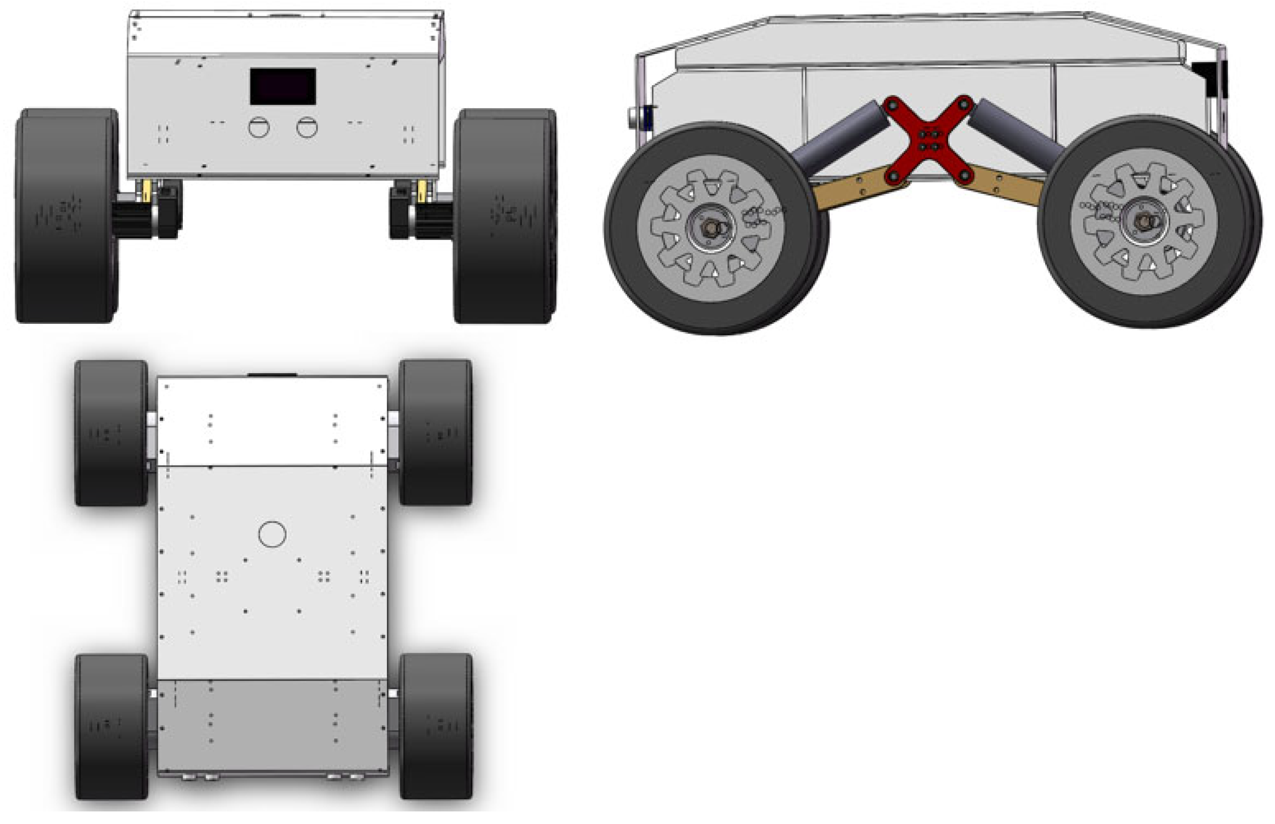
2. Architecture Design of Four-Wheel Adaptive Robot System
2.1. Overall System Design
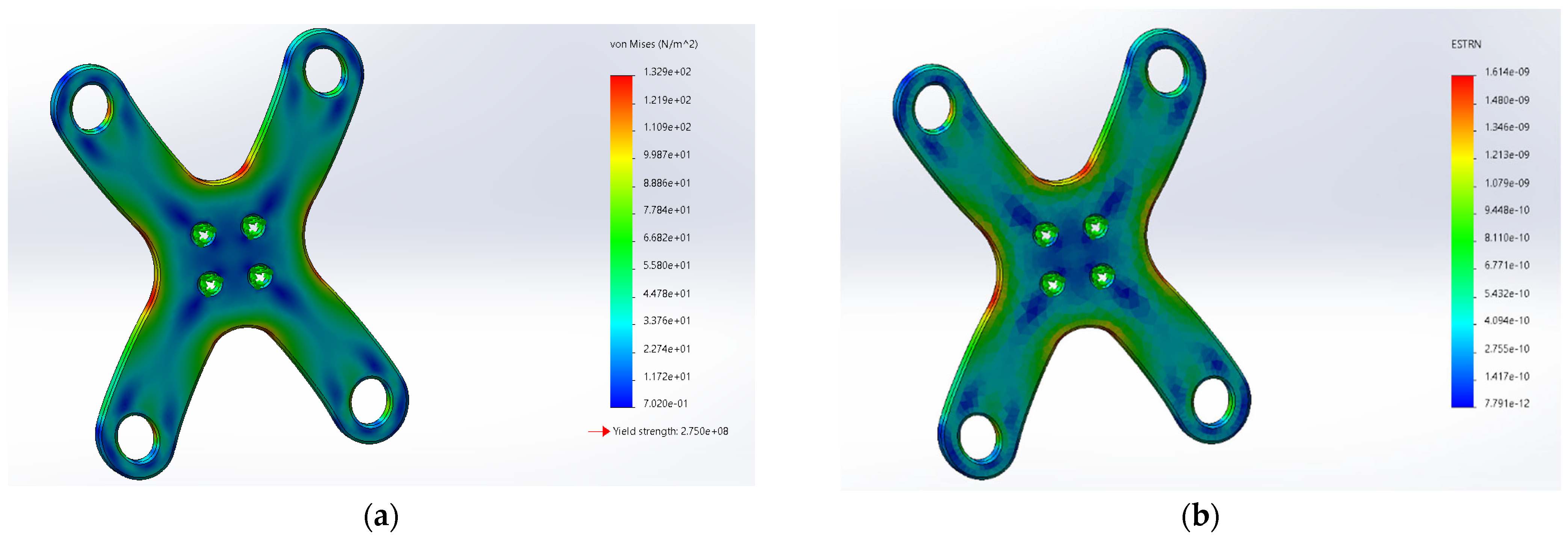
2.2. Analysis of Adaptive Damping Mechanism
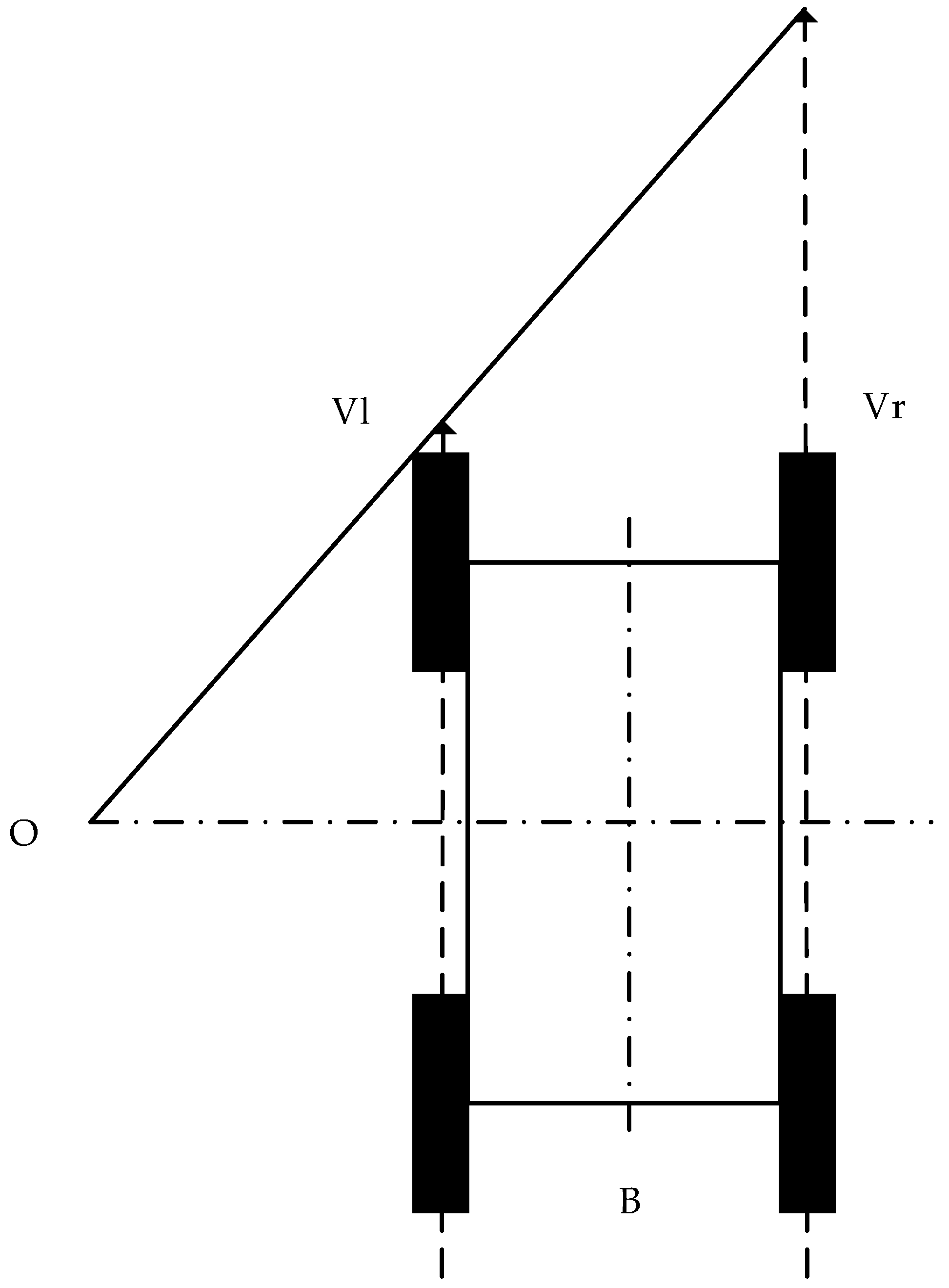
2.3. Adaptive Chassis Steering Analysis
3. Analysis of Four-Wheel Drive Adaptive Robot Algorithm
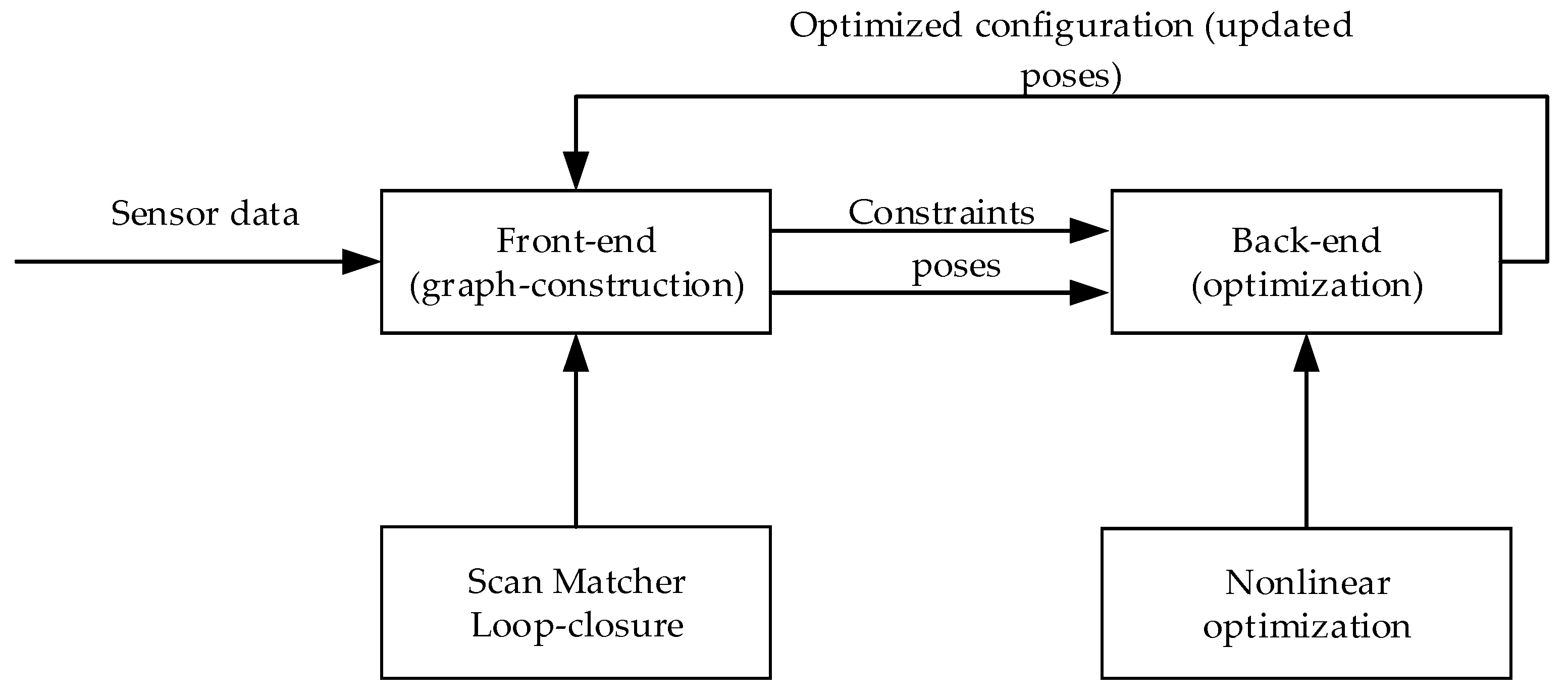
3.1. Introduction to SLAM Algorithms
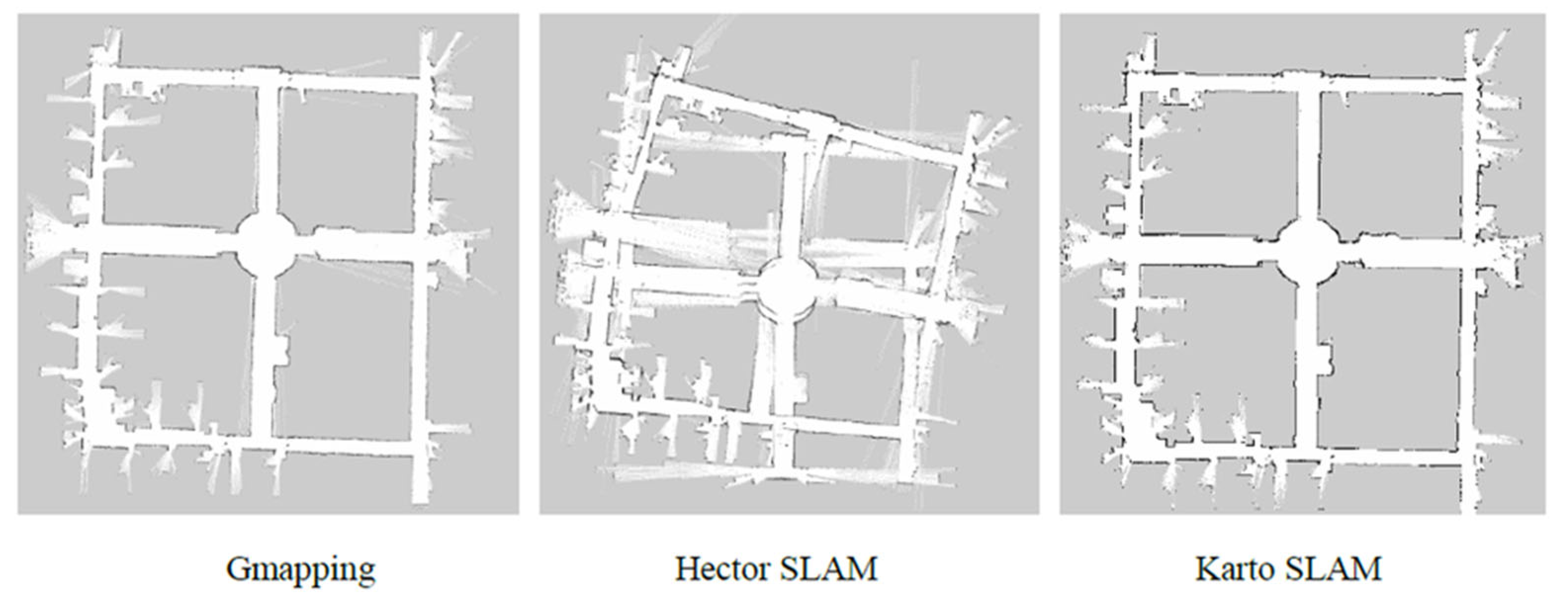
3.1.1. Gmapping Algorithm
3.1.2. Hector SLAM
3.1.3. Karto SLAM
3.2. Introduction to Path Planning Algorithm
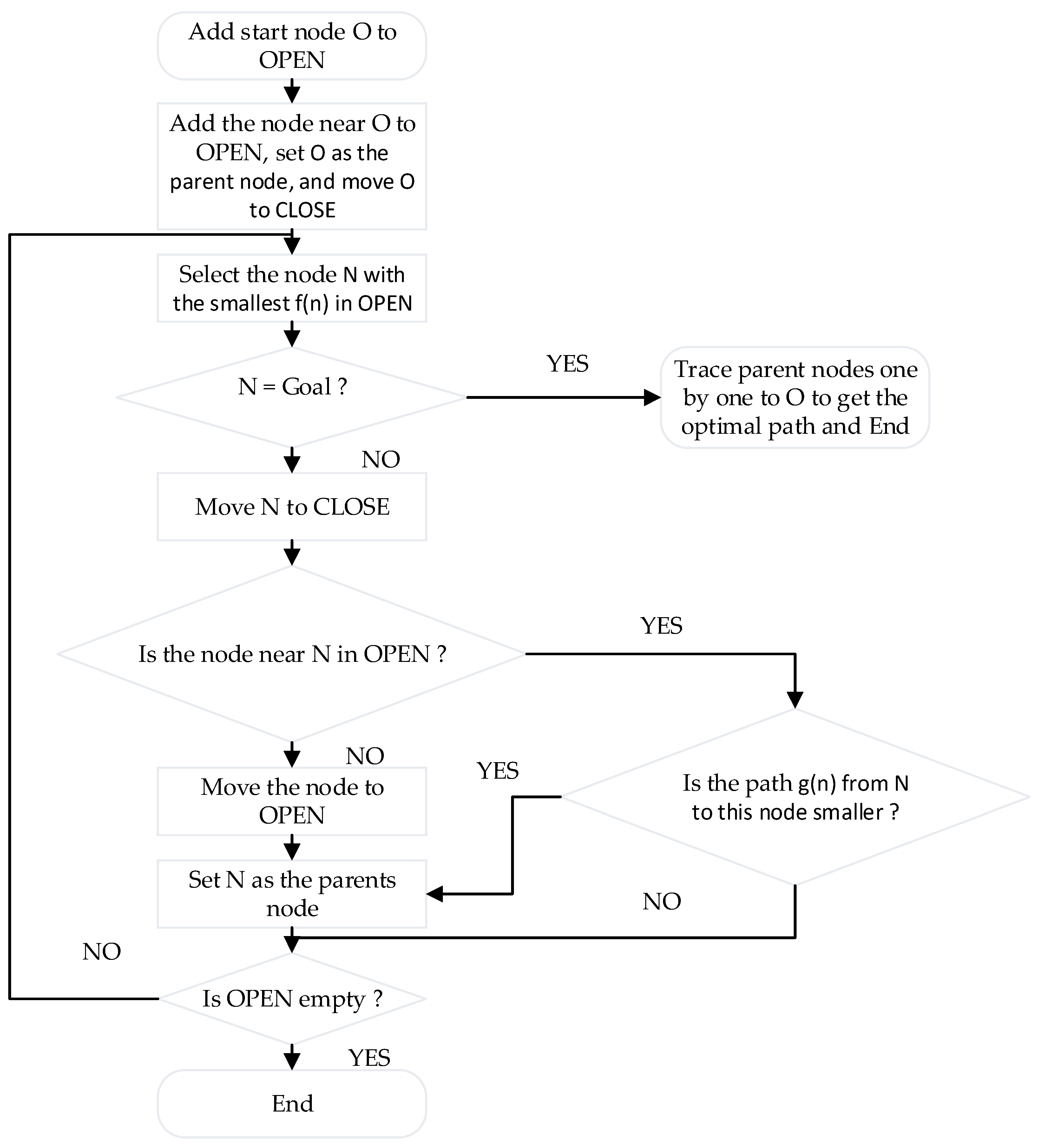
3.2.1. Global Path Planning
3.2.2. Local Path Planning
4. ROS System Simulation of Four-Wheel Drive Adaptive Robot
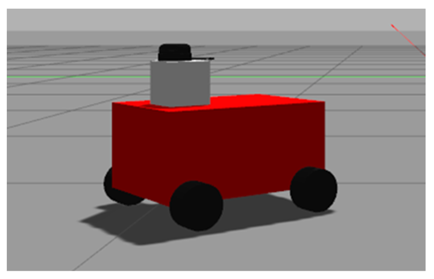
4.1. Establishment of Four-Wheel Drive Adaptive Robot Model
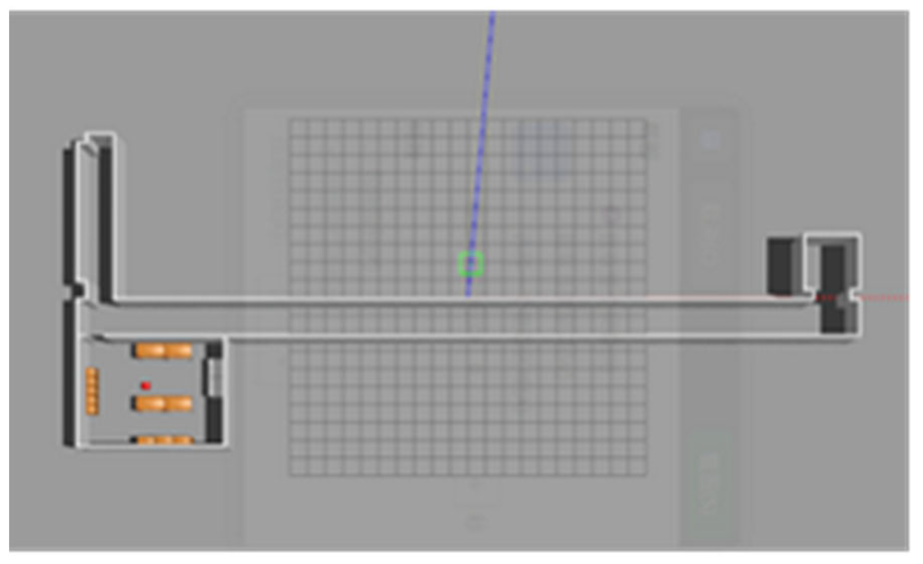
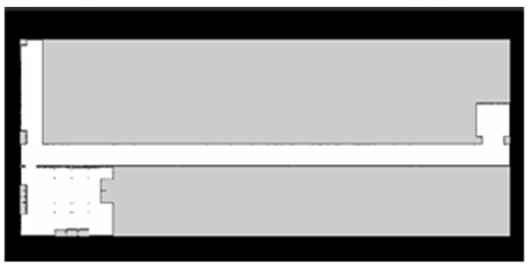
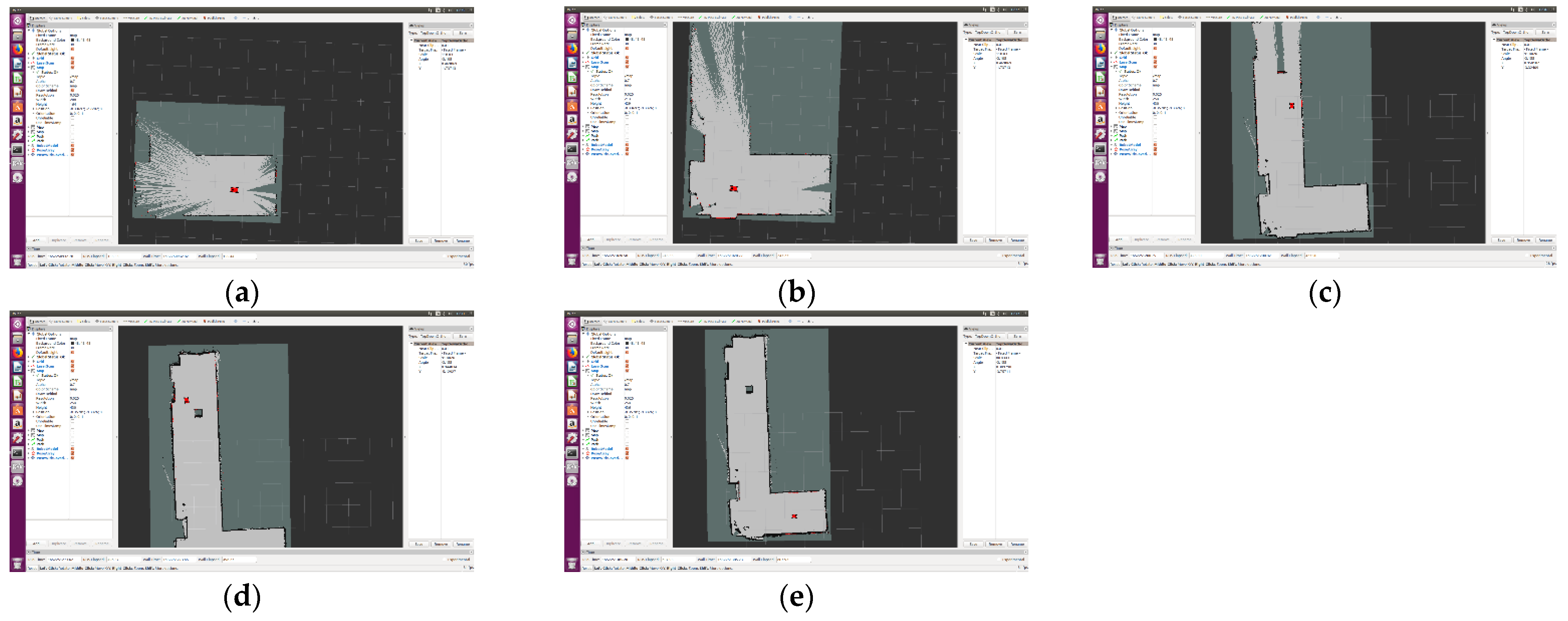
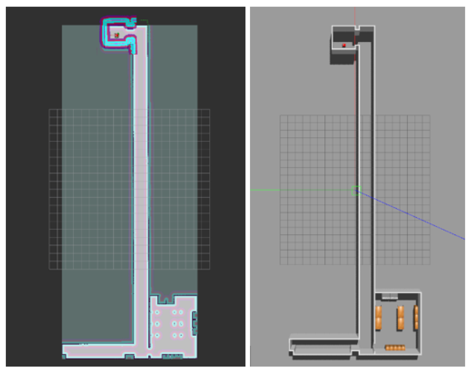
4.2. Mapping Simulation of Four-Wheel Drive Adaptive Robot
4.3. Navigation Simulation of Four-Wheel Drive Adaptive Robot
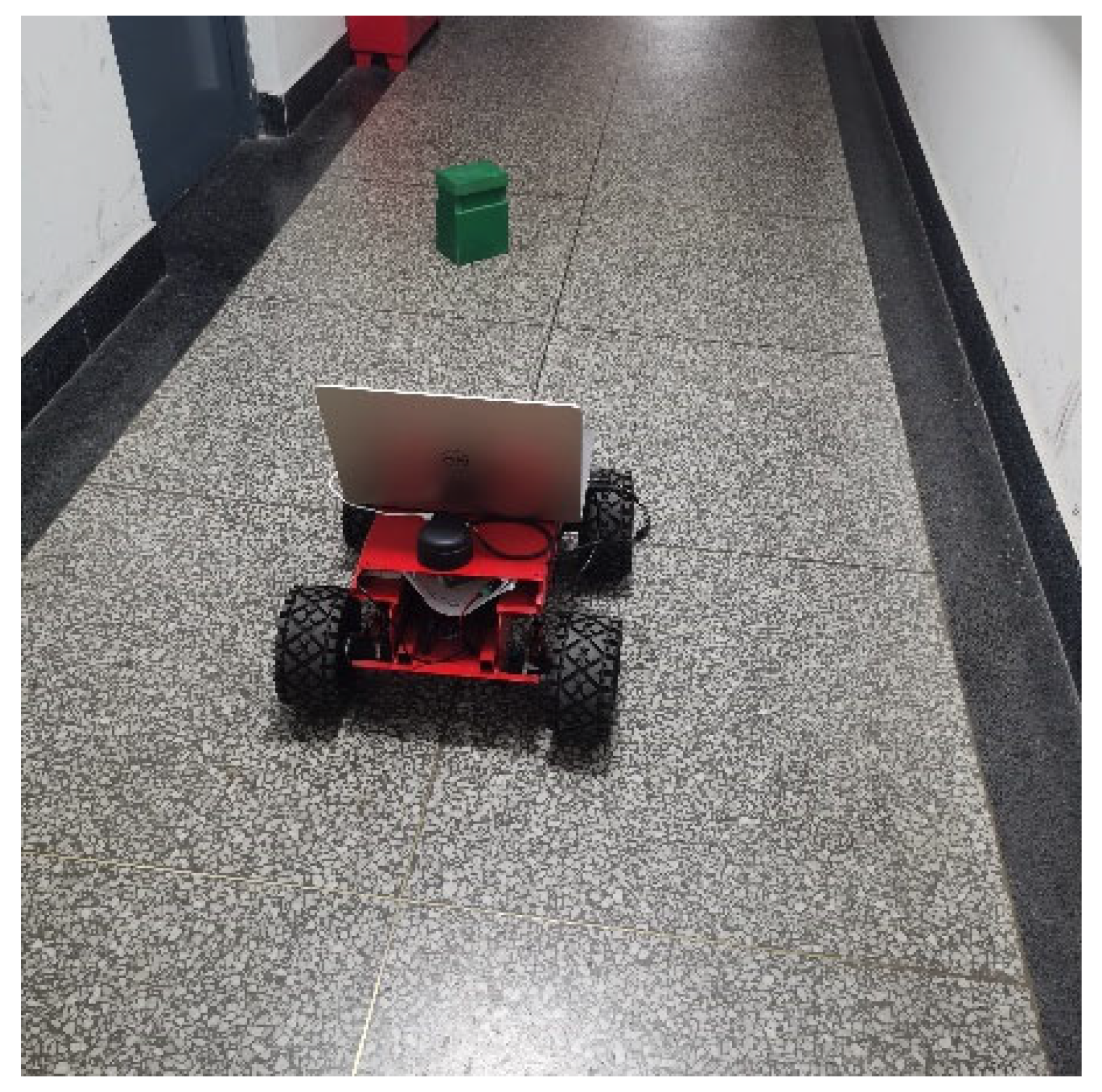
5. Experimental Verification of Four-Wheel Drive Adaptive Robot
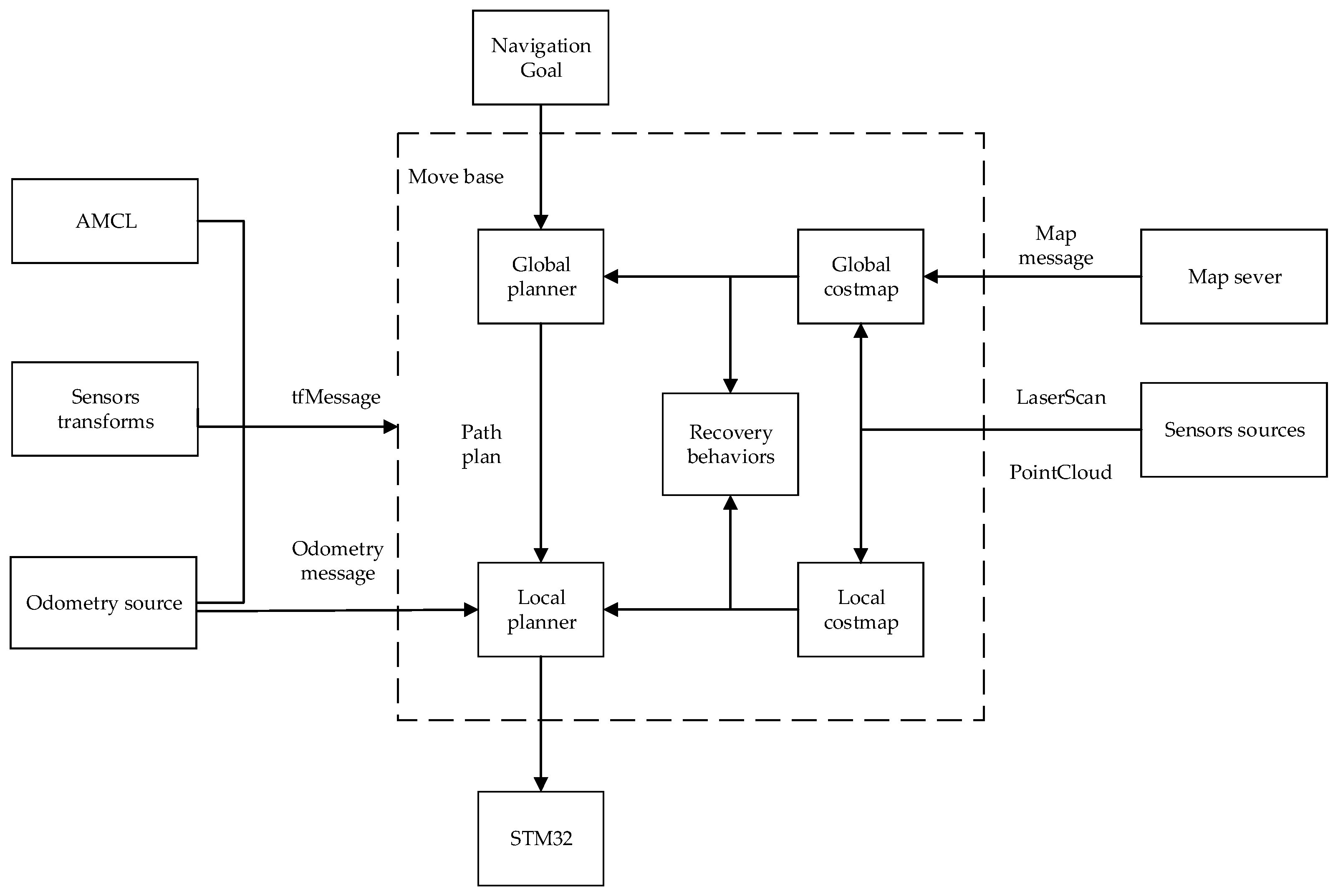
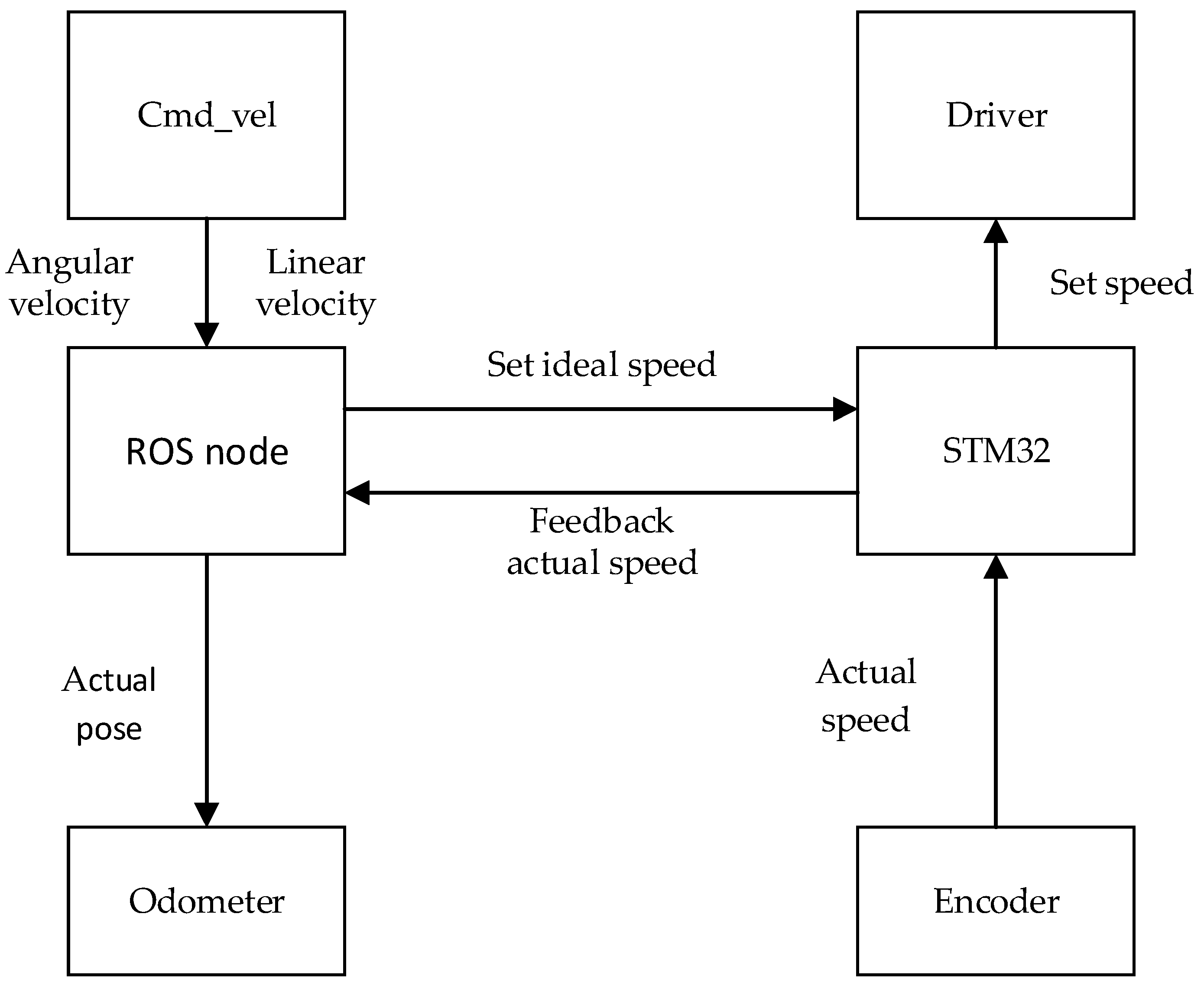
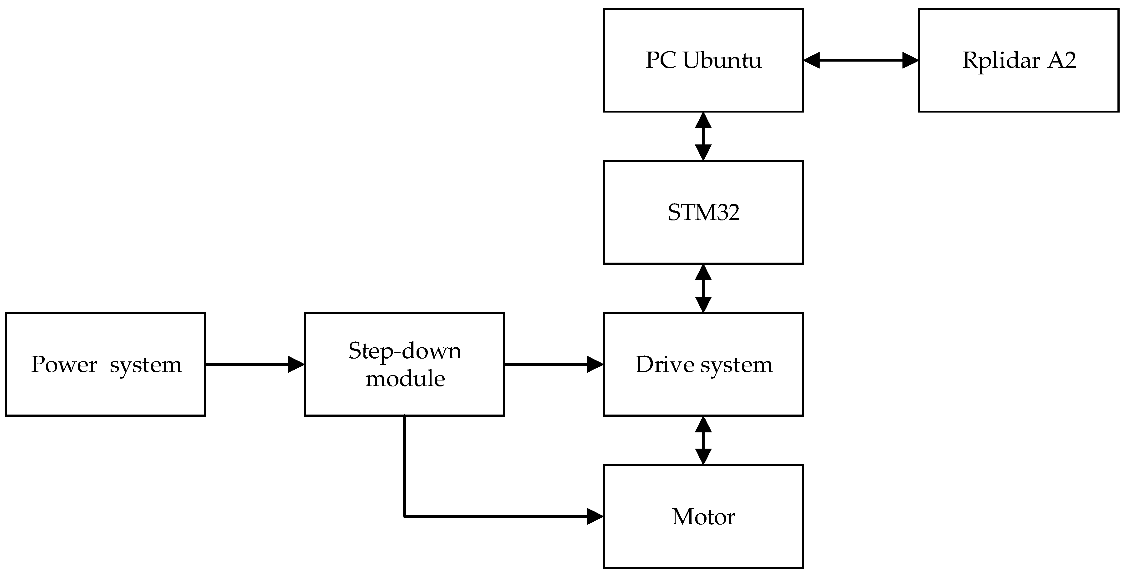
5.1. Chassis Communication and Function Encapsulation
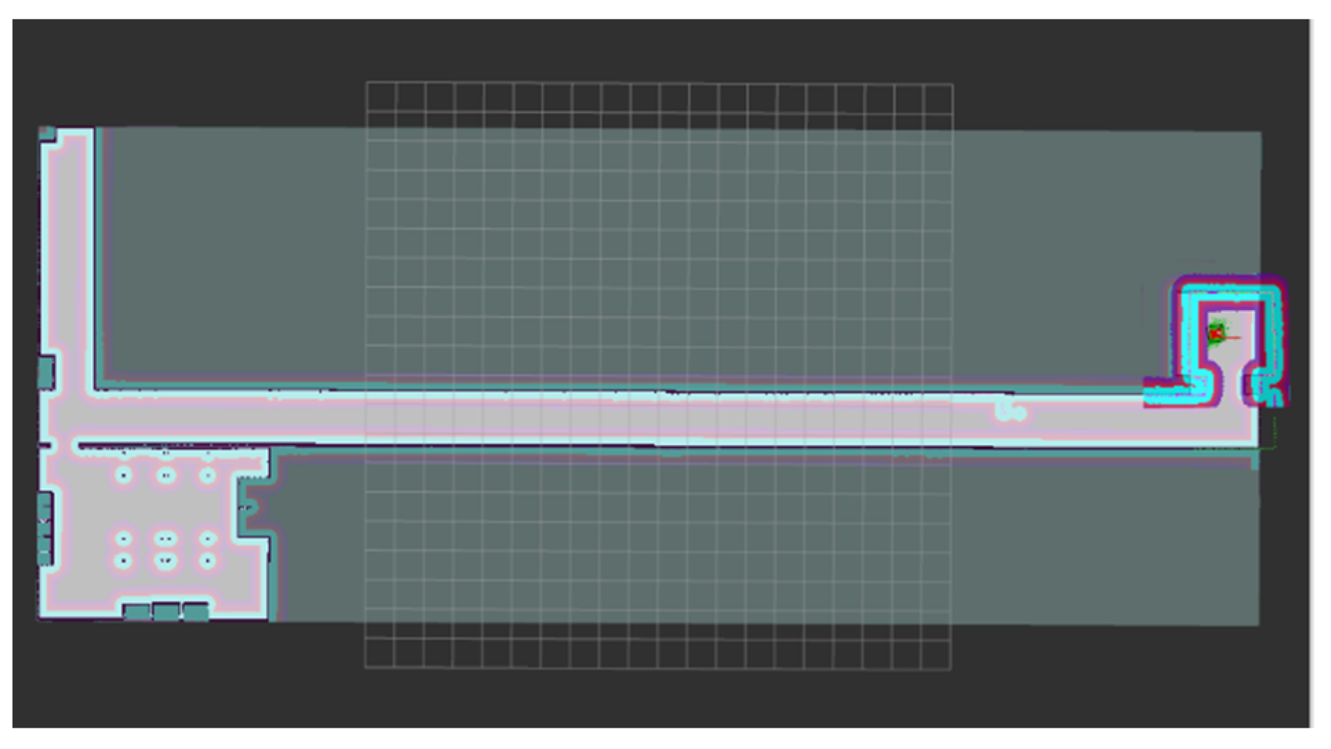
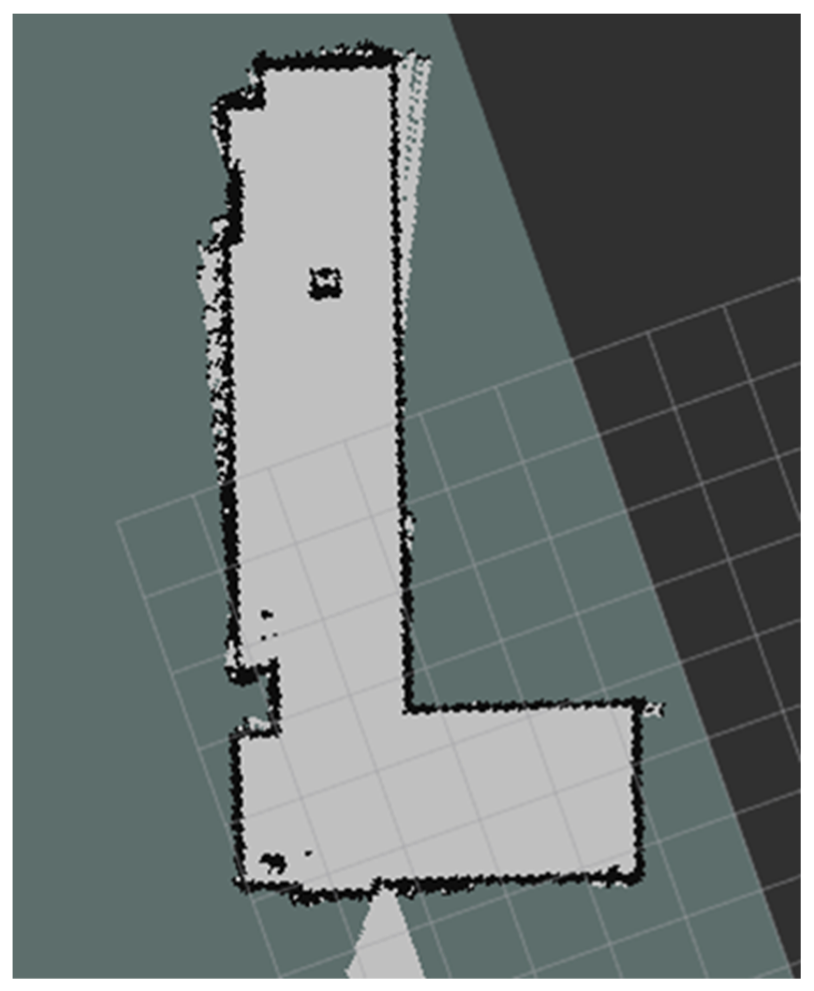
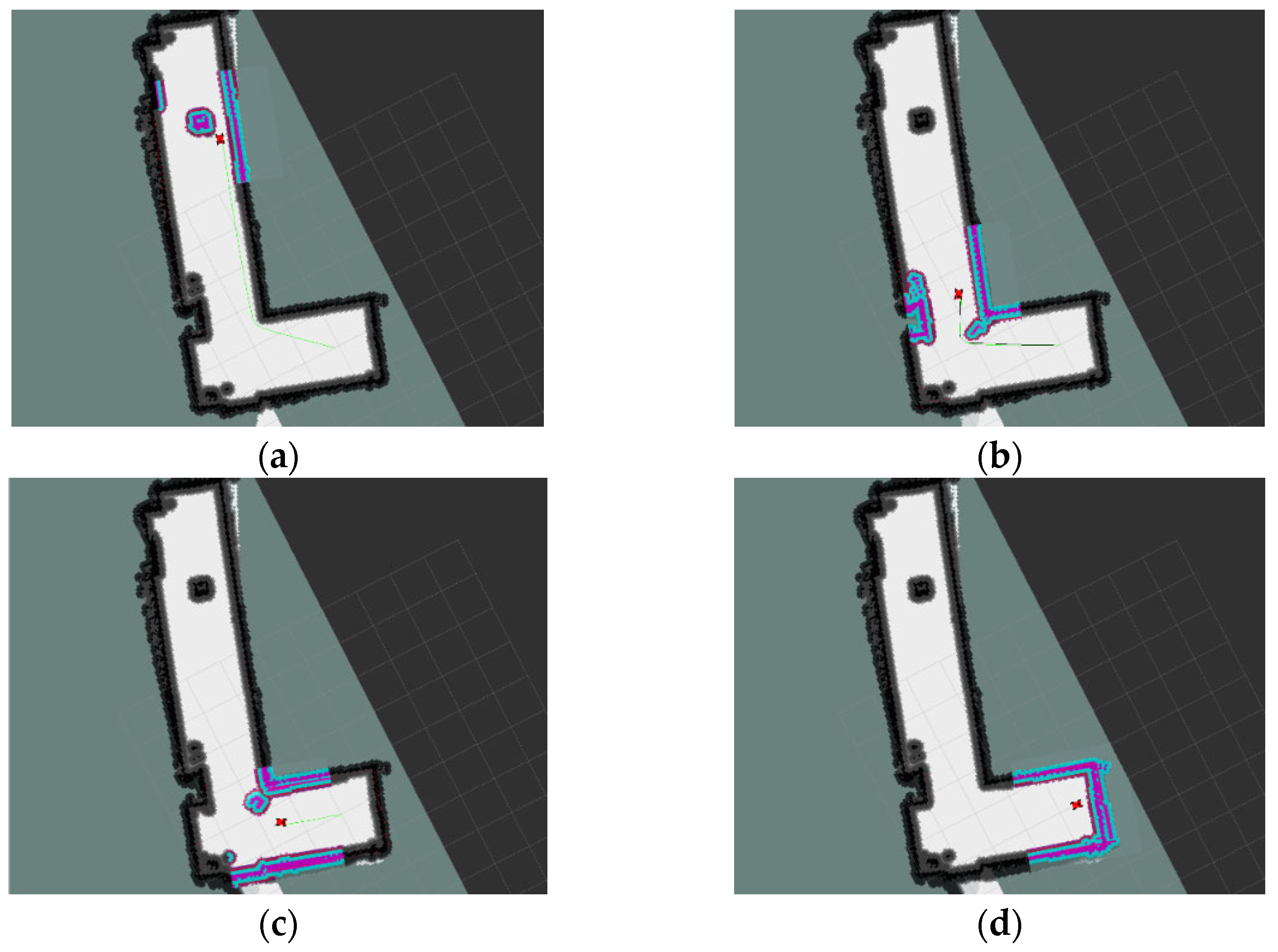
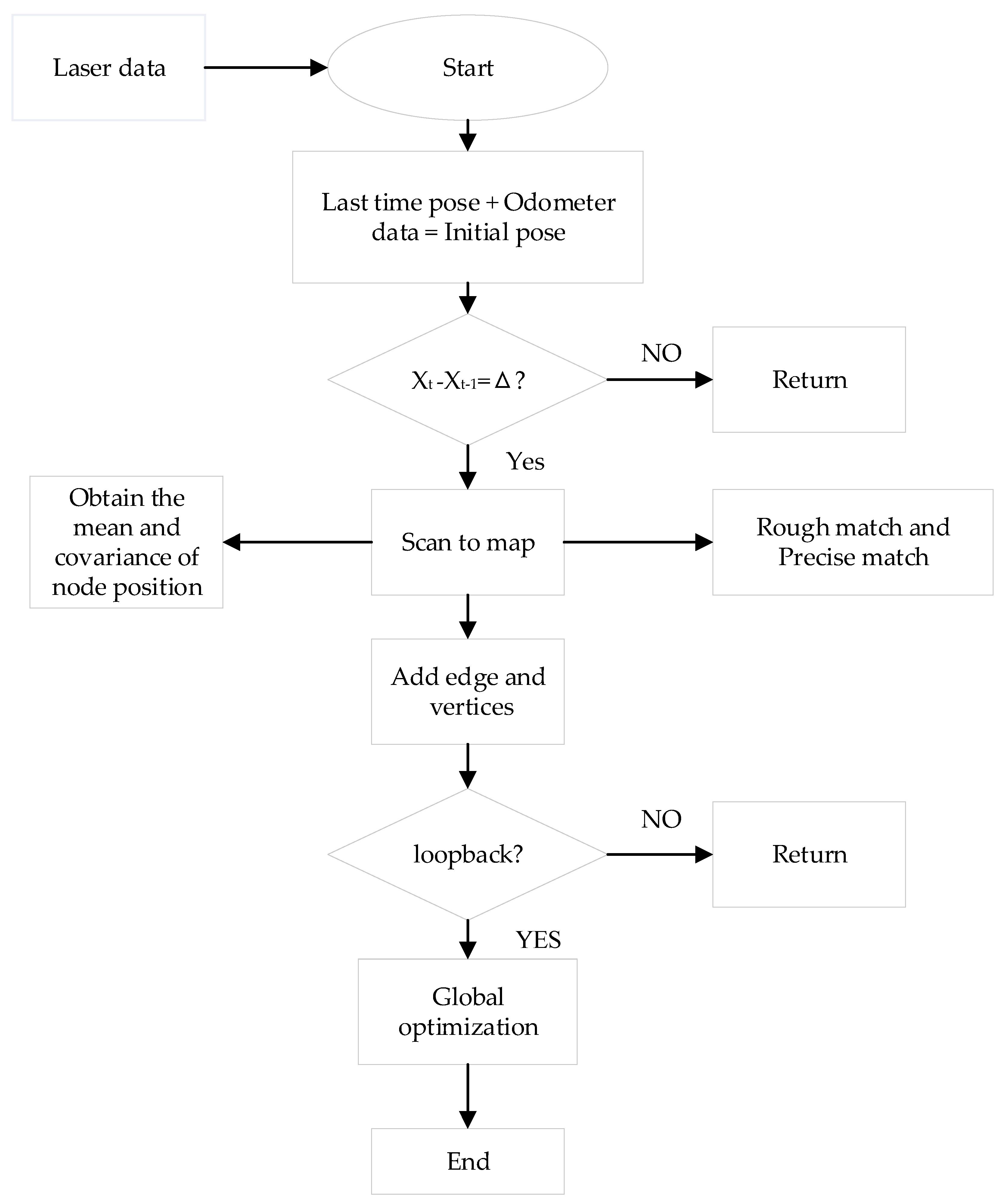
5.2. Mapping and Navigation Experiments
6. System Performance Analysis
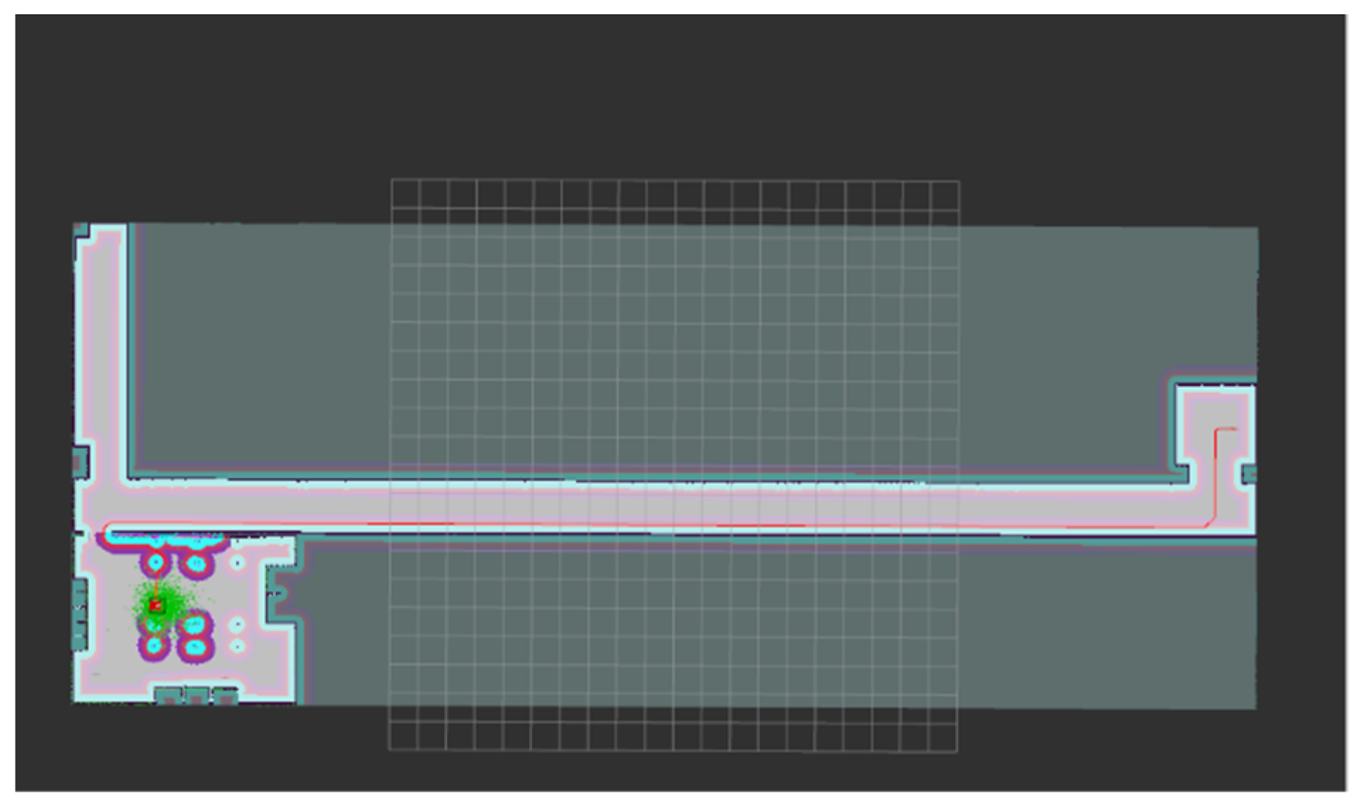
6.1. Simulation Scene Test
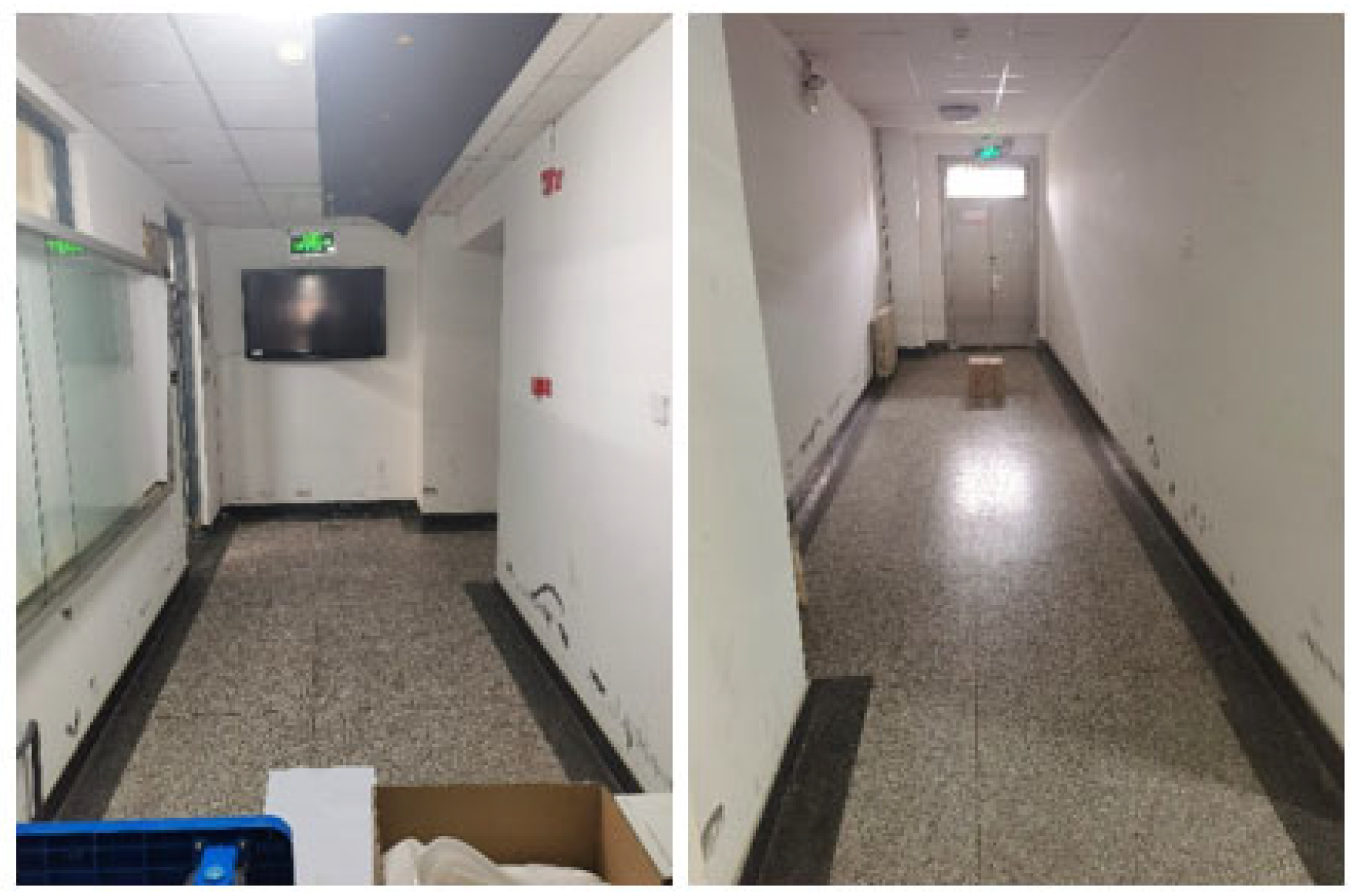
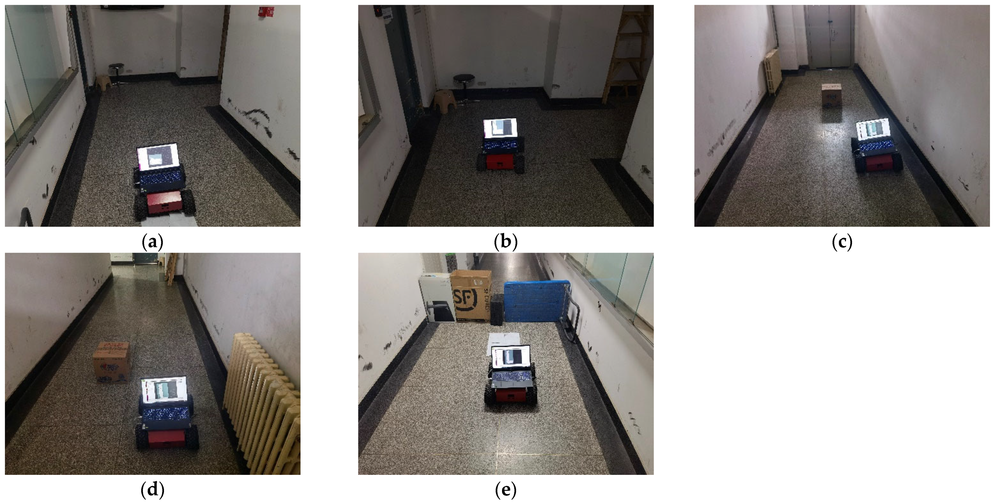
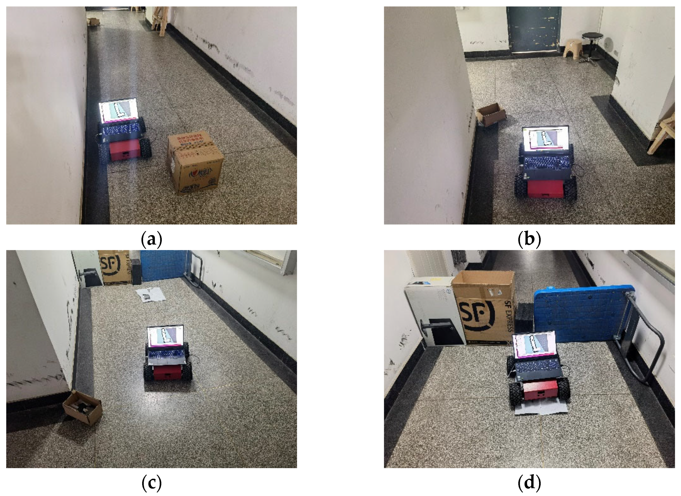
6.2. Actual Scene Test
6.3. Analysis and Discussion
7. Conclusions
Author Contributions
Funding
Institutional Review Board Statement
Informed Consent Statement
Data Availability Statement
Acknowledgments
Conflicts of Interest
References
- Lining, S.; Hui, X.; Zhenhua, W.; Guodong, C. Review on Key Common Technologies for Intelligent Applications of Industrial Robots. J. Vib. Meas. Diagn. 2021, 41, 211–219. [Google Scholar]
- Hongwei, M.; Yan, W.; Lin, Y. Research on Depth Vision Based Mobile Robot Autonomous Navigation in Underground Coal Mine. J. China Coal Soc. 2020, 45, 2193–2206. [Google Scholar]
- Dong, J. Research on SLAM and Navigation for Laser Vision Fusion of Mobile Robot in Indoor Complex Environment. Master’s Thesis, Harbin Institute of Technology, Harbin, China, 2020. [Google Scholar]
- Maosheng, L.; Di, W.; Hao, Y. Deploy Indoor 2D Laser SLAM on a Raspberry Pi-Based Mobile Robot. In Proceedings of the 2019 11th International Conference on Intelligent Human-Machine Systems and Cybernetics (IHMSC), Hangzhou, China, 24–25 August 2019; pp. 7–10. [Google Scholar]
- Peng, W. Research on SLAM Technology and Path Planning Algorithms for Unmanned Vehicle. Master’s Thesis, Harbin Institute of Technology, Harbin, China, 2021. [Google Scholar]
- Jiaxin, S.; Zhiming, Z.; Yongqing, S.; Zheng, Z. Design and Implementation of Indoor Positioning and Navigation System of Mobile Robot Based on ROS and Lidar. Mach. Electron. 2018, 36, 76–80. [Google Scholar]
- Tian, T. Design and Experiment Research of Four Wheel Independent Drive Chassis. Master’s Thesis, Chinese Academy of Agricultural Mechanization Sciences, Beijing, China, 2012. [Google Scholar]
- Yunze, L. Research on SLAM of Indoor Robot Based on Lidar. Master’s Thesis, South China University of Technology, Guangzhou, China, 2016. [Google Scholar]
- Wenzhi, L. Research and Implementation of SLAM and Path Planning Algorithm Based on Lidar. Master’s Thesis, Harbin Institute of Technology, Harbin, China, 2018. [Google Scholar]
- Hanagi, R.R.; Gurav, O.S.; Khandekar, S.A. SLAM using AD* Algorithm with Absolute Odometry. In Proceedings of the 2021 6th International Conference for Convergence in Technology (I2CT), Maharashtra, India, 2–4 April 2021; pp. 1–4. [Google Scholar]
- Zhongli, W.; Jie, Z.; Hegao, C. A Survey of Front-end Method for Graph-based Slam Under Large-scale Environment. J. Harbin Inst. Technol. 2015, 47, 75–85. [Google Scholar]
- Zhang, W.; Zhai, G.; Yue, Z.; Pan, T.; Cheng, R. Research on Visual Positioning of a Roadheader and Construction of an Environment Map. Appl. Sci. 2021, 11, 4968. [Google Scholar] [CrossRef]
- Johannsson, H.; Kaess, M.; Fallon, M.; Leonard, J.J. Temporally Scalable Visual SLAM Using a Reduced Pose Graph. In Proceedings of the 2013 IEEE International Conference on Robotics and Automation, Karlsruhe, Germany, 6–10 May 2013. [Google Scholar]
- Zhiguo, Z.; Jiangwei, C.; Shunfan, D. Overview of 3D Lidar SLAM algorithms. Chin. J. Sci. Instrum. 2021, 42, 13–27. [Google Scholar]
- Han, D.; Li, Y.; Song, T.; Liu, Z. Multi-Objective Optimization of Loop Closure Detection Parameters for Indoor 2D Simultaneous Localization and Mapping. Sensors 2020, 20, 1906. [Google Scholar] [CrossRef] [PubMed] [Green Version]
- SLAM Benchmarking. Available online: http://ais.informatik.uni-freiburg.de/slamevaluation/datasets.php (accessed on 27 November 2020).
- Verma, D.; Messon, D.; Rastogi, M.; Singh, A. Comparative Study of Various Approaches Of Dijkstra Algorithm. In Proceedings of the 2021 International Conference on Computing, Communication, and Intelligent Systems (ICCCIS), Greater Noida, India, 19–20 February 2021. [Google Scholar]
- Foead, D.; Ghifari, A.; Kusuma, M.B.; Hanafiah, N.; Gunawan, E. A Systematic Literature Review of A* Pathfinding. Procedia Comput. Sci. 2021, 179, 507–514. [Google Scholar] [CrossRef]
- Zhao, X.; Wang, Z.; Huang, C.K.; Zhao, Y.W. Mobile Robot Path Planning Based on an Improved A* Algorithm. Robot 2018, 40, 903–910. [Google Scholar]
- Wang, H.; Yin, P.; Zheng, W.; Wang, H.; Zuo, J. Mobile Robot Path Planning Based on Improved A* Algorithm and Dynamic Window Method. Robot 2020, 42, 346–353. [Google Scholar]
- Cailian, L.; Peng, L.; Yu, F. Path Planning of Greenhouse Robot Based on Fusion of Improved A* Algorithm and Dynamic Window Approach. Trans. Chin. Soc. Agric. Mach. 2021, 52, 14–22. [Google Scholar]
- Si, L.; Xunhao, Z.; Xinyang, Z.; Chao, T. Kinematics Analysis and Whole Positioning Method of Logistics Robot. J. Hunan Inst. Sci. Technol. (Nat. Sci.) 2020, 33, 32–37. [Google Scholar]
- Chengyu, L. Research on Trajectory Tracking Control of Four-wheel Sliding Steering Robot. Master’s Thesis, Dalian Maritime University, Dalian, China, 2017. [Google Scholar]
- Song, K.; Chiu, Y.; Kang, L. Navigation control design of a mobile robot by integrating obstacle avoidance and LiDAR SLAM. In Proceedings of the 2018 IEEE International Conference on Systems, Man, and Cybernetics (SMC), Miyazaki, Japan, 7–10 October 2018; pp. 1833–1838. [Google Scholar]
- Savkin, A.V.; Hang, L. A safe area search and map building algorithm for a wheeled mobile robot in complex unknown cluttered environments. Robotica 2018, 36, 96–118. [Google Scholar] [CrossRef]
- Yongbo, C.; Shoudong, H.; Fitch, R. Active SLAM for mobile robots with area coverage and obstacle avoidance. IEEE/ASME Trans. Mechatron. 2020, 25, 1182–1192. [Google Scholar]
- Kan, X.; Teng, H.; Karydis, K. Online Exploration and Coverage Planning in Unknown Obstacle-Cluttered Environments. IEEE Robot. Autom. Lett. 2020, 5, 5969–5976. [Google Scholar] [CrossRef]


| Module | Model |
|---|---|
| Chassis | Four-wheel differential chassis |
| Motor | Faulhaber Dc servo motor |
| Motor driver | Rmds-108 DC servo motor driver |
| Controller | STM32F103 |
| Lidar | Rplidar_A2 |
| Algorithm Name | Gmapping | Hector SLAM | Karto SLAM |
|---|---|---|---|
| Principle | Filter | Optimization | Graph optimization |
| Lidar frequency requirement | Low | High | Low |
| Odometer accuracy requirement | High | No | Low |
| Loopback | No | No | Yes |
| Robustness | High | Low | High |
| The Plugin Name | Description |
|---|---|
| libgazebo_ros_skid_steer_drive.so | Sliding steering motion plugin |
| libgazebo_ros_imu.so | IMU sensor plugin |
| libgazebo_ros_laser.so | Lader plugin |
| Libgazebo_ros_skid_steer_drive.so | Sliding steering motion plugin |
| libgazebo_ros_imu.so | IMU sensor plugin |
| libgazebo_ros_laser.so | Lader plugin |
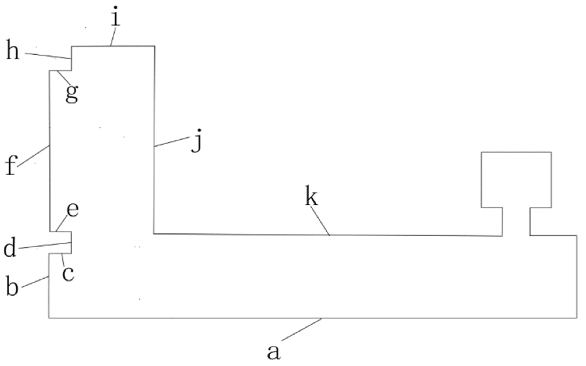
| Number | True Value (m) | Measurement 1 (m) | Measurement 2 (m) | Measurement 3 (m) | Mean of Measurements (m) | Absolute Error (m) | Relative Error (%) |
|---|---|---|---|---|---|---|---|
| a | 41.000 | 40.287 | 40.036 | 40.266 | 40.196 | −0.804 | 2.01 |
| b | 1.850 | 1.796 | 1.840 | 1.842 | 1.826 | −0.024 | 1.30 |
| c | 0.500 | 0.498 | 0.496 | 0.497 | 0.497 | −0.003 | 0.60 |
| d | 1.150 | 1.167 | 1.157 | 1.156 | 1.160 | 0.010 | 0.87 |
| e | 0.500 | 0.497 | 0.496 | 0.498 | 0.497 | −0.003 | 0.60 |
| f | 7.350 | 7.279 | 7.334 | 7.332 | 7.315 | −0.035 | 0.48 |
| g | 0.500 | 0.498 | 0.495 | 0.496 | 0.496 | −0.004 | 0.80 |
| h | 0.500 | 0.502 | 0.494 | 0.498 | 0.498 | −0.002 | 0.40 |
| i | 1.350 | 1.293 | 1.295 | 1.297 | 1.295 | −0.055 | 4.07 |
| j | 9.000 | 8.996 | 8.946 | 8.998 | 8.980 | −0.020 | 0.22 |
| k | 38.150 | 37.500 | 37.277 | 37.335 | 37.371 | −0.779 | 2.04 |
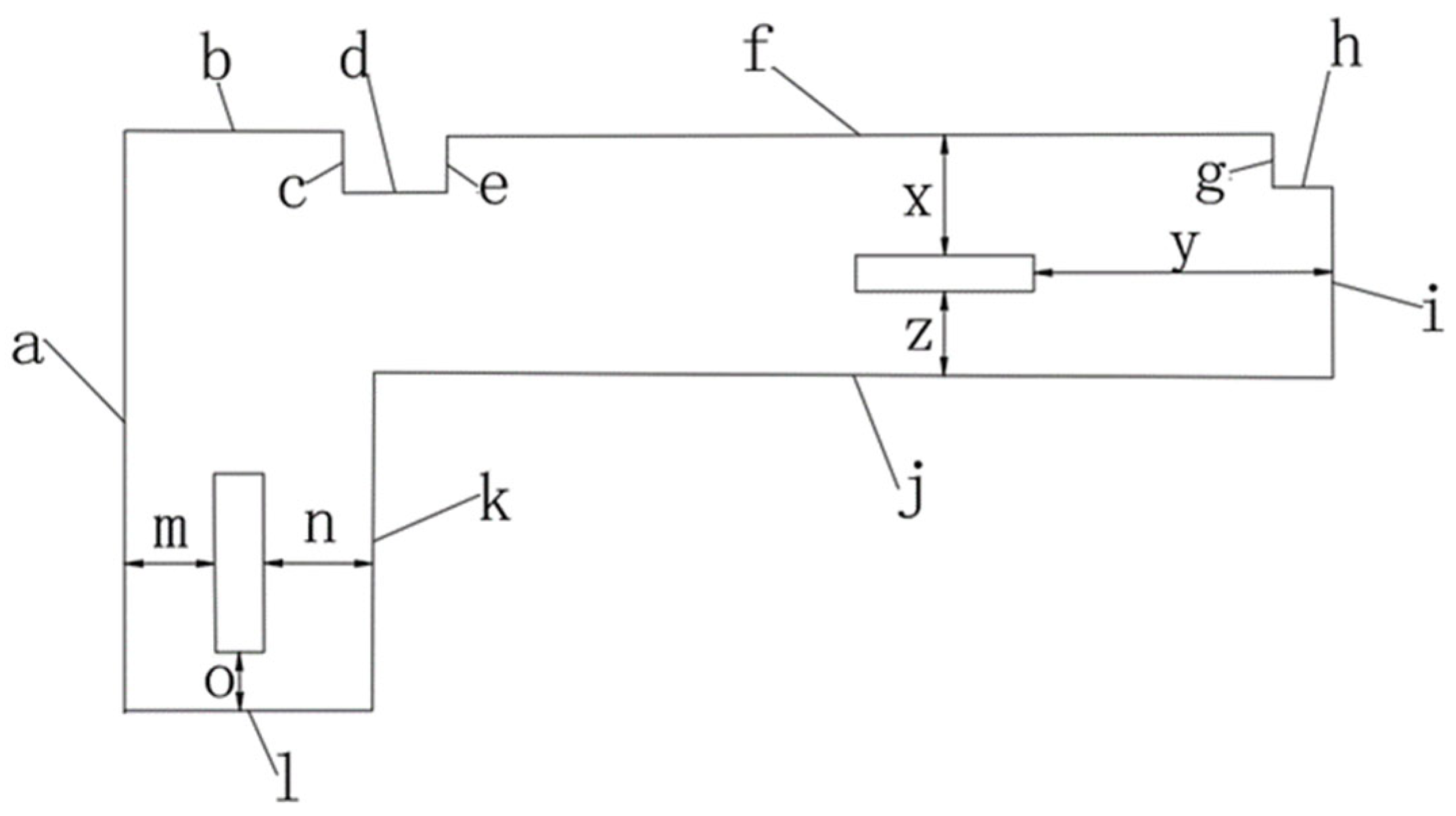
| Number | True Value (m) | Measurement 1 (m) | Measurement 2 (m) | Measurement 3 (m) | Mean of Measurements (m) | Absolute Error (m) | Relative Error (%) |
|---|---|---|---|---|---|---|---|
| a | 4.900 | 4.877 | 4.882 | 4.886 | 4.882 | −0.018 | 0.37 |
| b | 1.830 | 1.902 | 1.780 | 1.840 | 1.841 | 0.011 | 0.60 |
| c | 0.515 | 0.546 | 0.502 | 0.508 | 0.519 | 0.004 | 0.78 |
| d | 0.870 | 0.885 | 0.890 | 0.876 | 0.884 | 0.014 | 1.61 |
| e | 0.470 | 0.510 | 0.478 | 0.476 | 0.488 | 0.018 | 3.83 |
| f | 6.930 | 6.898 | 6.895 | 6.902 | 6.898 | −0.032 | 0.46 |
| g | 0.445 | 0.510 | 0.452 | 0.456 | 0.473 | 0.018 | 4.04 |
| h | 0.500 | 0.428 | 0.484 | 0.495 | 0.469 | −0.031 | 6.20 |
| i | 1.600 | 1.582 | 1.586 | 1.591 | 1.586 | −0.014 | 0.88 |
| j | 8.050 | 7.982 | 8.020 | 8.032 | 8.011 | −0.039 | 0.48 |
| k | 2.840 | 2.795 | 2.828 | 2.832 | 2.818 | −0.022 | 0.77 |
| l | 2.080 | 2.020 | 2.090 | 2.092 | 2.067 | −0.013 | 0.63 |
| x | 1.015 | 1.004 | 1.005 | 1.007 | 1.005 | −0.010 | 0.99 |
| y | 2.500 | 2.478 | 2.486 | 2.488 | 2.484 | −0.016 | 0.64 |
| z | 0.700 | 0.674 | 0.829 | 0.683 | 0.732 | 0.032 | 4.57 |
| m | 0.750 | 0.735 | 0.738 | 0.736 | 0.736 | −0.014 | 1.87 |
| n | 0.910 | 0.922 | 0.934 | 0.937 | 0.931 | 0.021 | 2.31 |
| o | 0.490 | 0.470 | 0.476 | 0.468 | 0.471 | −0.019 | 3.88 |
| θ | 0° | 15.0° | 6.0° | −8.0° | 4.3° | 4.3° |
Publisher’s Note: MDPI stays neutral with regard to jurisdictional claims in published maps and institutional affiliations. |
© 2022 by the authors. Licensee MDPI, Basel, Switzerland. This article is an open access article distributed under the terms and conditions of the Creative Commons Attribution (CC BY) license (https://creativecommons.org/licenses/by/4.0/).
Share and Cite
Zhao, J.; Liu, S.; Li, J. Research and Implementation of Autonomous Navigation for Mobile Robots Based on SLAM Algorithm under ROS. Sensors 2022, 22, 4172. https://doi.org/10.3390/s22114172
Zhao J, Liu S, Li J. Research and Implementation of Autonomous Navigation for Mobile Robots Based on SLAM Algorithm under ROS. Sensors. 2022; 22(11):4172. https://doi.org/10.3390/s22114172
Chicago/Turabian StyleZhao, Jianwei, Shengyi Liu, and Jinyu Li. 2022. "Research and Implementation of Autonomous Navigation for Mobile Robots Based on SLAM Algorithm under ROS" Sensors 22, no. 11: 4172. https://doi.org/10.3390/s22114172
APA StyleZhao, J., Liu, S., & Li, J. (2022). Research and Implementation of Autonomous Navigation for Mobile Robots Based on SLAM Algorithm under ROS. Sensors, 22(11), 4172. https://doi.org/10.3390/s22114172