
Wearable Sensor Based on Flexible Sinusoidal Antenna for Strain Sensing Applications


Abstract
:1. Introduction
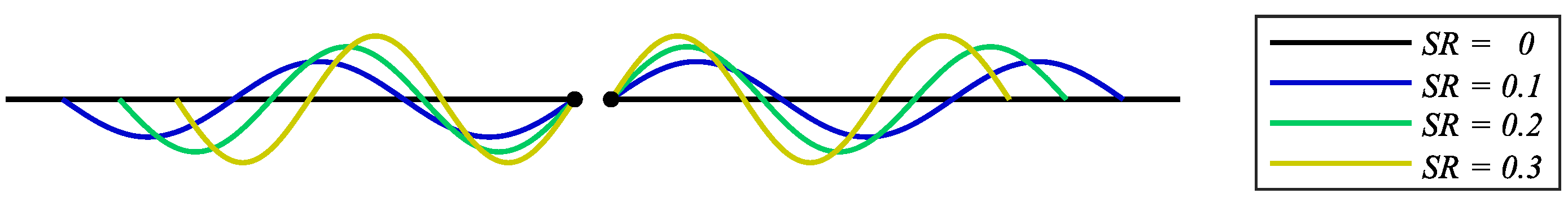
2. Antenna Geometry
3. Specifications and Intrinsic Parameters
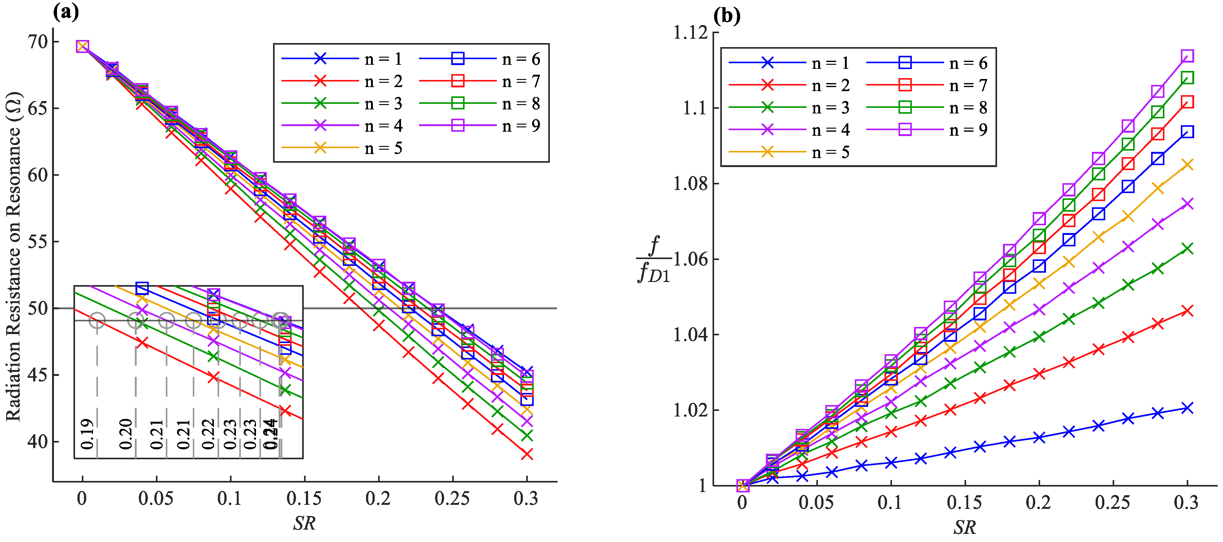
3.1. Radiation Resistance
3.2. Resonance Frequency
3.3. Effects of the Factor
3.4. Radiation Pattern and Maximum Gain
4. Design Methods
4.1. Method 1: Designing Based on for a Known
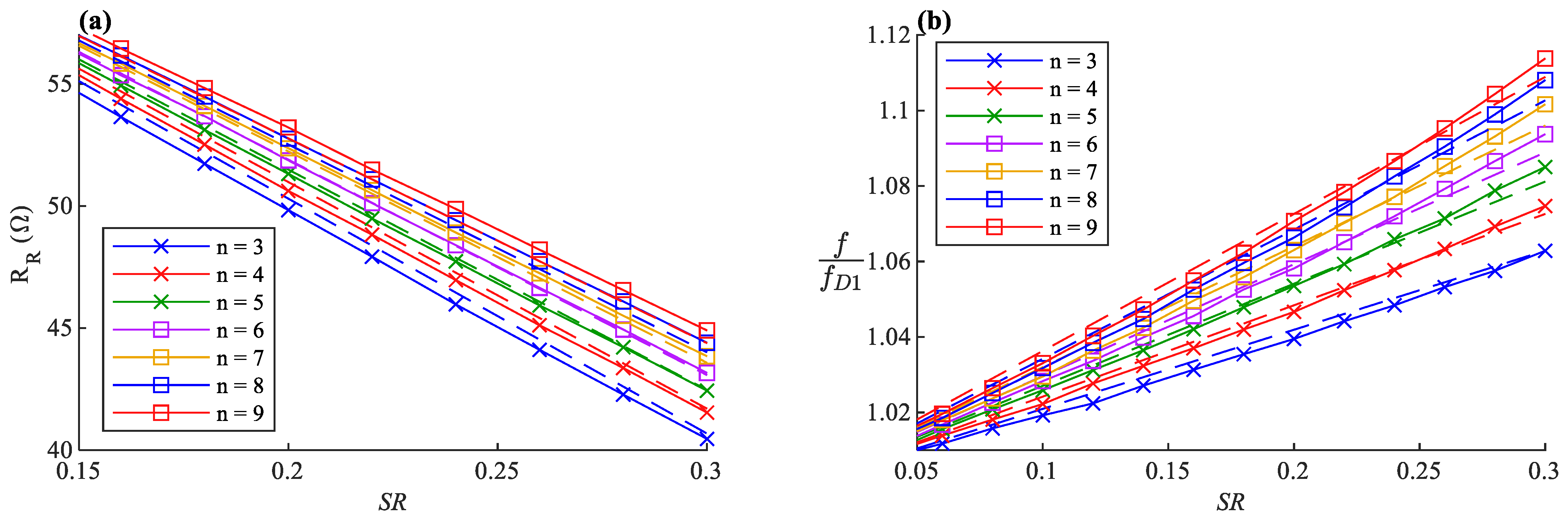
4.1.1. Curve Fittings Based on
4.1.2. The Design Steps Using Method 1
- Choosing a wire length and
- Calculating for different values, or calculate for a given
- Calculating for the chosen in step 2
- Readjusting (and subsequently updating ) while keeping fixed to reach the desired resonance frequency
- Calculating based on the finalized and using the integral Equation introduced in the following.
- Verify the design by simulating the antenna model based on Equation (1)
- Finish if the desired frequency is acquired; otherwise, repeat from Step 4.
4.1.3. Calculating Antenna width
4.1.4. Disadvantages of Method 1 Based on
4.2. Method 2: Designing Based on for a Known
4.2.1. Widening Ratio
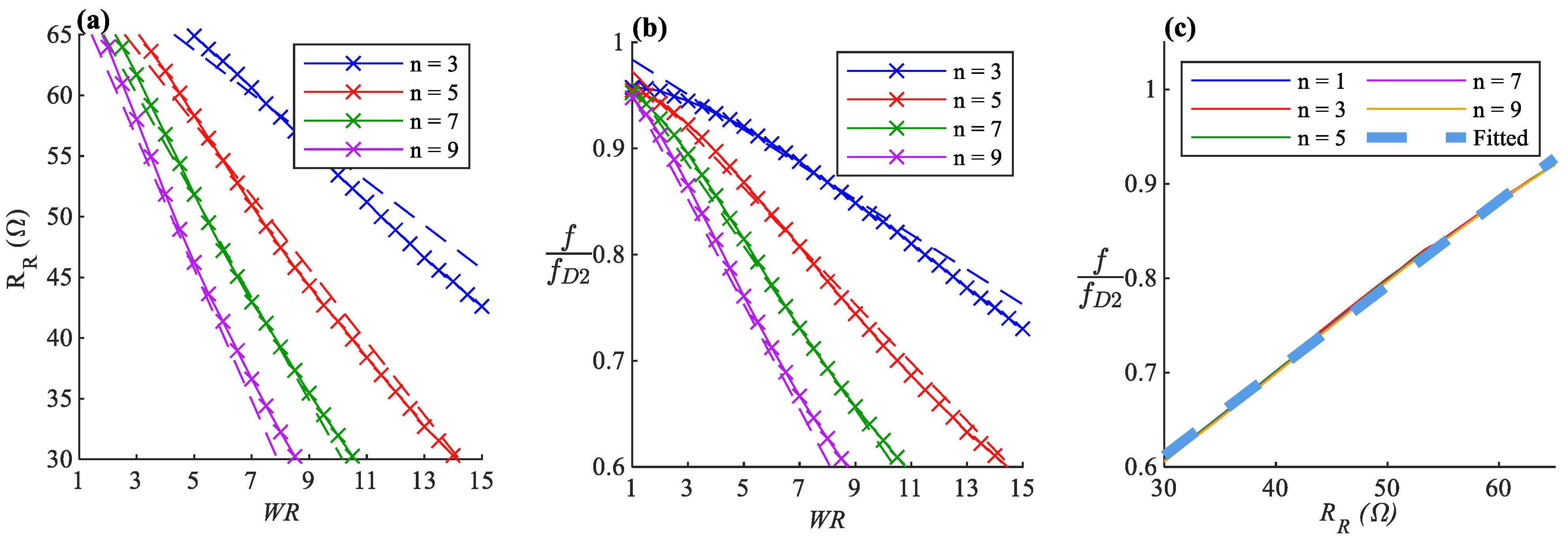
4.2.2. Curve Fittings Based on
4.2.3. The Design Steps Using Method 2
- Choosing a wire length and
- Calculating for different values, or calculate for a given
- Calculating for the chosen in step 2
- Readjusting (and subsequently updating ) while keeping fixed to reach the desired resonance frequency
- Verify the design by simulating the antenna model based on Equation (1)
- Finish if the desired frequency is acquired; otherwise, repeat from Step 4.
4.2.4. Advantages of Method 2 Based on
4.3. Tuning Considerations
5. Fabrication and Measurement
5.1. Fabrication Process
5.2. Measurements
5.3. The Durability of the Antenna Sensor
6. Discussion
6.1. Strain Sensitivity
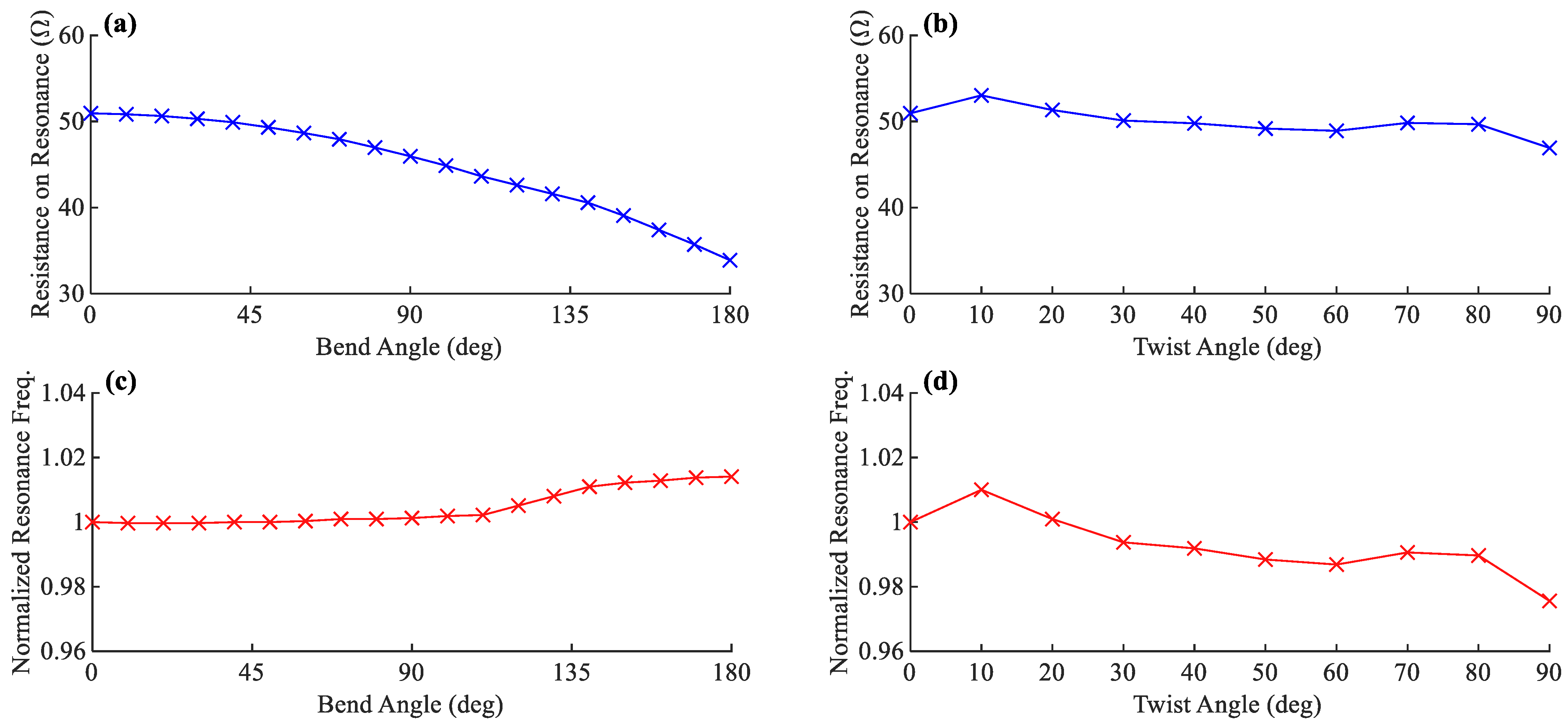
6.2. Effects of Bending and Twisting
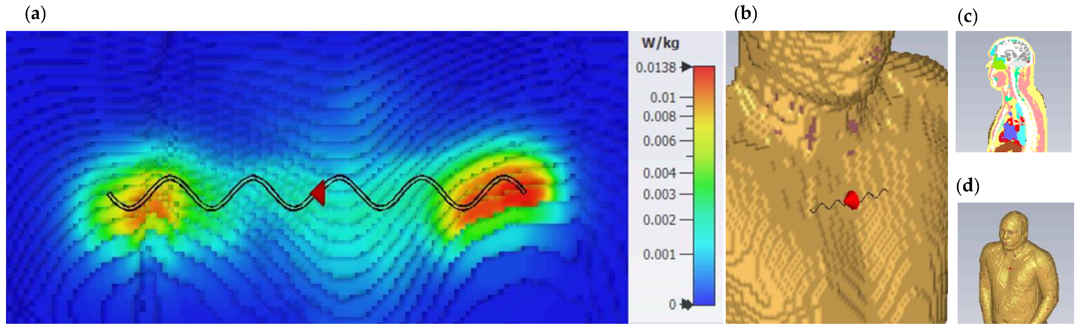
6.3. Specific Absorption Rate (SAR) Analysis
7. Conclusions
Author Contributions
Funding
Institutional Review Board Statement
Informed Consent Statement
Conflicts of Interest
Appendix A
References
- Kraus, J.D. Antennas, 2nd ed.; McGraw-Hill Series in Electrical Engineering; McGraw-Hill: New York, NY, USA, 1988; ISBN 978-0-07-035422-7. [Google Scholar]
- Roudjane, M.; Bellemare-Rousseau, S.; Khalil, M.; Gorgutsa, S.; Miled, A.; Messaddeq, Y. A Portable Wireless Communication Platform Based on a Multi-Material Fiber Sensor for Real-Time Breath Detection. Sensors 2018, 18, 973. [Google Scholar] [CrossRef] [PubMed] [Green Version]
- Roudjane, M.; Bellemare-Rousseau, S.; Drouin, E.; Belanger-Huot, B.; Dugas, M.-A.; Miled, A.; Messaddeq, Y. Smart T-Shirt Based on Wireless Communication Spiral Fiber Sensor Array for Real-Time Breath Monitoring: Validation of the Technology. IEEE Sens. J. 2020, 20, 10841–10850. [Google Scholar] [CrossRef]
- Guay, P.; Gorgutsa, S.; LaRochelle, S.; Messaddeq, Y. Wearable Contactless Respiration Sensor Based on Multi-Material Fibers Integrated into Textile. Sensors 2017, 17, 1050. [Google Scholar] [CrossRef] [PubMed]
- Mulholland, K.; Virkki, J.; Raumonen, P.; Merilampi, S. Wearable RFID Perspiration Sensor Tags for Well-Being Applications—From Laboratory to Field Use. In EMBEC & NBC 2017; Eskola, H., Väisänen, O., Viik, J., Hyttinen, J., Eds.; IFMBE Proceedings; Springer: Singapore, 2018; Volume 65, pp. 1012–1015. ISBN 978-981-10-5121-0. [Google Scholar]
- Panunzio, N.; Bianco, G.M.; Occhiuzzi, C.; Marrocco, G. RFID Sensors for the Monitoring of Body Temperature and Respiratory Function: A Pandemic Prospect. In Proceedings of the 2021 6th International Conference on Smart and Sustainable Technologies (SpliTech), Bol and Split, Croatia, 8–11 September 2021; pp. 1–5. [Google Scholar]
- Nikbakhtnasrabadi, F.; El Matbouly, H.; Ntagios, M.; Dahiya, R. Textile-Based Stretchable Microstrip Antenna with Intrinsic Strain Sensing. ACS Appl. Electron. Mater. 2021, 3, 2233–2246. [Google Scholar] [CrossRef] [PubMed]
- Teng, L.; Pan, K.; Nemitz, M.P.; Song, R.; Hu, Z.; Stokes, A.A. Soft Radio-Frequency Identification Sensors: Wireless Long-Range Strain Sensors Using Radio-Frequency Identification. Soft Robot. 2019, 6, 82–94. [Google Scholar] [CrossRef] [PubMed]
- Sindhu, B.; Kothuru, A.; Sahatiya, P.; Goel, S.; Nandi, S. Laser-Induced Graphene Printed Wearable Flexible Antenna-Based Strain Sensor for Wireless Human Motion Monitoring. IEEE Trans. Electron Devices 2021, 68, 3189–3194. [Google Scholar] [CrossRef]
- Tang, D.; Wang, Q.; Wang, Z.; Liu, Q.; Zhang, B.; He, D.; Wu, Z.; Mu, S. Highly Sensitive Wearable Sensor Based on a Flexible Multi-Layer Graphene Film Antenna. Sci. Bull. 2018, 63, 574–579. [Google Scholar] [CrossRef]
- Kanaparthi, S.; Sekhar, V.R.; Badhulika, S. Flexible, Eco-Friendly and Highly Sensitive Paper Antenna Based Electromechanical Sensor for Wireless Human Motion Detection and Structural Health Monitoring. Extreme Mech. Lett. 2016, 9, 324–330. [Google Scholar] [CrossRef]
- Ossa-Molina, O.; Duque-Giraldo, J.; Reyes-Vera, E. Strain Sensor Based on Rectangular Microstrip Antenna: Numerical Methodologies and Experimental Validation. IEEE Sens. J. 2021, 21, 22908–22917. [Google Scholar] [CrossRef]
- Lopato, P.; Herbko, M. A Circular Microstrip Antenna Sensor for Direction Sensitive Strain Evaluation. Sensors 2018, 18, 310. [Google Scholar] [CrossRef] [Green Version]
- Yi, X.; Wu, T.; Wang, Y.; Tentzeris, M.M. Sensitivity Modeling of an RFID-Based Strain-Sensing Antenna With Dielectric Constant Change. IEEE Sens. J. 2015, 15, 6147–6155. [Google Scholar] [CrossRef]
- Herbko, M.; Lopato, P. Microstrip Patch Strain Sensor Miniaturization Using Sierpinski Curve Fractal Geometry. Sensors 2019, 19, 3989. [Google Scholar] [CrossRef] [PubMed] [Green Version]
- Herbko, M.; Lopato, P. Application of a Single Cell Electric-SRR Metamaterial for Strain Evaluation. Materials 2021, 15, 291. [Google Scholar] [CrossRef] [PubMed]
- Gouveia, C.; Loss, C.; Pinho, P.; Vieira, J. Different Antenna Designs for Non-Contact Vital Signs Measurement: A Review. Electronics 2019, 8, 1294. [Google Scholar] [CrossRef] [Green Version]
- De Fazio, R.; Stabile, M.; De Vittorio, M.; Velázquez, R.; Visconti, P. An Overview of Wearable Piezoresistive and Inertial Sensors for Respiration Rate Monitoring. Electronics 2021, 10, 2178. [Google Scholar] [CrossRef]
- Wagih, M.; Malik, O.; Weddell, A.S.; Beeby, S. E-Textile Breathing Sensor Using Fully Textile Wearable Antennas. Eng. Proc. 2022, 15, 9. [Google Scholar] [CrossRef]
- El Gharbi, M.; Fernández-García, R.; Gil, I. Embroidered Wearable Antenna-Based Sensor for Real-Time Breath Monitoring. Measurement 2022, 195, 111080. [Google Scholar] [CrossRef]
- Nakano, H.; Tagami, H.; Yoshizawa, A.; Yamauchi, J. Shortening Ratios of Modified Dipole Antennas. IEEE Trans. Antennas Propag. 1984, 32, 385–386. [Google Scholar] [CrossRef]
- Rashed, J.; Tai, C.-T. A New Class of Resonant Antennas. IEEE Trans. Antennas Propag. 1991, 39, 1428–1430. [Google Scholar] [CrossRef]
- Olaode, O.O.; Palmer, W.D.; Joines, W.T. Effects of Meandering on Dipole Antenna Resonant Frequency. IEEE Antennas Wirel. Propag. Lett. 2012, 11, 122–125. [Google Scholar] [CrossRef]
- Endo, T.; Sunahara, Y.; Satoh, S.; Katagi, T. Resonant Frequency and Radiation Efficiency of Meander Line Antennas. Electron. Commun. Jpn. Pt. II 2000, 83, 52–58. [Google Scholar] [CrossRef]
- Ali, M.; Stuchly, S.S. Short Sinusoidal Antennas for Wireless Communications. In Proceedings of the IEEE Pacific Rim Conference on Communications, Computers, and Signal Processing, Victoria, BC, Canada, 17–19 May 1995; pp. 542–545. [Google Scholar]
- Kakoyiannis, C.G.; Constantinou, P. Radiation Properties and Ground-Dependent Response of Compact Printed Sinusoidal Antennas and Arrays. IET Microw. Antennas Propag. 2010, 4, 629–642. [Google Scholar] [CrossRef]
- Chang, L.; He, S.; Zhang, J.Q.; Li, D. A Compact Dielectric-Loaded Log-Periodic Dipole Array (LPDA) Antenna. IEEE Antennas Wirel. Propag. Lett. 2017, 16, 2759–2762. [Google Scholar] [CrossRef]
- Trinh-Van, S.; Kwon, O.H.; Jung, E.; Park, J.; Yu, B.; Kim, K.; Seo, J.; Hwang, K.C. A Low-Profile High-Gain and Wideband Log-Periodic Meandered Dipole Array Antenna with a Cascaded Multi-Section Artificial Magnetic Conductor Structure. Sensors 2019, 19, 4404. [Google Scholar] [CrossRef] [Green Version]
- Marrocco, G. Gain-Optimized Self-Resonant Meander Line Antennas for RFID Applications. IEEE Antennas Wirel. Propag. Lett. 2003, 2, 302–305. [Google Scholar] [CrossRef]
- Rao, K.V.S.; Nikitin, P.V.; Lam, S.F. Antenna Design for UHF RFID Tags: A Review and a Practical Application. IEEE Trans. Antennas Propag. 2005, 53, 3870–3876. [Google Scholar] [CrossRef]
- CST Studio Suite 3D EM Simulation and Analysis Software. Available online: https://www.3ds.com/products-services/simulia/products/cst-studio-suite/ (accessed on 3 May 2022).
- Furse, C.M.; Gandhi, O.P.; Lazzi, G. Wire Elements: Dipoles, Monopoles, and Loops. In Modern Antenna Handbook; John Wiley & Sons, Ltd.: Hoboken, NJ, USA, 2008; pp. 57–95. ISBN 978-0-470-29415-4. [Google Scholar]
- Coleman, T.F.; Li, Y. An Interior Trust Region Approach for Nonlinear Minimization Subject to Bounds. SIAM J. Optim. 1996, 6, 418–445. [Google Scholar] [CrossRef] [Green Version]
- Ritter, A.; Muñoz-Carpena, R. Performance Evaluation of Hydrological Models: Statistical Significance for Reducing Subjectivity in Goodness-of-Fit Assessments. J. Hydrol. 2013, 480, 33–45. [Google Scholar] [CrossRef]
- Carlson, B.C. Numerical Computation of Real or Complex Elliptic Integrals. Numer. Algorithms 1995, 10, 13–26. [Google Scholar] [CrossRef] [Green Version]
- MathWorks—Makers of MATLAB and Simulink. Available online: https://www.mathworks.com/ (accessed on 30 April 2021).
- Gauthier, N.; Roudjane, M.; Frasie, A.; Loukili, M.; Saad, A.B.; Pagé, I.; Messaddeq, Y.; Bouyer, L.J.; Gosselin, B. Multimodal Electrophysiological Signal Measurement Using a New Flexible and Conductive Polymer Fiber-Electrode. In Proceedings of the 2020 42nd Annual International Conference of the IEEE Engineering in Medicine Biology Society (EMBC), Montreal, QC, Canada, 20–24 July 2020; pp. 4373–4376. [Google Scholar]
- Buckley, A.; Long, H.A. The Extrusion of Polymers below Their Melting Temperatures by the Application of High Pressures. Polym. Eng. Sci. 1969, 9, 115–120. [Google Scholar] [CrossRef]
- TC1-1-13MA+ on Mini-Circuits. Available online: https://www.minicircuits.com/WebStore/dashboard.html?model=TC1-1-13MA%2B (accessed on 5 August 2021).
- Dambrine, G. Millimeter-Wave Characterization of Silicon Devices under Small-Signal Regime: Instruments and Measurement Methodologies. In Microwave De-Embedding; Elsevier Science: Amsterdam, The Netherlands, 2013; pp. 47–96. ISBN 978-0-12-806856-4. [Google Scholar]
- Nikolova, N.K.; Ravan, M.; Amineh, R.K. Substrate-Integrated Antennas on Silicon. In Advances in Imaging and Electron Physics; Elsevier: Amsterdam, The Netherlands, 2012; Volume 174, pp. 391–458. ISBN 978-0-12-394298-2. [Google Scholar]
- Jang, S.-D.; Kim, J. Passive Wireless Structural Health Monitoring Sensor Made with a Flexible Planar Dipole Antenna. Smart Mater. Struct. 2012, 21, 027001. [Google Scholar] [CrossRef]
- Cheng, S.; Rydberg, A.; Hjort, K.; Wu, Z. Liquid Metal Stretchable Unbalanced Loop Antenna. Appl. Phys. Lett. 2009, 94, 144103. [Google Scholar] [CrossRef]
- C95.1-1991; IEEE Standard for Safety Levels with Respect to Human Exposure to Radio Frequency Electromagnetic Fields, 3 KHz to 300 GHz. IEEE: Piscataway, NJ, USA, 1992. [CrossRef]
- Specific Absorption Rate (SAR) for Cellular Telephones|Federal Communications Commission. Available online: https://www.fcc.gov/general/specific-absorption-rate-sar-cellular-telephones (accessed on 5 May 2022).


| Max Gain (dBi/dBd) | HPBW | HPBW | |
|---|---|---|---|
| 0 * | 2.14/0 | 78° | 78° |
| 1 | 2.419/0.269 | 89.6° | 82.6° |
| 3 | 2.451/0.301 | 79.2° | 80.6° |
| 5 | 2.467/0.317 | 78.5° | 79.7° |
| 7 | 2.474/0.324 | 78.3° | 80.1° |
| Parameter | Wire Thickness | |||
|---|---|---|---|---|
| Value | 74.54 mm | 5.65 mm | 5 | 1.4 mm |
| Antenna | Operation Frequency | Impedance on Frequency |
|---|---|---|
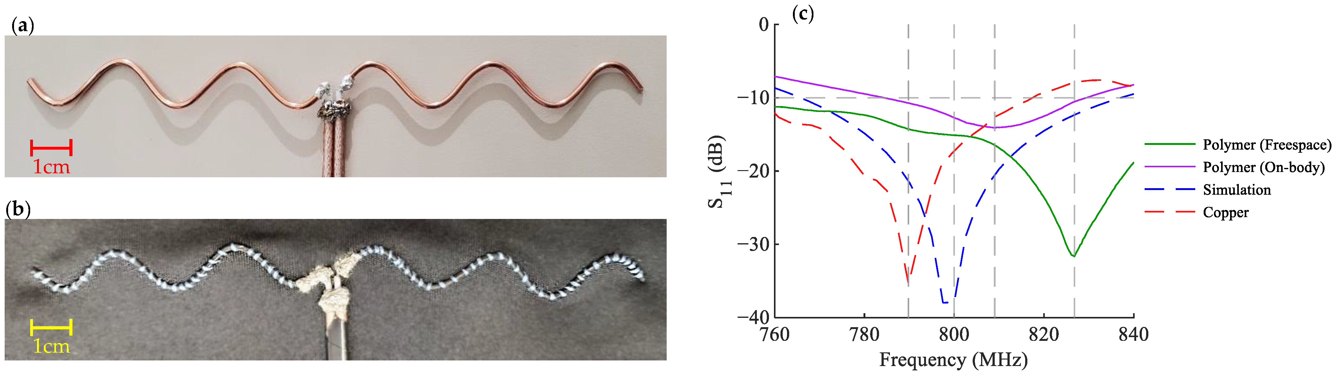
| Copper | 790 MHz | |
| Conductive Polymer (Free space) | 827 MHz | |
| Conductive Polymer (Over the Body) | 808 MHz |
| Description | Strain Type | Stretchability/Max. Bending | Sensitivity to Strain | Year | Ref. |
|---|---|---|---|---|---|
| Sinusoidal dipole antenna * | Stretching | 30% | 0.40 | 2022 | This work |
| Serpentine meshed patch over ground plane | Stretching | 40% | 0.20 | 2021 | [7] |
| Serpentine meshed in patch and ground planes | Stretching | 100% | 0.25 | 2021 | [7] |
| RFID Meandered half-wave dipole in Ecoflex | Stretching | Not provided | 0.141 ** | 2019 | Based on [8] |
| Flexible planar dipole antenna over Kepton tape | Stretching | Not provided | 0.066 ** | 2012 | Based on [42] |
| Liquid metal loop antenna | Stretching | 40% | 0.18 | 2009 | [43] |
| Graphene patch antenna over copper tape | Bending | Not provided | 1.4 | 2021 | [9] |
| Flexible multi-layer graphene film | Bending | Not provided | 5.39 | 2018 | [10] |
| Aluminum tape patch over cellulose substrate | Bending | 3.49 | 2016 | [11] |
| Description | Resonance Freq | Sensitivity to Strain (kHz/με) * | Year | Ref. |
|---|---|---|---|---|
| Double split-ring resonator (dSRR) antenna | 2.725 GHz | −1.548 | 2022 | [16] |
| Rectangular microstrip antenna | 2.725 GHz | −2.379 | 2022 | [16] |
| Rectangular microstrip antenna | 2.469 GHz | −2.847 | 2021 | [12] |
| Sierpinski fractal microstrip patch | 2.725 GHz | −1.18 | 2019 | [15] |
| Circular patch antenna | 2.5 GHz | −2.05 | 2018 | [13] |
| RFID folded patch antenna | 911.6 MHz | −0.76 | 2015 | [14] |
Publisher’s Note: MDPI stays neutral with regard to jurisdictional claims in published maps and institutional affiliations. |
© 2022 by the authors. Licensee MDPI, Basel, Switzerland. This article is an open access article distributed under the terms and conditions of the Creative Commons Attribution (CC BY) license (https://creativecommons.org/licenses/by/4.0/).
Share and Cite
Ahadi, M.; Roudjane, M.; Dugas, M.-A.; Miled, A.; Messaddeq, Y. Wearable Sensor Based on Flexible Sinusoidal Antenna for Strain Sensing Applications. Sensors 2022, 22, 4069. https://doi.org/10.3390/s22114069
Ahadi M, Roudjane M, Dugas M-A, Miled A, Messaddeq Y. Wearable Sensor Based on Flexible Sinusoidal Antenna for Strain Sensing Applications. Sensors. 2022; 22(11):4069. https://doi.org/10.3390/s22114069
Chicago/Turabian StyleAhadi, Mehran, Mourad Roudjane, Marc-André Dugas, Amine Miled, and Younès Messaddeq. 2022. "Wearable Sensor Based on Flexible Sinusoidal Antenna for Strain Sensing Applications" Sensors 22, no. 11: 4069. https://doi.org/10.3390/s22114069
APA StyleAhadi, M., Roudjane, M., Dugas, M.-A., Miled, A., & Messaddeq, Y. (2022). Wearable Sensor Based on Flexible Sinusoidal Antenna for Strain Sensing Applications. Sensors, 22(11), 4069. https://doi.org/10.3390/s22114069