Article

Blind Source Separation Based on Double-Mutant Butterfly Optimization Algorithm

1
Communication and Network Laboratory, Dalian University, Dalian 116622, China
2
National Laboratory of Radar Signal Processing, Xidian University, Xi’an 710071, China
*
Author to whom correspondence should be addressed.
Sensors 2022, 22(11), 3979; https://doi.org/10.3390/s22113979
Submission received: 2 May 2022 / Revised: 17 May 2022 / Accepted: 20 May 2022 / Published: 24 May 2022
(This article belongs to the Special Issue Artificial Intelligence-Based Audio Signal Processing)

Abstract

:
The conventional blind source separation independent component analysis method has the problem of low-separation performance. In addition, the basic butterfly optimization algorithm has the problem of insufficient search capability. In order to solve the above problems, an independent component analysis method based on the double-mutant butterfly optimization algorithm (DMBOA) is proposed in this paper. The proposed method employs the kurtosis of the signal as the objective function. By optimizing the objective function, blind source separation of the signals is realized. Based on the original butterfly optimization algorithm, DMBOA introduces dynamic transformation probability and population reconstruction mechanisms to coordinate global and local search, and when the optimization stagnates, the population is reconstructed to increase diversity and avoid falling into local optimization. The differential evolution operator is introduced to mutate at the global position update, and the sine cosine operator is introduced to mutate at the local position update, hence, enhancing the local search capability of the algorithm. To begin, 12 classical benchmark test problems were selected to evaluate the effectiveness of DMBOA. The results reveal that DMBOA outperformed the other benchmark algorithms. Following that, DMBOA was utilized for the blind source separation of mixed image and speech signals. The simulation results show that the DMBOA can realize the blind source separation of an observed signal successfully and achieve higher separation performance than the compared algorithms.

1. Introduction

Blind source separation (BSS), sometimes referred to as blind signal processing, is capable of recovering a source signal from an observed signal in the absence of critical information, such as source and channel [1,2,3]. Due to its high adaptability and other advantages, BSS has been employed in a variety of research fields in recent years, such as image processing, medical evaluation, radar analysis, speech recognition, and machinery [4,5,6,7,8].
Independent component analysis (ICA) is an important BSS method [9]. However, the conventional natural gradient algorithm (NGA) is too reliant on gradient information [10], whereas the fast fixed-point algorithm for ICA (FastICA) is sensitive to the initial solution [11]. Thus, improving the speed and precision with which the separation matrix is solved and obtaining higher-quality separated signals have significant practical implications.
To address the aforementioned issues, a swarm intelligence algorithm with a solid coevolution mechanism is gradually applied to ICA. Preliminary research indicates that BSS based on a swarm intelligence algorithm outperforms traditional BSS methods in terms of separation performance [12]. Li et al. [13] utilized the improved particle swarm optimization (PSO) for ICA. The disadvantage is the poor search capability of PSO in the later stages of iteration. Wang et al. [14] employed the improved artificial bee colony (ABC) optimization as the optimization algorithm for ICA, despite the fact that this optimization algorithm is very parameter dependent. Luo et al. [15,16] applied the improved fireworks algorithm (FA) to the radar signal processing, while the fireworks algorithm is prone to local extremum. Wen et al. [17] used a genetic algorithm (GA) to ICA, although the local search capability of GA is limited.
The butterfly optimization algorithm (BOA) was developed in 2018. It was inspired by the behavior of butterflies looking for food and demonstrated high robustness and global convergence while addressing complex optimization problems [18]. According to preliminary studies, BOA is very competitive in function optimization when compared to other metaheuristic algorithms, such as ABC, cuckoo search algorithm (CSA), firefly algorithm (FA), GA, and PSO [19]. It does, however, face several difficulties. For instance, it is possible to fall into local optimization when dealing with high-dimensional complexity prior to optimization operation. Additionally, inappropriate parameters result in a slow convergence speed of BOA. Therefore, scholars have proposed a series of improved algorithms to improve the performance of BOA. Arora et al. [20] combined BOA and ABC, enhancing the algorithm’s exploitation capacity. Long et al. [21] provided a pinhole image learning strategy based on the optical principle that can help avoid premature convergence in the algorithm. Fan et al. [22] introduced a new fragrance coefficient and a different iteration and update strategy. Mortazavi et al. [23] proposed a novel fuzzy decision strategy and introduced a notion of “virtual butterfly” to enhance the search capability of BOA. Zhang et al. [24] proposed a heuristic initialization strategy combined with greedy strategy, which improved the diversity of the initial population. Li et al. [25] introduced weight factor and Cauchy mutation to BOA, enhancing the ability of the algorithm to jump out of local optimization. The above references are some improvement methods of BOA. Although they can improve the search performance of the algorithm to some extent and reduce the premature convergence phenomenon in the algorithm, most improved algorithms only focus on the improvement of single search performance and ignore the balance between global search ability and local search ability.
Based on the foregoing research, and in response to the limitations of the low separation performance of conventional ICA methods and the lack of search ability in basic BOA, this paper presents an ICA method based on the double-mutant butterfly algorithm (DMBOA). Firstly, the dynamic transformation probability and population reconstruction mechanisms are introduced to assist the algorithm in maintaining its search balance and increasing its capacity to avoid the local optimum. The differential evolution operator is then introduced in the global position update to allow for mutation, while the sine cosine operator is introduced in the local position update to allow for mutation, hence, enhancing the algorithm’s exploitation capacity. Finally, the superiority of DMBOA is verified in benchmark function and BSS problem.
To summarize, the major contributions of this paper are given as follows:
(1)
An ICA method based on DMBOA is designed to address the low-separation performance of conventional ICA. DMBOA is used to optimize the separation matrix W, maximize the kurtosis, and finally, complete the separation of observation signals.
(2)
Three improved strategies are designed for the insufficient search capability of the basic BOA, which coordinate the global search and local search of the algorithm while improving BOA searching ability.
(3)
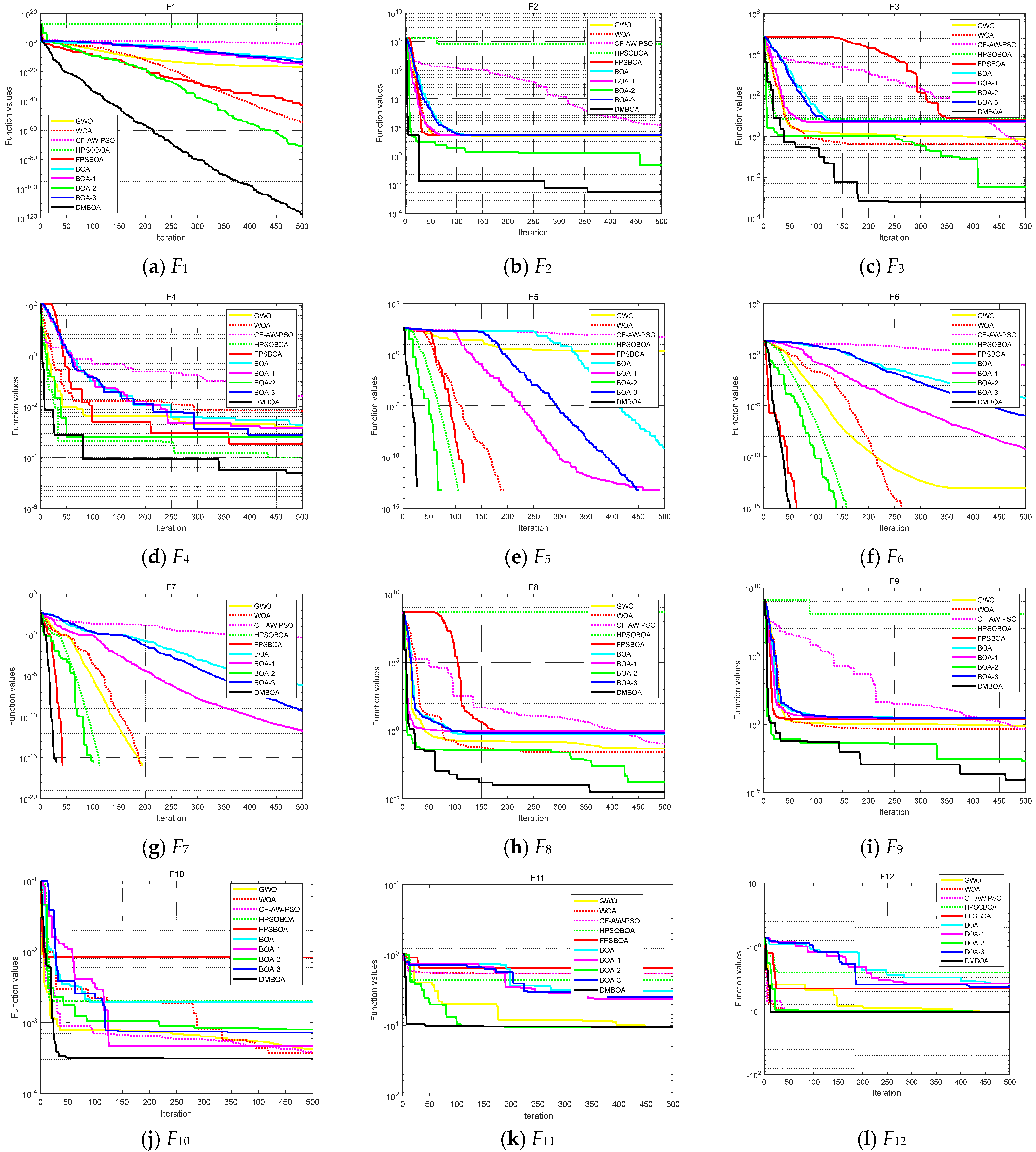
Simulation results show that DMBOA outperforms the other nine algorithms when optimizing 12 benchmark functions. In the BSS problem, DMBOA is capable of successfully separating mixed signals and achieving higher separation performance than the compared algorithms.
The remainder of this paper is organized as follows: Section 2 introduces the basic theory of BSS. Section 3 discusses the details of the BOA. Section 4 addresses the DMBOA implementation. Section 5 provides simulation analysis, which verifies the effectiveness of the proposed algorithm. Section 6 concludes the paper and summarizes the major contributions.
The main literature contributions in the introduction are introduced in Table 1.

2. Basic Theory of Blind Source Separation

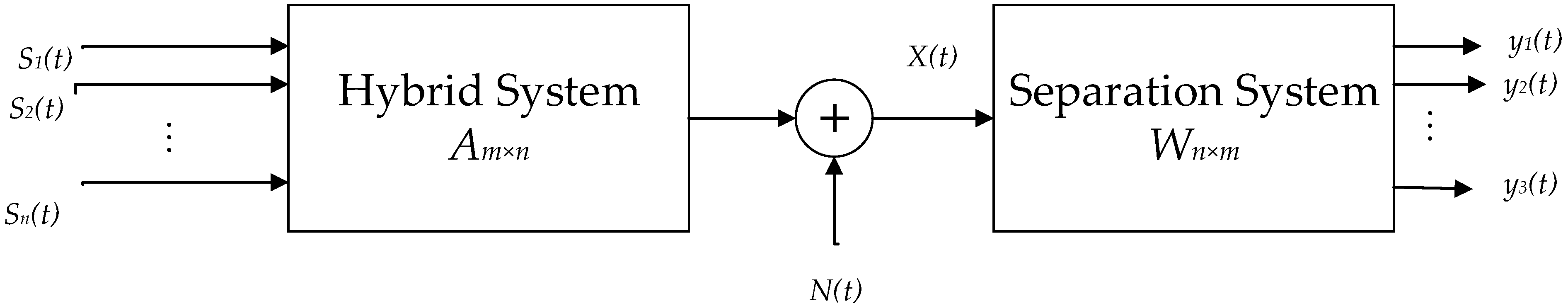
2.1. Linear Mixed Blind Source Separation Model

The linear mixed BSS model is described below:
X ( t ) = A S ( t ) + N ( t )
where t is the sampling moment, A is a mixed matrix of order m × n ( m n ), X(t) is a vector of the m-dimensional observed signals, X ( t ) = [ X 1 ( t ) , X 2 ( t ) , , X m ( t ) ] , S(t) is a vector of the n-dimensional source signals, S ( t ) = [ S 1 ( t ) , S 2 ( t ) , , S n ( t ) ] , N(t) is a vector of the m-dimensional noise signals. BSS represents the cases in which an optimization algorithm determines the separation matrix, W, when only the observed signals, X(t), are known. In such instances, the separated signals, Y(t), are obtained using Equation (2).
Y ( t ) = W X ( t )
where Y ( t ) = [ Y 1 ( t ) , Y 2 ( t ) , , Y n ( t ) ] .
To ensure the feasibility of BSS, the following assumptions are required:
(1)
The mixing matrix, A, should be reversible or full rank, and the number of observed signals should be larger than or equal to the number of source signals (i.e.,).
(2)
From a statistical standpoint, each source signal is independent of the others, and at most, one signal follows a Gaussian distribution, because multiple Gaussian processes remain a Gaussian process after mixing and, hence, cannot be separated.
Due to the lack of source signal and channel information, it is difficult to discern the signal’s amplitude and order following BSS, a phenomenon known as fuzziness. Although BSS is fuzzy, its fuzziness has a negligible effect on the results in the majority of scientific research and production practices.
Figure 1 shows the linear mixed blind source separation model.

2.2. Signal Preprocesing

Prior to performing BSS on observed signals, it is usually essential to preprocess the signals in order to simplify the separation process. De-averaging and whitening are two widely used preprocessing techniques.
The de-averaging processing method is shown in Equation (3).
X = X E ( X )
The purpose of whitening is to eliminate the signals’ correlation. The whitening operation in BSS is used to remove the second-order correlations between signals in space, ensuring that the observed signals received by the sensor remain uncorrelated in space and simplifying the algorithm complexity. The signal, V, after whitening is expressed as follows:
V = Q X = E 1 / 2 U T X
where Q is a whitening matrix, U is a characteristic matrix composed of eigenvectors corresponding to the n maximum eigenvalues of the autocorrelation matrix, R X X = E [ X X H ] , of the observed matrix, X, and E = d i a g ( d 1 , d 2 , d n ) is a diagonal matrix composed of these eigenvalues.
The separation matrix, W, is an orthogonal matrix, which can be expressed as the product of a series of rotation matrices [26]. Taking three source signals as an example, the separation matrix, W, is defined as follows:
W = [ 1 0 0 0 cos θ 1 sin θ 1 0 sin θ 1 cos θ ] [ cos θ 2 0 sin θ 2 0 1 0 sin θ 2 0 cos θ 2 ] [ cos θ 3 sin θ 3 0 sin θ 3 cos θ 3 0 0 0 1 ]

2.3. Separation Principle

When performing BSS on mixed signals using ICA, it is necessary to first select an appropriate criterion for determining the statistical independence of the separated signals. Afterwards, the objective function is established and optimized using the appropriate algorithm. This leads to the separation matrix with the strongest independence of the separated signals.
The commonly used independence criterion of signals includes mutual information, kurtosis, and negative entropy. Kurtosis is calculated using Equation (6) as follows:
K ( y i ) = k u r t ( y i ) = E { y i 4 } 3 ( E { y i 2 } 2 )
where yi is a gaussian random variable.
The sum of absolute values of kurtosis is used as a criterion of signal independence in this paper, and the objective function is specified as follows:
f i t i = 1 i = 1 n | K ( y i ) | + ε
where ε is an extremely small amount that prevents division by zero. According to the information theory, for a gaussian random vector yi, when E [ y y T ] = I , the larger the kurtosis of the signals, the greater their independence. The above-mentioned DMBOA will be used to optimize the separation matrix W, to maximize the kurtosis, and finally complete the separation of the observed signals.

3. Butterfly Optimization Algorithm (BOA)

BOA is an optimization technique inspired by the foraging behavior of butterflies. Each butterfly in BOA serves as a search operator and performs the optimization process in the search space. Butterflies are capable of perceiving and distinguishing between different fragrance intensities, and each butterfly emits a fragrance of a certain intensity. Assume that the intensity of the fragrance produced by butterflies is proportional to their fitness; that is, as butterflies move from one location to another, their fitness will change accordingly. When a butterfly detects the fragrance of another, it will move toward the butterfly with the strongest fragrance. This stage is referred to as “global search.” On the contrary, if the butterfly is unable to perceive the fragrance of other butterflies, it will move randomly. This stage is referred to as “local search.” The global and local searches are switched during the search process by switching the probability p.
The fragrance can be formulated as follows:
f = c I a
where f is the perceived intensity of the fragrance, i.e., the fragrance’s intensity as perceived by other butterflies, c is the sensory modality, I is the stimulus intensity, depending on fitness, and a is the mode-dependent power exponent, which accounts for the various degrees of absorption, a [ 0 , 1 ] . The value of c is updated by Equation (9) as follows:
c t + 1 = c t + 0.025 / ( c t × T )
where t and T represent the current and maximum number of iterations, respectively.
When butterflies sense the stronger fragrance in the area, they move towards the strongest one. This stage is calculated as follows:
x i t + 1 = x i t + ( r 2 × g x i t ) × f
When a butterfly is unable to perceive the surrounding fragrance, it moves randomly. This stage is calculated as follows:
x i t + 1 = x i t + ( r 2 × x j t x k t ) × f
where x i t represents the position of butterfly individual i in generation t, x j t denotes the position of butterfly individual j in generation t, x k t indicates the position of butterfly individual k in generation t, r shows a random number between 0 and 1, and g stands for the gl obal optimal position.
The pseudo code of BOA is provided in Algorithm 1.
Algorithm 1: BOA
Input: Objective function f(x), butterfly population size N, stimulation concentration I, sensory modality c = 0.01 , power exponent a = 0.1 , conversion probability p = 0.8 , Maximum number of iterations T.
1. Initialize population
2. While t < T
3.   for i = 1: N
4.   Calculate fragrance using Equation (8)
5.   Generate a random number rand in [0, 1]
6.   if  rand < p
7.     Update position using Equation (10)
8.   else
9.     Update position using Equation (11)
10.    end if
11.    if f ( x i t ) f ( g )
12.       g = x i t , f ( g ) = f ( x i t )
13.    end if
14.    Update the value of c using Equation (9)
15. end for
16. end while
17. Output the global optimal solution

4. Double-Mutant Butterfly Optimization Algorithm (DMBOA)

4.1. Dynamic Transition Probability

Local and global searches are controlled in the basic BOA by the constant switching probability p, which implies that during the iterative process of the algorithm, BOA will allocate 80% of its search capability to global search and 20% to local search. In this search mode, about 80% of the butterflies in the population will be attracted to the best butterfly, g. Therefore, if the best butterfly, g, falls into the local optimum, it will strongly guide other butterflies to this unpopular position in the search space, making it more difficult for the algorithm to avoid the local extreme value, so it converges prematurely.
A reasonable search process should begin with a strong global search in the early stages of the algorithm, quickly locate the scope of the global optimal solution in the search space, and appropriately enhance the local development capability in the latter stages of the exploration, all of which contribute to the optimization accuracy of the algorithm. The dynamic switching probability, p2, is proposed in this paper to balance the proportions of local and global search to achieve a more effective optimization strategy. The dynamic conversion probability, p2, is shown in Equation (12).
p 2 = 0.8 0.3 × sin ( π μ ( t T ) 2 )
where μ takes constant 2.
As seen in Figure 2, the dynamic conversion probability, p2, proposed in this paper, gradually converges to 0.5 as iteration progresses. It can strike a balance between global search in the early stages and local development in the latter stages.

4.2. Improvement in Update Function

When some butterflies move completely at will or when a large number of butterflies congregate at non-global extreme points, the convergence speed of BOA is significantly slowed and falls into local extreme values. Two mutation operators, the differential evolution [27,28] and sine cosine operator [29], are used in this paper to improve BOA.
The differential evolution operator utilizes three-parameter variables for global search, which results in a faster convergence rate and simplifies the process of obtaining the global optimal value, which is why it is used for global search. The sine cosine operator possesses the periodicity and oscillation of the sine cosine function, which enables it to avoid falling into the local extremum, accelerate the convergence speed of the algorithm, and be applied to local search.
The global search variation is expressed as follows:
x i t + 1 = x i t × r 1 + F × [ λ × ( g x j t ) ( 1 λ ) × ( g x k t ) ]
The local search variation is determined as follows:
x i t + 1 = { x i t × sin r 2 + ( 1 r 1 ) × | r 3 × g x i t | r 4 < 0.5 x i t × cos r 2 + ( 1 r 1 ) × | r 3 × g x i t | r 4 0.5
where the mutation operator, F [ 0 , 2 ] , is a real constant factor, r 2 is a random number with a value range between 0 and 2π, and λ and r3 are random numbers with a value range between 0 and 1. The parameter r1 is calculated as follows:
r 1 = δ t × δ T
where δ takes constant 2.

4.3. Population Reconstruction Mechanism

The counter count is introduced, with an initial value of 0. If the global optimal solution, g, remains constant, the count increases by 1. If the global optimal solution, g, changes, the counter is reset. When the count is greater than or equal to 0.1 T , the default optimization stops. To preserve previous optimization results and increase the population diversity to avoid local optimums, 20% of the individuals, including the optimal solution, are randomly selected from the original population, while the remaining 80% of individuals are discarded and replaced with new randomly generated individuals.
Algorithm 2 gives the pseudo code of DMBOA, and Figure 3 shows the flow chart of DMBOA-ICA.
Algorithm 2: DMBOA
Input: Objective function f(x), butterfly population size N, stimulation concentration I, sensory modality c = 0.01 , power exponent a = 0.1 , maximum number of iterations T.
counter c o u n t = 0 .
1. Initialize population
2. Whilet < T
3.   for i = 1: N
4.    Calculate fragrance using Equation (8)
5.    Calculate conversion probability p using Equation (8)
6.    Generate a random numbers rand in [0, 1]
7.      if  rand < p
8.      Update position using Equation (13)
9.     else
10.       Update position using Equation (14)
11.   end if
12.   if f ( x i t ) f ( g )
13.      g = x i t , f ( g ) = f ( x i t ) , c o u n t = 0
14.   else
15.         c o u n t = c o u n t + 1
16.   end if
17.   if c o u n t 0.1 T
18.       Execute population reconstruction strategy
19.   end if
20.   Update the value of c using Equation (9)
21.   end for
22. end while
23. Output the global optimal solution
The DMBOA proposed in this paper enhances the basic BOA in three aspects. Firstly, the dynamic transformation probability coordination algorithm is implemented using both local and global search. The double-mutant operator is then incorporated into the algorithm update function to enhance the local search capability of the algorithm. Finally, a population reconstruction mechanism is introduced to avoid falling into local optimums in the event of optimization stagnation. Through the above three improvement methods, DMBOA can effectively overcome the poor search capability of the basic BOA, which makes it easy to fall into local optimums. However, when compared to the basic BOA, DMBOA has a higher computational complexity, as each iteration of DMBOA requires calculating the value of the calculator count and reconstructing the population when it falls into optimization stagnation, which, in turn, increases the calculations required by this algorithm.

5. Simulation and Result Analysis

5.1. Evalution of DMBOA on Benchmark Function

To more accurately and comprehensively verify the efficacy of DMBOA, 12 test functions were used with varying characteristics for experiments. The detailed characteristics of each test function are listed in Table 2. It features four single-mode test functions (F1–F4), as well as eight multi-mode test functions (F5–F12). In Table 2, Dim denotes the function dimension, Scope represents the value range of x, and fmin indicates the ideal value of each function. There is only one global optimal solution for single-mode test functions and no local optimal solution. They are suitable for evaluating the local development capability of the algorithm. On the contrary, there are many local optimal solutions for multimodal test functions. Numerous algorithms that perform well with low modal functions perform poorly with high modal functions and are prone to local optimization or oscillation between local extrema. The high-modal test function is usually used to evaluate the global search capability of the algorithm [30].
DMBOA is compared against nine algorithms in the experiment, namely GWO [31], WOA [32], CF-AW-PSO [33], HPSOBOA [34], FPSBOA [35], BOA [18], BOA_1 (dynamic conversion probability), BOA_2 (introduce double-mutant operator), and BOA_3 (introduce population reconstruction mechanism). For all ten algorithms, the population size N = 30 and the total number of iterations T = 500. The parameters of DMBOA are shown in Algorithm 2, while the parameters of other algorithms are shown in references [31,32,33,34,35]. Table 2 shows the optimal fitness value (BEST), the average fitness value (MEAN), the standard deviation (STD), and the running time (TIME), tested by 10 algorithms, such as DMBOA under 12 test functions in Table 2, in which the time unit is seconds. The test results of DMBOA have been bold in Table 3. Each algorithm was performed separately 30 times to minimize the error, and all experiments were conducted on a laptop equipped with an Intel (R) Core (TM) i7-6500 CPU at 2.50 GHz and 8 GB of RAM.
As shown in Table 3, DMBOA is capable of obtaining the optimal values for these 12 test functions, and the optimal values for each function are closer to fmin in Table 2. The search accuracy of BOA_1, BOA_2, and BOA_3 proposed in this paper is also better than the original BOA, demonstrating the efficacy of the three improvement strategies utilized in this paper. DMBOA has a higher search accuracy than the improved algorithm with a single strategy, indicating that under the joint influence of different strategies, the optimization ability and stability of the algorithm are improved to the greatest extent. Overall, the test results of BOA_2 are closer to those of DMBOA. The STD of data can reflect the degree of dispersion. According to the test results in Table 3, DMBOA has the smallest STD for each test function, indicating that it is more robust and stable than the compared algorithms when dealing with both low- and high-modal problems. As for the calculation time in Table 3, DMBOA has a medium execution time. According to the data in the table, the test time for DMBOA under the five test functions of F2, F4, F5, F11, and F12 is less than that of the original BOA. This indicates that, although the time complexity of DMBOA is higher in theory than that of the original BOA, the high convergence accuracy of DMBOA enables it to find the global optimal solution more quickly, particularly for the two test functions, F11 and F12.
Figure 4 depicts the iteration history of the ten algorithms tested on the 12 test functions in Table 2. As seen in Figure 4, the DMBOA developed in this study has the fastest iteration speed and maximum convergence accuracy among all the convergence history graphs. This demonstrates that, when compared to other algorithms, DMBOA is capable of obtaining the optimal solution in the shortest amount of time. BOA-1, BOA-2, and BOA-3, which are improved by a single strategy, improved convergence speed and optimization accuracy to a certain extent when compared to basic BOA, indicating that each strategy performed satisfactorily and effectively, but not as well as the DMBOA, which is improved by a hybrid strategy. The feasibility of the three improved strategies is further verified. GWO can be iterated until it reaches the theoretical optimal value under F5 and F7. The overall convergence performance of WOA is general. The convergence speed of CF-AW-PSO is slow in the early stages. The iteration results of HPSOBOA under F1, F2, F6, and F7 are poor. FPSBOA outperforms F5, F6, and F7 in terms of convergence curve and search performance.

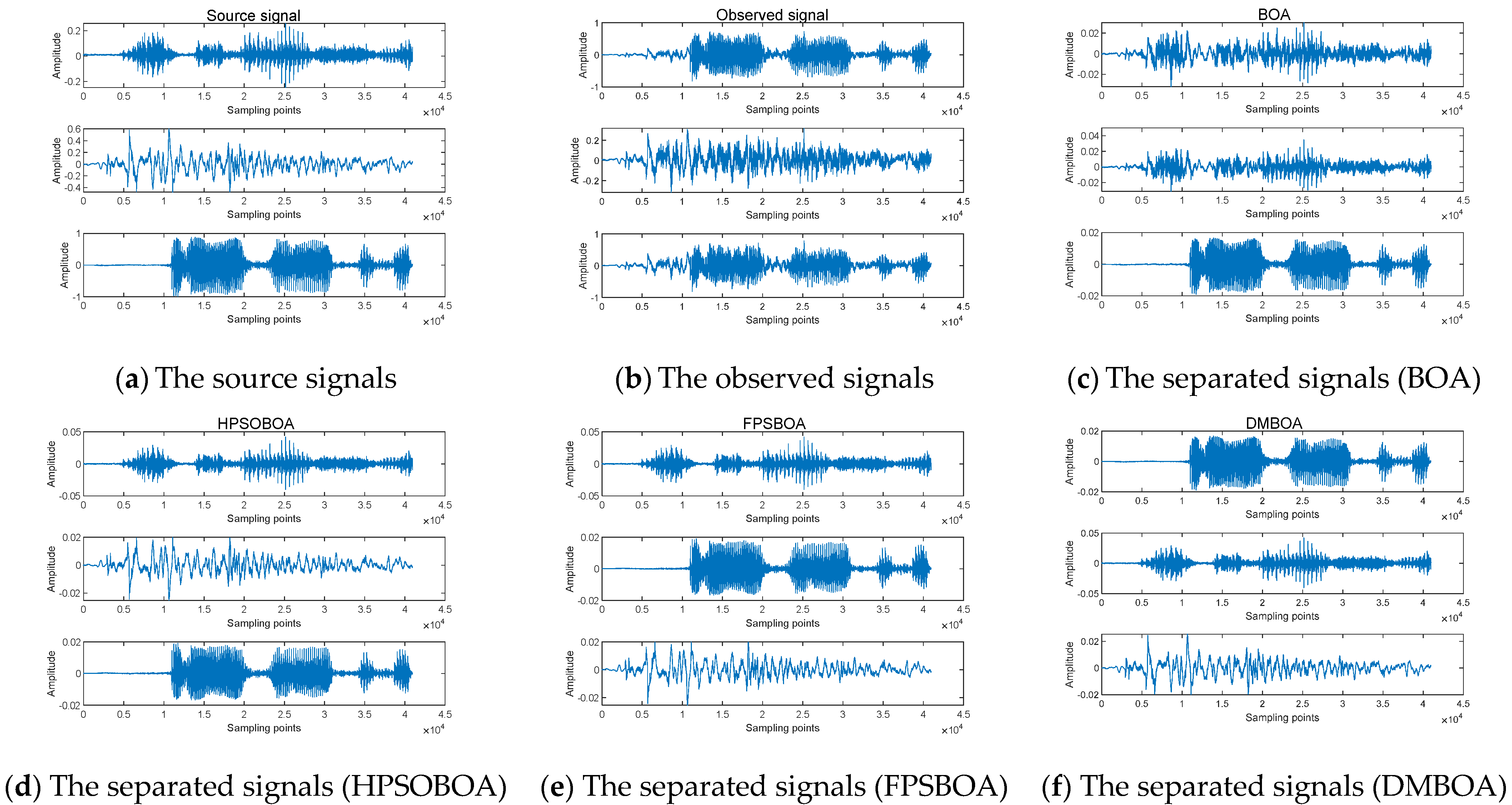
5.2. Speech Signal Separation

Three speech signals are used as the source signals, which are then mixed to obtain the observed signals. To acquire the separated signals, DMBOA, BOA, HPSOBOA, and FPSBOA are used to blindly separate the observed signals. The simulation diagram is depicted in Figure 5. The sampling frequency and sampling point of voice signals are 40,964 and 1000, respectively.
In order to quantitatively analyze and compare the separation performance of the four algorithms, the time, similarity coefficient, performance index (PI), and PESQ [36] are employed in this study. The data are shown in Table 4 with a time unit of seconds.
The PESQ metric is based on the wide-band version recommended in ITU-T [37], and its range is extended from −0.5 to 4.5. The higher its value, the better the quality of the speech signal. The similarity coefficient and PI are expressed in Equations (16) and (17) as follows:
ρ i j = | i = 1 N s i ( t ) y j ( t ) | i = 1 N s i 2 ( t ) t = 1 N y j 2 ( t )
P I = 1 N ( N 1 ) i = 1 N { ( i = 1 N | G i j | max i | G i l | 1 ) + ( j = 1 N ( | G i j | max j | G i l | 1 ) }
In Equation (16), ρ i j is a similarity index used to compare the source signal with the separated signal. The greater the ρ i j , the more effective the separation. In this section, ρ i j is a 3 × 3 matrix. The maximum value of each channel is taken as the experimental data, and N is set to 3. Additionally, in Equation (17),
; the closer the PI is to 0, the more similar the separated signal is to the source signal.
In comparison to Figure 5, the separated signals have a different amplitude and order than the source signals, indicating the fuzziness of BSS. The signals separated by BOA are partially distorted. The signals separated by HPSOBOA and FPSBOA are partially deformed. The signals separated by DMBOA are highly consistent with the waveform of the source signal and have a strong separation effect.
As shown in Table 4, DMBOA produces not only the highest similarity coefficient and PESQ but also the smallest PI of the separated signal, allowing for a more accurate restoration of the source signal. Moreover, the operation time of DMBOA is shorter than that of the examined algorithms.

5.3. Image Signal Separation

Three gray-scale images and one random noise image are used as source signals, and they are combined to produce the observed signals. To acquire the separated signals, DMBOA, BOA, HPSOBOA, and FPSBOA are used to blindly separate the observed signals. In this section, N is assumed to be 4, and the pixels of the image are 256 × 256 ; ρ i j is a 4 × 4 matrix. Figure 6 illustrates the simulation result and Table 5 compares the similarity coefficient, PI, and duration of separated signals, as well as the SSIM [38] of the output image. The SSIM proves to be a better error metric for comparing the image quality with better structure preservation. They are in the range of [0, 1], which is a value closer to one indicating better structure preservation:
SSIM = ( 2 μ x ^ μ x + C 1 ) ( 2 σ x ^ x + C 2 ) ( μ x ^ 2 + μ x 2 + C 1 ) ( σ x ^ 2 + σ x 2 + C 2 )
where C 1 and C 2 are constant, σ x ^ x represents the covariance of image, μ x ^ and μ x represent the mean value of the two images, respectively, σ x ^ and σ x represent the variance in the two images, respectively.
As seen in Figure 6, the images separated by DMBOA are similar to the source images, but the images separated by other algorithms have varying degrees of ambiguity. Additionally, as demonstrated by the data in Table 5, the separation performance of DMBOA is superior to that of the examined algorithms.

6. Conclusions

This paper proposed a novel double-mutant butterfly optimization algorithm (DMBOA), which is a major improvement on the butterfly optimization algorithm (BOA) and applied to blind source separation (BBS). The algorithm incorporates a double-mutant operator and a population reconstruction mechanism, which enhances the capability of local development and avoids local optimization. The proposed technique was initially explored and further developed through the use of a dynamic conversion probability balancing method. The following conclusions are drawn from the simulation results:
(1)
When optimizing 12 benchmark functions (four low-modal and eight high-modal), DMBOA outperforms the other nine algorithms. The three improvement methods proposed in this study increased the performance of BOA to varying degrees in the algorithm ablation experiment. All of this demonstrates that DMBOA has a high level of search performance and strong robustness.
(2)
DMBOA outperforms the other algorithms in the BSS and is capable of successfully separating the mixed speech and image signals.

Author Contributions

Conceptualization, Q.X. and Y.D.; Data curation, Q.X., H.Z. and X.D.; Formal analysis, Q.X. and Y.D.; Funding acquisition, Y.D.; Investigation, Q.X.; Methodology, Q.X.; Project administration, Y.D.; Resources, Y.D. and R.Z.; Software, Q.X.; Supervision, Y.D. and R.Z.; Validation, Q.X., Y.D. and M.L.; Visualization, Q.X.; Writing—original draft, Q.X.; Writing—review and editing, Q.X., Y.D., R.Z. and M.L. All authors have read and agreed to the published version of the manuscript.

Funding

This research was funded by the National Natural Science Foundation of China and General Project Fund in the Field of Equipment Development Department, grant number (No. 61901079, No. 61403110308). The APC was funded by Dalian University.

Institutional Review Board Statement

Not applicable.

Informed Consent Statement

Not applicable.

Data Availability Statement

Not applicable.

Conflicts of Interest

The authors declare no conflict of interest.

References

  1. Gao, J.; Zhu, X.; Nandi, A. Independent Component Analysis for Multiple-Input Multiple-Output Wireless Communication Systems. Signal Processing 2011, 91, 607–623. [Google Scholar] [CrossRef]
  2. Cheng, Y.; Zhu, D.; Zhang, J. High Precision Sparse Reconstruction Scheme for Multiple Radar Mainlobe Jammings. Electronics 2020, 9, 1224. [Google Scholar] [CrossRef]
  3. Zi, J.; Lv, D.; Liu, J.; Huang, X.; Yao, W.; Gao, M.; Xi, R.; Zhang, Y. Improved Swarm Intelligent Blind Source Separation Based on Signal Cross-Correlation. Sensors 2022, 22, 118. [Google Scholar] [CrossRef] [PubMed]
  4. Ali, K.; Nourredine, A.; Elhadi, K. Blind Image Separation Using the JADE Method. Eng. Proc. 2022, 14, 20. [Google Scholar]
  5. Taha, L.; Abdel-Raheem, E. A Null Space-Based Blind Source Separation for Fetal Electrocardiogram Signals. Sensors 2020, 20, 3536. [Google Scholar] [CrossRef]
  6. Xu, H.; Ebrahim, M.P.; Hasan, K.; Heydari, F.; Howley, P.; Yuce, M.R. Accurate Heart Rate and Respiration Rate Detection Based on a Higher-Order Harmonics Peak Selection Method Using Radar Non-Contact Sensors. Sensors 2022, 22, 83. [Google Scholar] [CrossRef]
  7. Guo, S.; Shi, M.; Zhou, Y.; Yu, J.; Wang, E. An Efficient Convolutional Blind Source Separation Algorithm for Speech Signals under Chaotic Masking. Algorithms 2021, 14, 165. [Google Scholar] [CrossRef]
  8. Ding, H.; Wang, Y.; Yang, Z.; Pfeiffer, O. Nonlinear Blind Source Separation and Fault Feature Extraction Method for Mining Machine Diagnosis. Appl. Sci. 2019, 9, 1852. [Google Scholar] [CrossRef]
  9. Comon, P. Independent Component Analysis, A New Concept? Signal Processing 1994, 36, 287–314. [Google Scholar] [CrossRef]
  10. Amari, S. Natural Gradient Works Efficiently in Learning. Neural Comput. 1998, 10, 251–276. [Google Scholar] [CrossRef]
  11. Barros, A.; Cichocki, A. A Fixed-Point Algorithm for Independent Component Analysis which Uses A Priori Information. In Proceedings of the 5th Brazilian Symposium on Neural Networks, Belo Horizonte, Brazil, 9–11 December 1998. [Google Scholar]
  12. Lee, S.; Yang, C. GPSO-ICA: Independent Component Analysis Based on Gravitational Particle Swarm Optimization for Blind Source Separation. J. Intell. Fuzzy Syst. 2018, 35, 1943–1957. [Google Scholar] [CrossRef]
  13. Li, C.; Jiang, Y.; Liu, F.; Xiang, Y. Blind Source Separation Algorithm Based on Improved Particle Swarm Optimization under Noisy Condition. In Proceedings of the 2018 2nd IEEE Advanced Information Management, Communicates, Electronic and Automation Control Conference, Xian, China, 25–27 May 2018. [Google Scholar]
  14. Wang, R. Blind Source Separation Based on Adaptive Artificial Bee Colony Optimization and Kurtosis. Circuits Syst. Signal Processing 2021, 40, 3338–3354. [Google Scholar] [CrossRef]
  15. Luo, W.; Jin, H.; Li, H.; Fang, X.; Zhou, R. Optimal Performance and Application for Firework Algorithm Using a Novel Chaotic Approach. IEEE Access 2020, 8, 120798–120817. [Google Scholar] [CrossRef]
  16. Luo, W.; Jin, H.; Li, H.; Duan, K. Radar Main-Lobe Jamming Suppression Based on Adaptive Opposite Fireworks Algorithm. IEEE Open J. Antennas Propag. 2021, 2, 138–150. [Google Scholar] [CrossRef]
  17. Wen, G.; Zhang, C.; Lin, Z.; Shang, Z.; Wang, H.; Zhang, Q. Independent Component Analysis Based on Genetic Algorithms. In Proceedings of the 2014 10th International Conference on Natural Computation, Xiamen, China, 19–21 August 2014. [Google Scholar]
  18. Arora, S.; Singh, S. Butterfly Optimization Algorithm: A Novel Approach for Global Optimization. Soft Comput. 2019, 23, 715–734. [Google Scholar] [CrossRef]
  19. Long, W.; Wu, T.; Xu, M.; Tang, M.; Cai, S. Parameters Identification of Photovoltaic Models by Using An Enhanced Adaptive Butterfly Optimization Algorithm. Energy 2021, 103, 120750. [Google Scholar] [CrossRef]
  20. Arora, S.; Singh, S. An Effective Hybrid Butterfly Optimization Algorithm with Artificial Bee Colony for Numerical Optimization. Int. J. Interact. Multimed. Artif. Intell. 2017, 4, 14–21. [Google Scholar] [CrossRef]
  21. Long, W.; Jiao, J.; Liang, X.; Wu, T.; Xu, M.; Cai, S. Pinhole-Imaging-Based Learning Butterfly Optimization Algorithm for Global Optimization and Feature Selection. Appl. Soft Comput. 2021, 103, 107146. [Google Scholar] [CrossRef]
  22. Fan, Y.; Shao, J.; Sun, G.; Shao, X. A Self-Adaption Butterfly Optimization Algorithm for Numerical Optimization Problems. IEEE Access 2020, 8, 88026–88041. [Google Scholar] [CrossRef]
  23. Mortazavi, A.; Moloodpoor, M. Enhanced Butterfly Optimization Algorithm with A New Fuzzy Regulator Strategy and Virtual Butterfly Concept. Knowl. -Based Syst. 2021, 228, 107291. [Google Scholar] [CrossRef]
  24. Zhang, B.; Yang, X.; Hu, B.; Liu, Z.; Li, Z. OEbBOA: A Novel Improved Binary Butterfly Opmization Approaches With Various Strategies for Feature Selection. IEEE Access 2020, 8, 67799–67812. [Google Scholar] [CrossRef]
  25. Li, G.; Chang, W.; Yang, H. A Novel Combined Prediction Model for Monthly Mean Precipitation With Error Correction Strategy. IEEE Access 2020, 8, 141432–141445. [Google Scholar] [CrossRef]
  26. Watkins, D. Fundamentals of Matrix Computations, 2nd ed; Wiley: New York, NY, USA, 2002; pp. 192–194. [Google Scholar]
  27. Storn, R.; Price, K. Differential Evolution–A Simple and Efficient Heuristic for global Optimization over Continuous Spaces. J. Glob. Optim. 1997, 11, 341–359. [Google Scholar] [CrossRef]
  28. Price, K. Differential Evolution: A Fast and Simple Numerical Optimizer. In Proceedings of the North American Fuzzy Information Processing, Berkeley, CA, USA, 19–22 June 1996; pp. 524–527. [Google Scholar]
  29. Mirjalili, S. SCA: A Sine Cosine Algorithm for Solving Optimization Problems. Knowl.-Based Syst. 2016, 96, 120–133. [Google Scholar] [CrossRef]
  30. Li, Y.; Ni, Z.; Jin, Z.; Li, J.; Li, F. Research on Clustering Method of Improved Glowworm Algorithm Based on Good-Point Set. Math. Probl. Eng. 2018, 2018, 8274084. [Google Scholar] [CrossRef]
  31. Mirjalili, S.; Mirjalili, S.M.; Lewis, A. Grey Wolf Optimizer. Adv. Eng. Softw. 2014, 69, 46–61. [Google Scholar] [CrossRef]
  32. Mirjalili, S.; Lewis, A. The Whale Optimization Algorithm. Adv. Eng. Softw. 2016, 95, 51–67. [Google Scholar] [CrossRef]
  33. You, Z.; Chen, W.; He, G.; Nan, X. Adaptive Weight Particle Swarm Optimization Algorithm with Constriction Factor. In Proceedings of the 2010 International Conference of Information Science and Management Engineering, Xi’an, China, 7–8 August 2010. [Google Scholar]
  34. Zhang, M.; Long, D.; Qin, T.; Yang, J. A Chaotic Hybrid Butterfly Optimization Algorithm with Particle Swarm Optimization for High-Dimensional Optimization Problems. Symmetry 2020, 12, 1800. [Google Scholar] [CrossRef]
  35. Li, Y.; Yu, X.; Liu, J. Enhanced Butterfly Optimization Algorithm for Large-Scale Optimization Problems. J. Bionic Eng. 2022, 19, 554–570. [Google Scholar] [CrossRef]
  36. Ali, M.N.; Falavigna, D.; Brutti, A. Time-Domain Joint Training Strategies of Speech Enhancement and Intent Classification Neural Models. Sensors 2022, 22, 374. [Google Scholar] [CrossRef]
  37. Fu, S.; Liao, C.; Tsao, Y. Learning with learned loss function: Speech enhancement with quality-net to improve perceptual evaluation of speech quality. IEEE Signal Process. Lett. 2019, 27, 26–30. [Google Scholar] [CrossRef]
  38. Mahdaoui, A.E.; Ouahabi, A.; Moulay, M.S. Image Denoising Using a Compressive Sensing Approach Based on Regularization Constraints. Sensors 2022, 22, 2199. [Google Scholar] [CrossRef] [PubMed]
Figure 1. Linear mixed blind source separation model.
Sensors 22 03979 g001
Figure 2. Iterative curve of transformation probability p.
Sensors 22 03979 g002
Figure 3. The flow chart of DMBOA-ICA.
Sensors 22 03979 g003
Figure 4. Convergence curves of 10 algorithms on 12 test function in Table 2.
Sensors 22 03979 g004
Figure 5. Effect drawing of speech signal separation. (a) The waveform of source signals; (b) the waveform of observed signals; (c) The waveform of BOA separated signals; (d) The waveform of HPSOBOA separated signals; (e) The waveform of FPSBOA separated signals; (f) The waveform of DMBOA separated signals.
Sensors 22 03979 g005
Figure 6. Effect drawing of image signal separation. (a) The image of source signals; (b) The image of observed signals; (c) The image of BOA separated signals; (d) The image of HPSOBOA separated signals; (e) The image of FPSBOA separated signals; (f) The image of DMBOA separated signals.
Sensors 22 03979 g006aSensors 22 03979 g006b
Table 1. The main literature contributions.
Algorithm TypeNameMethodConclusionReference
Conventional ICA NGABased on gradient informationThe separation performance of conventional algorithms is low and need to be further improved.Amari [10]
FastICABased on fixed point iterationBarros et al. [11]
Intelligent optimization ICAPSO-ICAIntroduce PSO into ICAIntroducing swarm intelligence algorithms into ICA improves the separation performance compared with conventional ICA. But there are problems with these swarm intelligence algorithms.Li et al. [13]
ABC-ICAIntroduce ABC into ICAWang et al. [14]
FA-ICAIntroduce FA into ICALuo et al. [15,16]
GA-ICAIntroduce GA into ICAWen et al. [17]
Improved algorithms of BOABOA/ABCCombines BOA and ABCMost improved algorithms only improve the single search performance of BOA, but ignore the balance between global search ability and local search ability.Arora et al. [20]
PIL-BOAProvides a pinhole image learning strategy based on the optical principleLong et al. [21]
SABOAIntroduces a new fragrance coefficient and a different iteration strategyFan et al. [22]
FBOAProposes a novel fuzzy decision strategy and introduces a notion of “virtual butterfly”Mortazavi et al. [23]
OEbBOAProposes a heuristic initialization strategy combined with greedy strategyZhang et al. [24]
IBOAIntroduces weight factor and Cauchy mutationLi et al. [25]
Table 2. Basic information of benchmark functions.
FunctionDimScopefmin
F 1 ( x ) = i = 1 n | x i | + i = 1 n | x i | 30[–10, 10]0
F 2 ( x ) = i = 1 n [ 100 ( x i + 1 x i 2 ) 2 + ( x i 1 ) 2 ] 30[−30, 30]0
F 3 ( x ) = i = 1 n ( [ x i + 0.5 ] ) 2 30[−100, 100]0
F 4 ( x ) = i = 1 n i x i 4 + random [ 0 , 1 ) 30[−1.28, 1.28]0
F 5 ( x ) = i = 1 n [ x i 2 10 cos ( 2 π x i + 10 ) ] 30[−5.12, 5.12]0
F 6 ( x ) = 20 exp ( 0.2 1 n i = 1 n x i 2 ) exp ( 1 n i = 1 n cos ( 2 π x i ) ) + 20 + e 30[−32, 32]0
F 7 ( x ) = 1 4000 i = 1 n x i 2 i = 1 n cos ( x i i ) + 1 30[−600, 600]0
F 8 ( x ) = π n { 10 sin ( π y 1 ) + i = 1 n ( y i 1 ) 2 [ 1 + 10 sin 2 ( π y i + 1 ) ] + ( y n 1 ) 2 } + i = 1 n u ( x i , 10 , 100 , 4 ) , y i = 1 + x i + 1 4 u ( x i , a , k , m ) = { k ( x i a ) m x i > a 0 a < x i < a k ( x i a ) m x i < a 30[−50, 50]0
F 9 ( x ) = 0.1 { sin 2 ( 3 π x i ) + i = 1 n ( x i 1 ) 2 [ 1 + sin 2 ( 3 π x i + 1 ) ] + ( x n 1 ) 2 [ 1 + sin 2 ( 2 π x n ) ] } + i = 1 n u ( x i , 5 , 100 , 4 ) 30[−50,50]0
F 10 ( x ) = i = 1 11 [ a i x 1 ( b i 2 + b i x 2 ) b i 2 + b i x 3 + x 4 ] 4[−5, 5]0.00030
F 11 ( x ) = i = 1 7 [ ( X a i ) ( X a i ) T + c i ] 1 4[0, 10]−10.4028
F 12 ( x ) = i = 1 10 [ ( X a i ) ( X a i ) T + c i ] 1 4[0, 10]−10.5363
Table 3. Comparative analysis of performance of 10 swarm intelligence algorithms.
FunctionIndexDMBOABOABOA_1BOA_2BOA_3HPSOBOAFPSBOAGWOWOACF_AW_PSO
F1BEST1.28 × 10−1192.75 × 10−112.42 × 10−141.13 × 10−623.01 × 10−133.19 × 10119.73 × 10−511.20 × 10−169.40 × 10−530.12256
MEAN2.04 × 1059.01 × 1073.51 × 1078.52 × 1054.71 × 1074.58 × 10132.43 × 1087.29 × 1088.05 × 1091.40 × 1012
STD2.47 × 1052.01 × 1097.47 × 1077.85 × 1077.85 × 1081.61 × 10141.68 × 1091.63 × 1098.84 × 1092.04 × 1012
TIME0.16100.15270.15430.17710.17320.17570.13750.19270.09011.0270
F2BEST1.06 × 10−228.947128.88180.178628.07152.41 × 1082.89 × 10126.876927.67662.03 × 102
MEAN1.24 × 1052.91 × 1062.51 × 1061.39 × 1062.47 × 1062.44 × 1081.32 × 1061.89 × 1061.97 × 1061.62 × 106
STD1.63 × 1062.67 × 1071.68 × 1071.68 × 1072.04 × 1079.84 × 1061.58 × 1071.80 × 1071.93 × 1071.32 × 107
TIME0.19410.20770.18440.18440.22900.19470.18840.20500.07940.9862
F3BEST1.28 × 10−35.12594.7380.00984.99926.35844.88110.62590.41280.3316
MEAN2.87 × 1022.32 × 1032.01 × 1033.30 × 1022.04 × 1032.66 × 1022.91 × 1036.50 × 1026.24 × 1021.94 × 103
STD4.02 × 1038.84 × 1037.43 × 1034.48 × 1039.00 × 1033.46 × 1037.78 × 1034.68 × 1035.10 × 1034.42 × 103
TIME0.13560.12410.13160.14780.15240.13690.12790.17740.06310.9525
F4BEST7.93 × 10−50.00208.33 × 10−46.09 × 10−41.30 × 10−31.09 × 10−45.31 × 10−41.44 × 10−30.00490.0485
MEAN0.43273.44882.35771.21251.47120.54873.69510.79351.01800.9897
STD5.164614.758011.739410.044114.92665.976815.2777.24828.15467.1023
TIME0.32570.33120.30170.32470.34360.30580.31630.29400.15301.0780
F5BEST02.85 × 10−10000000.7624047.5728
MEAN2.31631.04 × 10233.24984.599290.274710.93301.87 × 10226.595527.28191.59 × 102
STD27.87261.20 × 10288.815338.82051.21 × 10252.01268.82 × 10167.529172.504075.2091
TIME0.19250.19920.17970.17950.21860.16760.16450.19200.07340.9903
F6BEST8.88 × 10−164.74 × 10−53.24 × 10−78.88 × 10−161.21 × 10−68.88 × 10−168.88 × 10−161.22 × 10−136.57 × 10−150.8873
MEAN0.12723.42042.27220.21233.40580.61220.17820.79960.63677.2342
STD1.44216.15405.13661.68156.23882.82522.13883.16552.73334.3789
TIME0.16500.15610.14850.20100.17240.14810.14670.19260.07301.0238
F7BEST03.70 × 10−78.08 × 10−1106.84 × 10−900.36970.003300.5772
MEAN2.980327.543717.78924.974522.88449.82513.22846.10306.150319.5304
STD39.455697.396778.398745.412795.847351.842140.143344.567347.645140.2275
TIME0.18640.18340.17440.14750.19560.16740.18360.22310.09040.9302
F8BEST6.45 × 10−50.52780.61013.39 × 10−40.51551.42 × 1085.57 × 1050.04380.02620.1533
MEAN7.93 × 1054.05 × 1061.86 × 1061.81 × 1063.66 × 1062.22 × 1089.69 × 1073.38 × 1063.84 × 1061.65 × 106
STD2.26 × 1073.96 × 1072.83 × 1072.96 × 1072.83 × 1071.32 × 1081.24 × 1083.55 × 1073.99 × 1072.58 × 107
TIME0.66260.64070.61750.64760.68130.68040.64650.41890.30761.1649
F9BEST3.00 × 10−52.89072.85776.88 × 10−42.98156.61 × 1082.53890.60750.39280.8492
MEAN4.84 × 1068.96 × 1064.97 × 1064.92 × 1068.55 × 1067.11 × 1083.09 × 1077.28 × 1068.05 × 1065.20 × 106
STD4.01 × 1078.44 × 1076.45 × 1076.45 × 1077.98 × 1071.35 × 1081.40 × 1087.66 × 1078.25 × 1075.42 × 107
TIME0.62370.61700.63740.63720.63800.62340.61330.43830.30511.1549
F10BEST3.29 × 10−44.63 × 10−47.52 × 10−40.00246.95 × 10−48.33 × 10−31.21 × 10−23.62 × 10−40.00113.31 × 10−4
MEAN0.00140.01080.00870.00310.00750.02500.01390.01930.01250.0132
STD0.00920.04400.03520.01740.03970.02660.01820.01300.01370.0149
TIME0.14150.13310.12560.14410.14700.12040.13510.10300.05660.8962
F11BEST−10.4021−3.7065−4.2248−10.3921−4.3732−2.7479−6.4141−10.3998−7.2097−7.8124
MEAN−10.0248−3.0691−3.9299−9.8669−3.2063−2.5950−4.5366−7.6326−5.9612−6.9726
STD1.16331.74671.44041.37121.44781.28431.11772.35041.78621.0625
TIME0.22470.47100.47790.20230.50530.53450.19710.13030.09340.8702
F12BEST−10.5398−4.2295−4.5870−10.4547−4.4975−2.6101−5.1456−10.5191−5.2541−7.3815
MEAN−9.9728−2.8359−2.8770−9.4217−3.1161−2.5639−3.8055−8.0916−5.0373−6.7461
STD0.53951.30411.11961.94521.34581.22251.00122.18490.70451.3569
TIME0.23810.57970.58120.23900.59750.60860.22100.14400.11570.8930
Table 4. Data of speech signal separation performance evaluation index.
AlgorithmBOAHPSOBOAFPSBOADMBOA
similarity coefficient0.85840.90010.97410.9877
0.79510.92740.95260.9927
0.85600.94320.93630.9763
PI0.30540.20410.16870.1329
time35.7826.1425.4122.48
PESQ2.062.232.302.44
Table 5. Data of image signal separation performance evaluation index.
AlgorithmBOAHPSOBOAFPSBOADMBOA
similarity coefficient0.8119
0.8546
0.8757
0.8378
0.8878
0.9021
0.9074
0.9253
0.9784
0.9552
0.9301
0.9222
0.9982
0.9907
0.9874
0.9833
PI0.26010.19860.15240.1163
time37.9134.2530.5126.74
SSIM0.83400.90150.92820.9647
Publisher’s Note: MDPI stays neutral with regard to jurisdictional claims in published maps and institutional affiliations.

