3.1. Principle Component Analysis
Principal component analysis is a common unsupervised method for visualising data to gain a better understanding of the nature of the dataset.
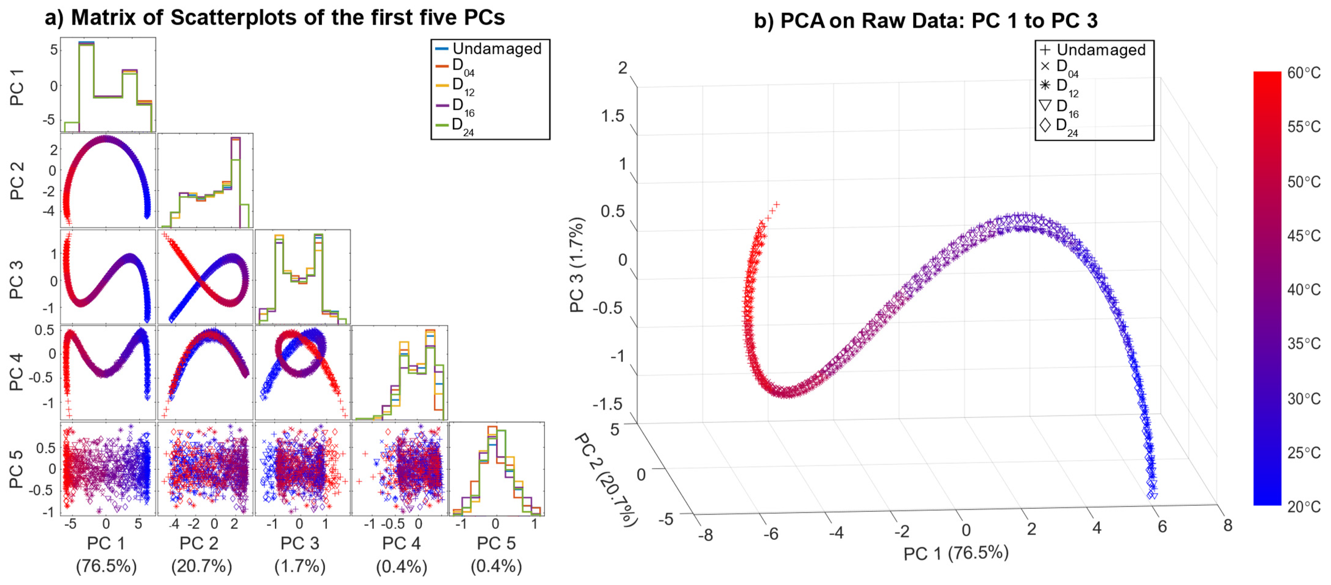
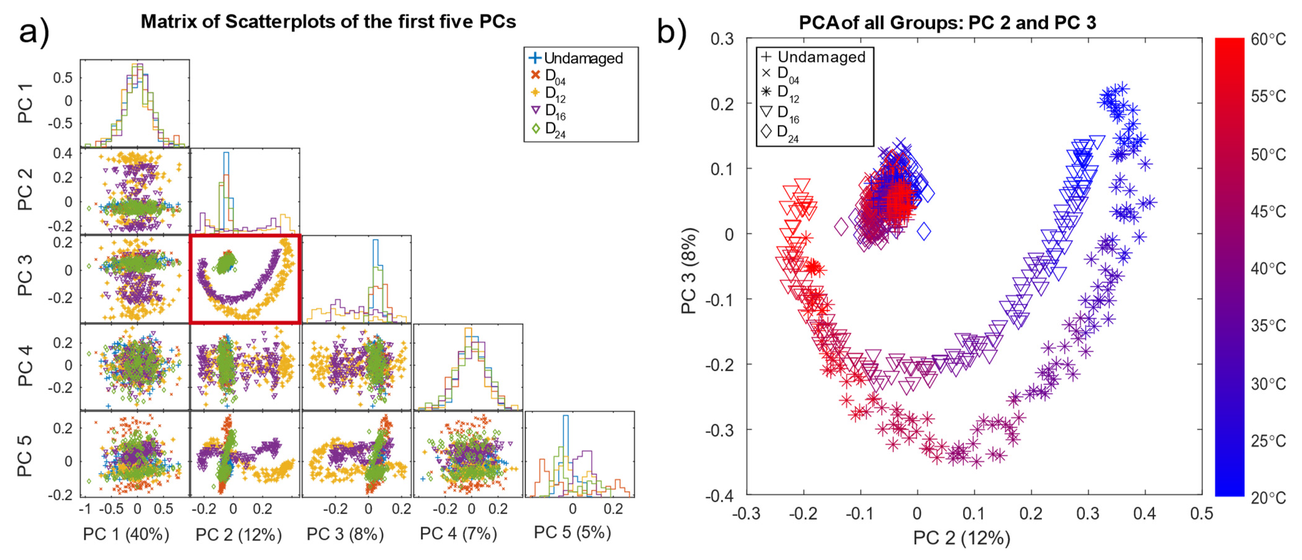
Figure 5a shows the result of the scatterplots of the first five principal components (PC) based on the pre-processed data, with the corresponding variance that each principal component explains and the histograms on the diagonal. Here, the second and third PC (PC2, PC3), indicated by a red box, showed better separability than the remaining PCs. Note that PCA is used here for visualisation of the pre-processed data (OBS + BSS) only, without any additional data treatment.
The scatter plot of PC 2 and PC 3 (
Figure 5b) reveals good separability for damage locations D
12 and D
16 located in the direct signal path between T4 and T9, where waves reflected from and transmitted through the damage (resulting in decreased amplitudes) had a higher impact on the measurements. Since D
04 and D
24 were not in the direct signal path, their influence on the received signal was smaller. D
04, D
24, and the undamaged data formed a cluster in the centre. In addition,
Figure 5b shows all pre-processed measurements coloured by the corresponding temperature. Thus, the crescent-moon shape of the signals for D
12 and D
16 was mainly due to the temperature effect, which was not fully compensated by the OBS + BSS pre-processing.
Figure 5b implies that measurements of D
12 and D
16 at higher temperatures were more difficult to discriminate, as they lay closer to each other as well as to the cluster of the undamaged plate and damages D
04 and D
24.
These plots also show that pre-processing can, at least to a certain degree, suppress temperature effects and highlight damage symptoms. However, the damage cases D04 and D24 overlapped with the undamaged data UG1 and UG2 in the first five PCs, which explains 72% of the variance.
3.2. Results of the Automated Toolbox and Improvement of the Algorithms
In the following, we describe our approach to find a robust model with a high classification rate. When using the standard classifier of the toolbox, the highest resulting test accuracy was 88%, achieved using BFC as a feature extractor and RFE-SVM for feature selection (
Table 4). This classification rate is inadequate, especially for safety-relevant applications.
Table 4 provides further information on how the different FE/FS combinations performed. Here, a user of the toolbox could see that, besides the expected BFC extractor, the SM extractor might be interesting for further analysis, whereas, e.g., ALA is not suitable for FE here.
To increase the performance, the feature extraction method was improved, and the feature selection and classification methods were replaced. Due to the relatively high robustness against incomplete and noisy data in real-life applications, RELIEFF was chosen as the feature selection algorithm [
25,
26]. As a classifier, SVM with RBF kernel was chosen due to its good performance in a comparison of 14 families of classification algorithms on 115 binary datasets [
19].
The BFC extractor of the toolbox initially extracted 5% (1310 features) of the frequency spectrum by ranking them according to the highest amplitude, and extracted those frequencies and their corresponding phase angles. This value was increased up to 10% (2620 features) to also consider features with a lower signal amplitude in the training. To achieve a reasonable computing time, the resulting 2620 features were first reduced to 500 by selecting the features with the highest Pearson correlation to the damage. The final FS method, RELIEFF, reduced the number of features down to 20. This number of features was determined by averaging the obtained feature numbers of the six models in the grid search. This improvement of the toolbox resulted in a damage classification rate of 96.2% (
Table 5) compared to 88%, i.e., reducing the number of misclassified measurements from 118 to 33. A detailed description of the improved algorithms and the procedure is given in
Appendix B.
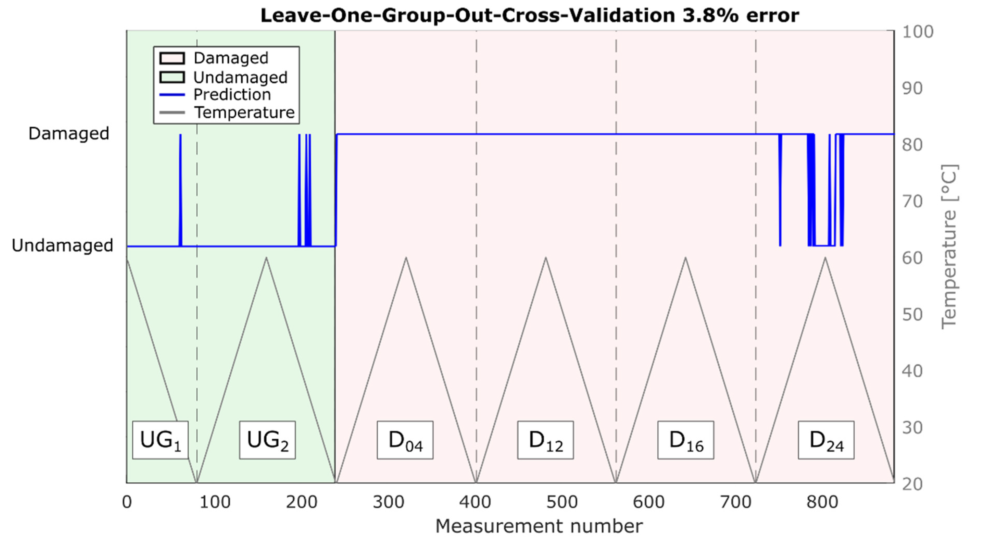
It is worth mentioning that due to the validation strategy (LOGOCV), these results are robust for temperature variations as well as damages at unknown positions. The corresponding predictions are shown in
Figure 6. Note that most misclassifications occurred for measurements of damage at position D
24, which is the location farthest from the direct path in this study (186 mm;
Table 1), in combination with high temperatures (>45 °C).
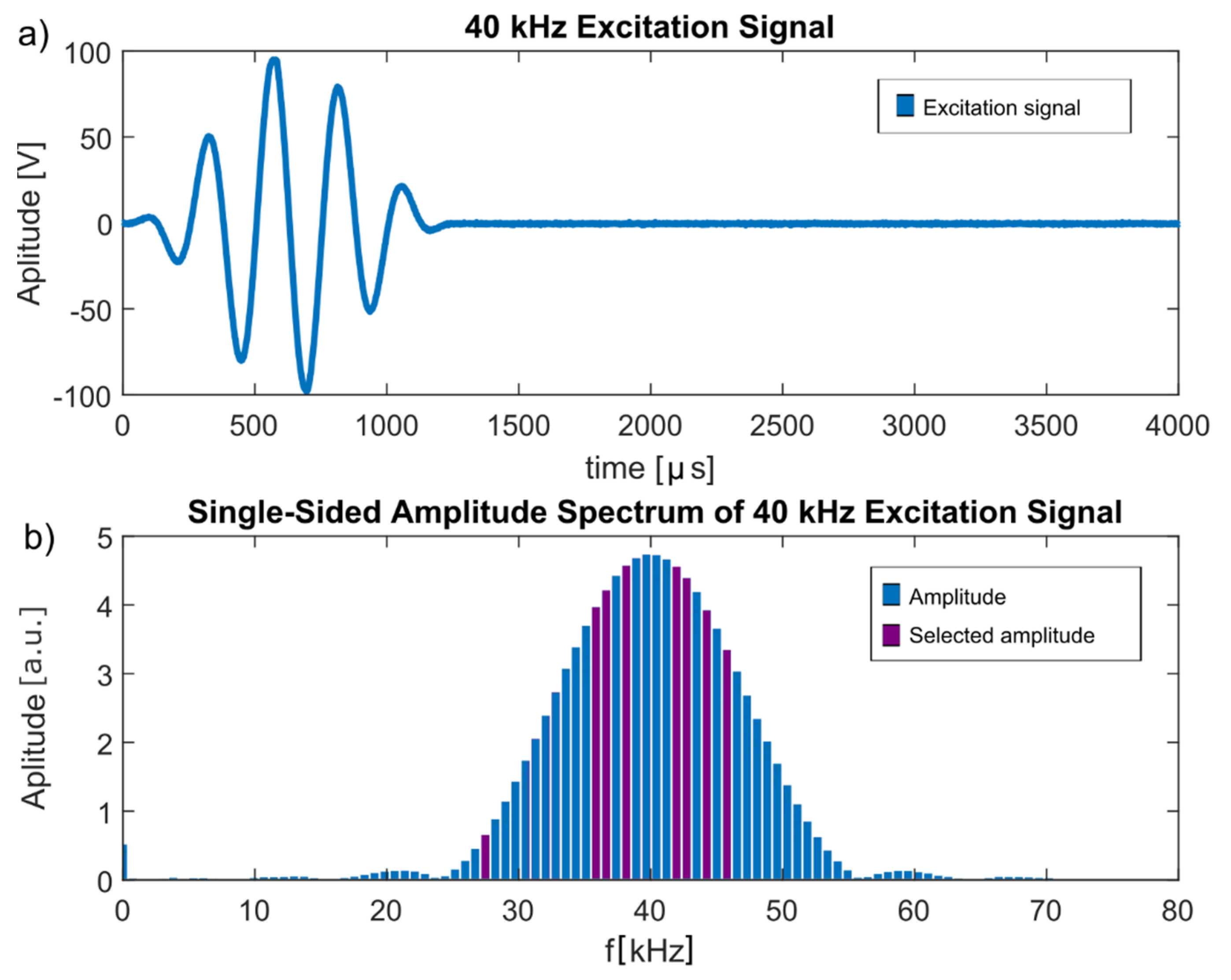
With the proposed transparent FE/FS approach, the ranking of the features that are most often selected for damage detection can help with a physical interpretation. The five highest ranks (eight features) are listed in
Table 6.
These frequencies were all included in the frequency spectrum of the Hann-windowed excitation frequency, as shown in
Figure 7, indicating that they were not a misinterpretation of environmental influences but indeed originated from the excitation signal.
3.3. Influence of the Distance between Damage Location and Signal Path
Incorrectly classified data samples resulted mostly from signals of damage location D
24, which required a considerable extrapolation since this damage location was furthest from the signal path (186 mm;
Table 1), which is believed to have had a significant influence on the ML performance, especially at higher temperatures. Therefore, we performed an additional investigation of the combination of transducers 1 and 7 (
Table 7), where D
24 lay in the direct signal path.
Table 8 shows the distances of each damage location from the direct signal path for this transducer combination.
The results given in
Table 9 show the same tendency as for the combination of transducers 4 and 9: D
24 and D
16 were close to the signal path; thus, they were classified correctly, whereas the accuracy dropped with increasing distance between damage location and signal path. The reduced accuracies for the undamaged cases (UG
1, UG
2) were possibly due to features present in the damage cases being similar to features of the undamaged case; however, this needs to be investigated further.
3.4. Robustness against Temperature Influences
The temperature range tested by Moll et al. [
12] simulates conditions from room temperature up to 60 °C in 0.5 °C steps, making it suitable primarily for indoor applications, e.g., lightweight manipulators for robots [
37]. To also cover outdoor applications, e.g., rotor blades of wind turbines, which have to withstand temperatures in the range from −50 °C to +100 °C [
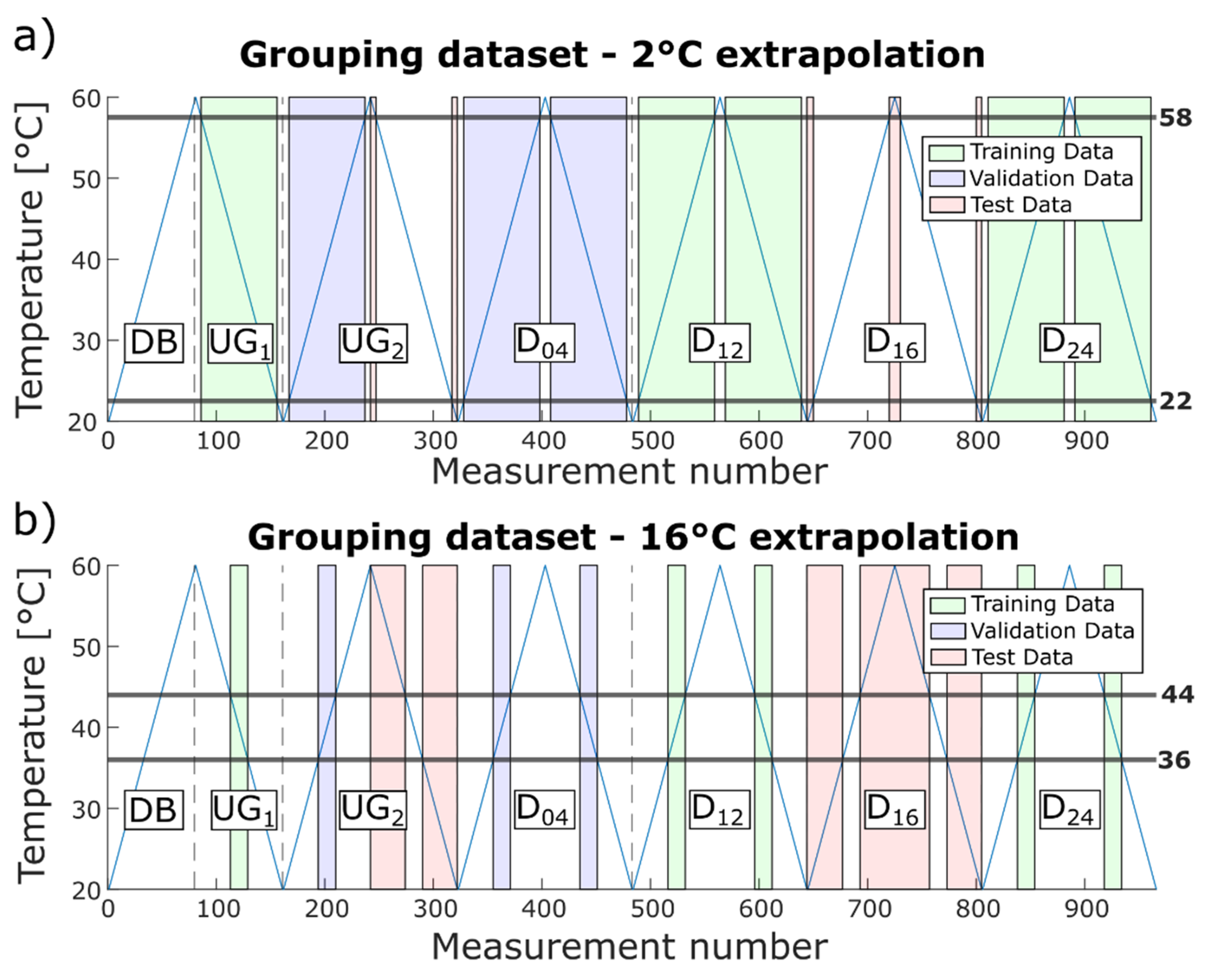
38], the temperature range needs to be extended in future experiments. To investigate the influence of a smaller temperature range while training the ML model, i.e., to check how well the model can extrapolate, a training temperature range was successively reduced, extending the required extrapolation from 2 °C to 16 °C in 2 °C steps. In the scope of this manuscript, extrapolation denotes testing of measurements that were performed outside the trained temperature range. Thus, a model was first built using the temperature range 22.5 °C to 57.5 °C for training and validation, then it was tested for the temperature ranges 20 °C to 22 °C and 58 °C to 60 °C, and then further the training range was further reduced and the test temperature range increased. Within each case, data from UG
1, D
12, and D
24 were used for training, and data from D
04 and the rising temperature flank of UG
2 for validation. The extended temperature range of these data plus the respective data from D
16 and the descending flank of UG
2 were used for testing, as shown in
Figure 8a,b for 2 °C and 16 °C extrapolation, respectively.
Note that further extrapolation is not meaningful since the size of the training data set was reduced with every step, decreasing the statistical significance. For 16 °C extrapolation, the training data (green areas in
Figure 8b) only contained 75 measurements in the range of 36.5 °C to 43.5 °C.
Table 10 shows the test accuracies achieved for each temperature extrapolation step. The ML model extrapolated up to 6 °C without loss of performance and had only a slight decrease in performance for temperature extrapolations up to 10 °C, indicating that the model is fairly robust to temperature influences. This might allow a model to be built based on data from a lab environment that could still achieve acceptable performance under real operating conditions. Note that extrapolation over 12 °C corresponds to a training range from 32.5 °C to 47.5 °C, i.e., ΔT = 15 °C. Thus, only approx. one third of the overall temperature range is necessary to achieve an accuracy of 93.6% even for previously unknown damage locations.
3.5. Comparison to a State-of-the-Art Neural Network
Since neural networks (NN) are nowadays often used for SHM applications [
39,
40,
41], we benchmarked our approach against a neural network approach reported for the same dataset [
9]. In this study, Mariani et al. first tested several deep learning algorithms, namely, a multilayer perceptron, a recurrent neural network with long short-term memory, and a WaveNet-based causal dilated convolutional neural network (CNN), on a reference guided wave SHM dataset using a threshold-based OBS + BSS as the benchmark. They found that multilayer perceptrons and recurrent neural networks were not able to significantly outperform OBS + BSS, whereas the causal dilated CNN delivered high accuracy within reasonable training time and was therefore applied to the experimental guided wave dataset for varying temperature [
12]. Mariani et al. achieved 100% accuracy on the testing data for the transducer combination T
4 to T
10 with a high-pass filter (Butterworth), down sampling (factor 6), and BSS (undamaged plate at 40 °C) as pre-processing. A more detailed description as well as the architecture of the causal dilated CNN can be found in the original paper [
9].
To compare our approach with these results for the causal dilated CNN, we also evaluated the transducer combination T4 and T10 for model building and replicated the grouping of Mariani et al. for training, validation, and testing data. Thus, training data contained D16, D24, and 50% of UG2; validation data contained D12 and 25% of UG2; and testing data contain D04 and 25% of UG2. The split of UG2 into the corresponding groups was based on a training–validation–training–testing pattern with a 1.5 °C step size (e.g., data from 20 °C–21.5 °C were used for training, 22 °C–23.5 °C for validation, 24 °C–25.5 °C for training, 26 °C–27.5 °C for testing, 28 °C–29.5 °C again for training, etc.).
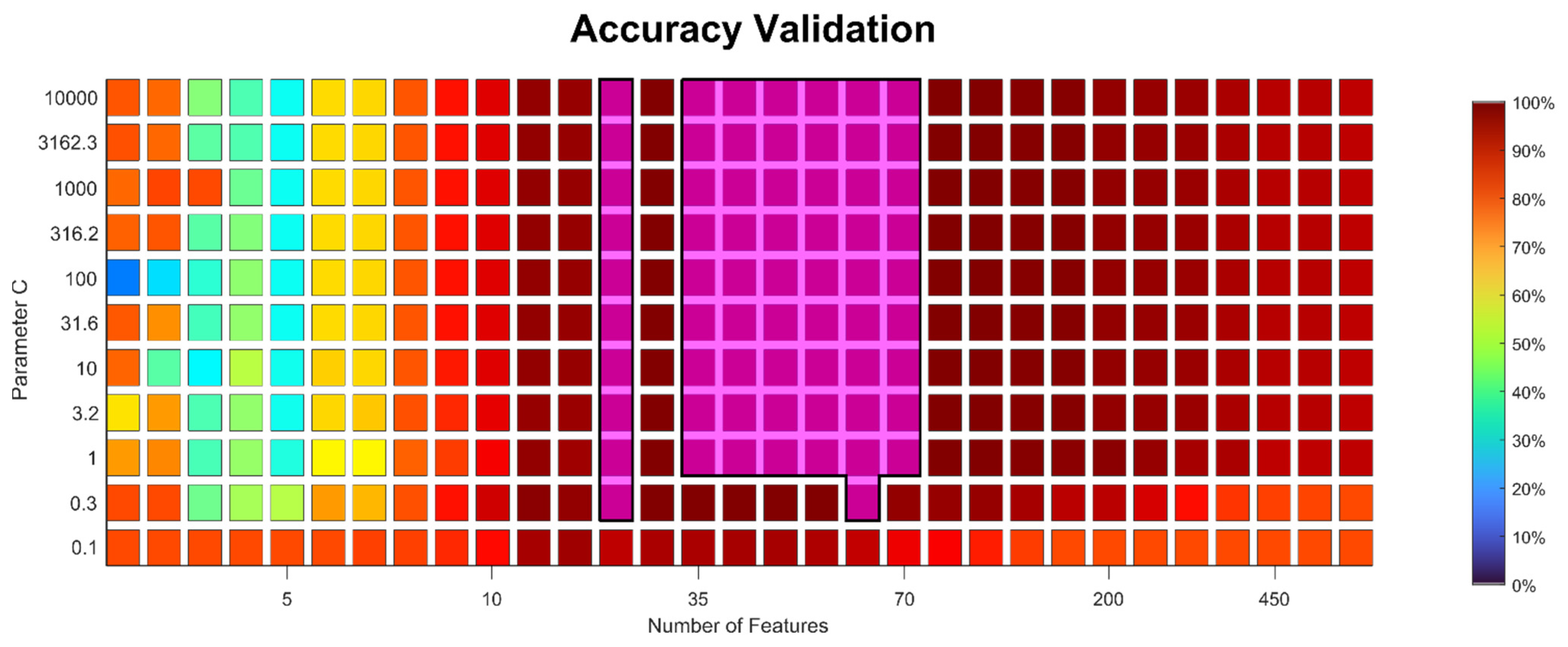
The model was built using the improved approach described above, with BFC as a feature extractor, PCC for feature pre-selection, RELIEFF for the final feature selection, and SVM with RBF kernel as a classifier. Out of the possible combinations for the hyper-parameters, the algorithm selected 30 as the best number of features and 10,000 as the value for parameter C. Actually, a wide range of hyper-parameter combinations achieved a validation accuracy of 100%, showing that the approach is robust (
Appendix C,
Figure A2). After hyper-parameter selection and before applying the model on the test data, it was again trained with all training and validation data. The achieved prediction accuracy of 100% for damage D
04 matches the result reported by Mariani et al.
The computational time for our model was 185 s on an Intel® Core™ i7 8650U CPU, which is also similar to the 5 min training time for the causal dilated CNN reported by Mariani et al. using one NVIDIA® Quadro RTX™ 6000 GPU (2000 epochs). Note, however, that the CPU used in our study only has a theoretical computational performance of 0.442 TFLOPS (tera floating-point operations per second) compared to 16.3 TFLOPS of the GPU.
At first glance it might seem that the causal dilated CNN required less data pre-processing. However, hyper-parameter optimisation (HPO) is not described by Mariani et al. in their study. It is well known that HPO of NN models often requires significant (hardware and human) resources. Over the last few years, different approaches [
42,
43,
44] have been proposed to solve this problem. Existing methods and frameworks to find a proper architecture and HPO of NNs are often computationally expensive and/or application-specific [
43,
44]. On the other hand, HPO for our proposed approach is simple and clear, as demonstrated by
Figure A2 (
Appendix C), which is one of the advantages of using classical ML methods (feature extraction/feature selection/simple classification) instead of deep NN models. Furthermore, our approach directly provides relevant features, i.e., a physically interpretable result, whereas NN models are often a black box and require significant additional effort to allow for interpretation.


 ,
, 


