
An Experimental Urban Case Study with Various Data Sources and a Model for Traffic Estimation


Abstract
:1. Introduction
2. Related Works
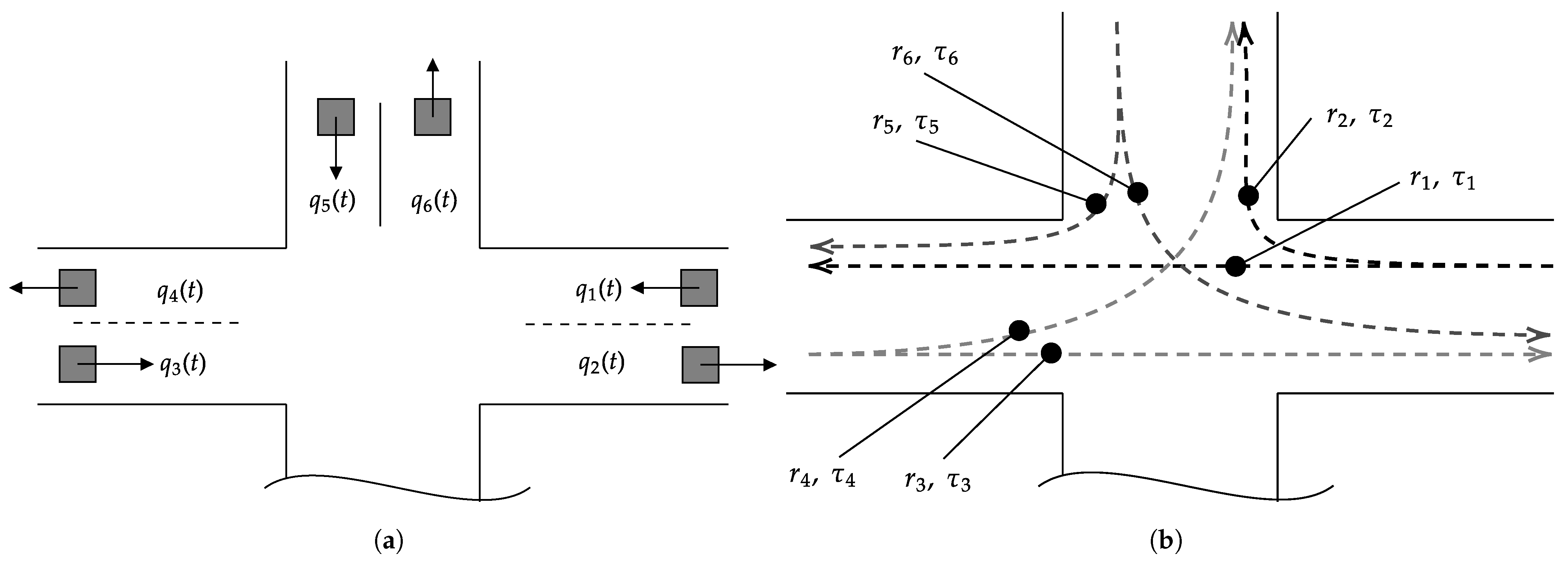
3. Methodology for Representing Urban Traffic States
4. Travel Time Estimation Methodology
4.1. Feature Engineering
- : 5% random data sample from e.g., CAVs;
- : Average headway (s) when a traffic light is green;
- : Progressed flow at an intersection (veh/h);
- : Average occupancy of LDs (%);
- : Average red/green phase count (-).
4.2. Mlr Model Definition
4.3. Baseline Model Specification
4.4. Final Model Specification
4.5. Performance Metrics
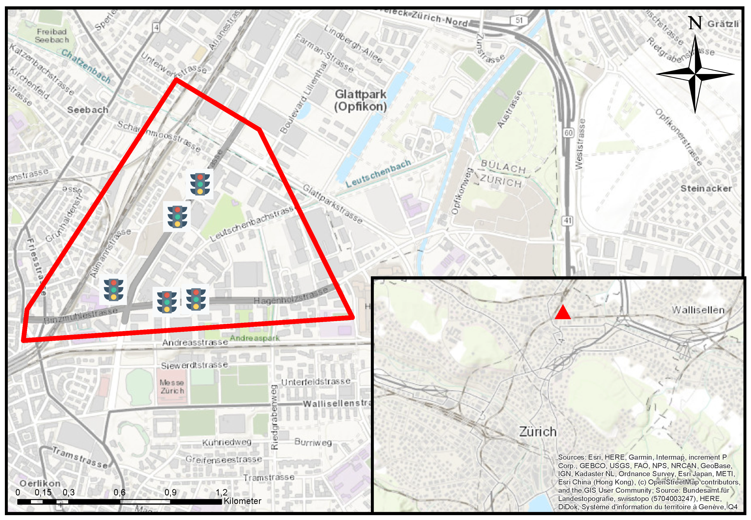
5. Description of Experimental Campaign and Data Sources
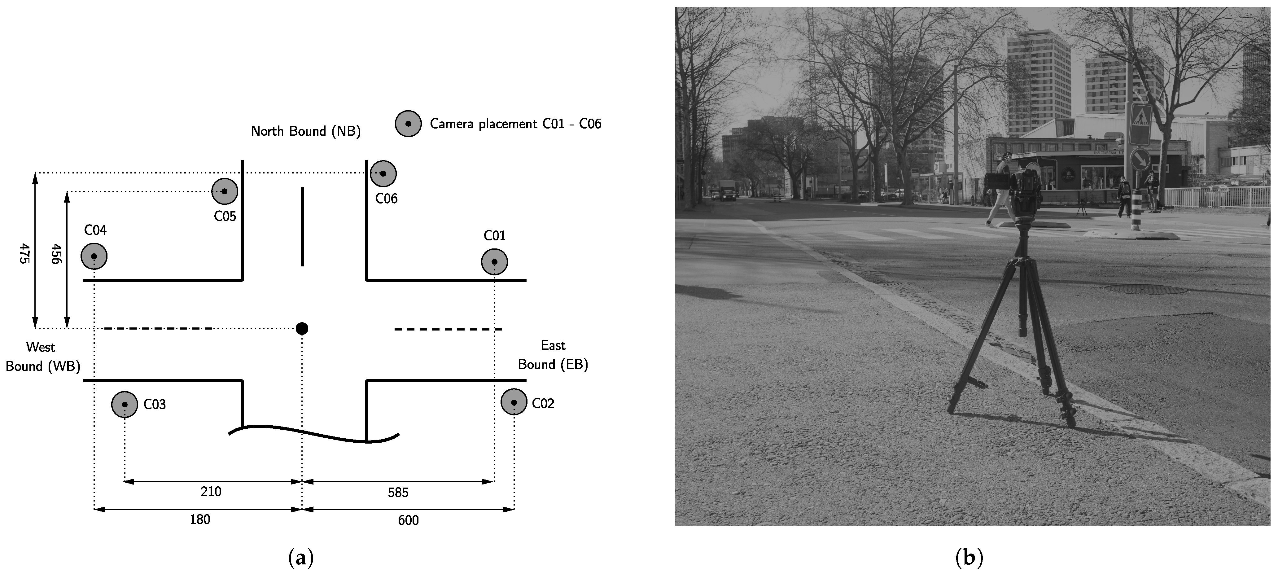
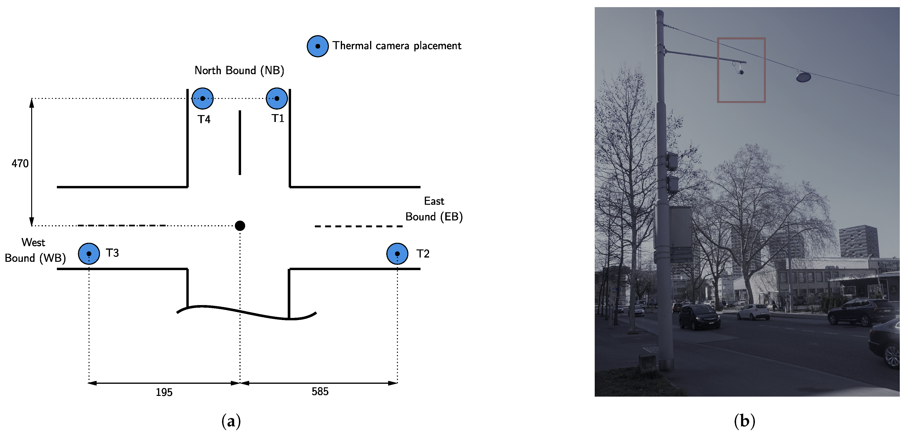
5.1. Experimental Campaign with Video Cameras
5.2. Data Sources for Sensor Assessment
6. Results
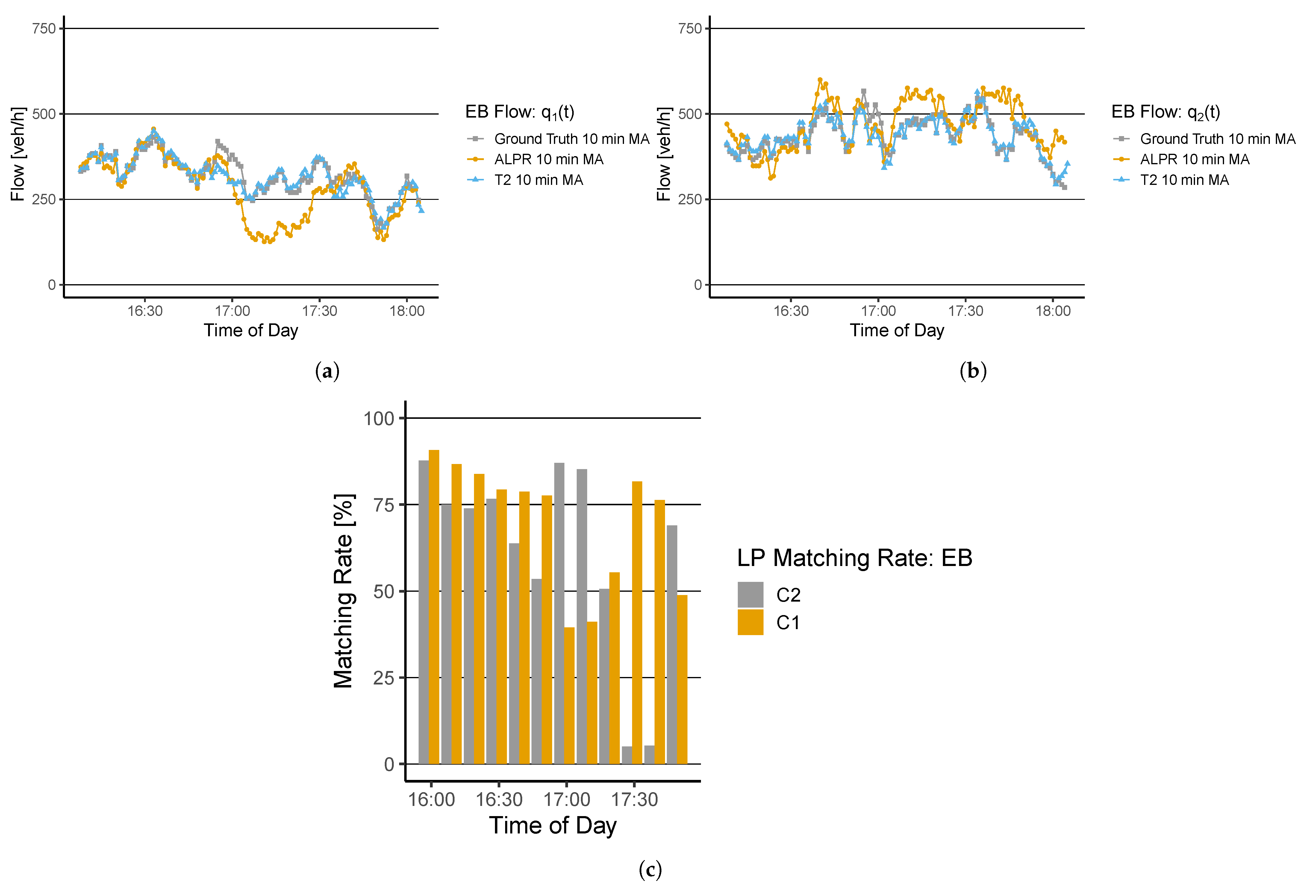
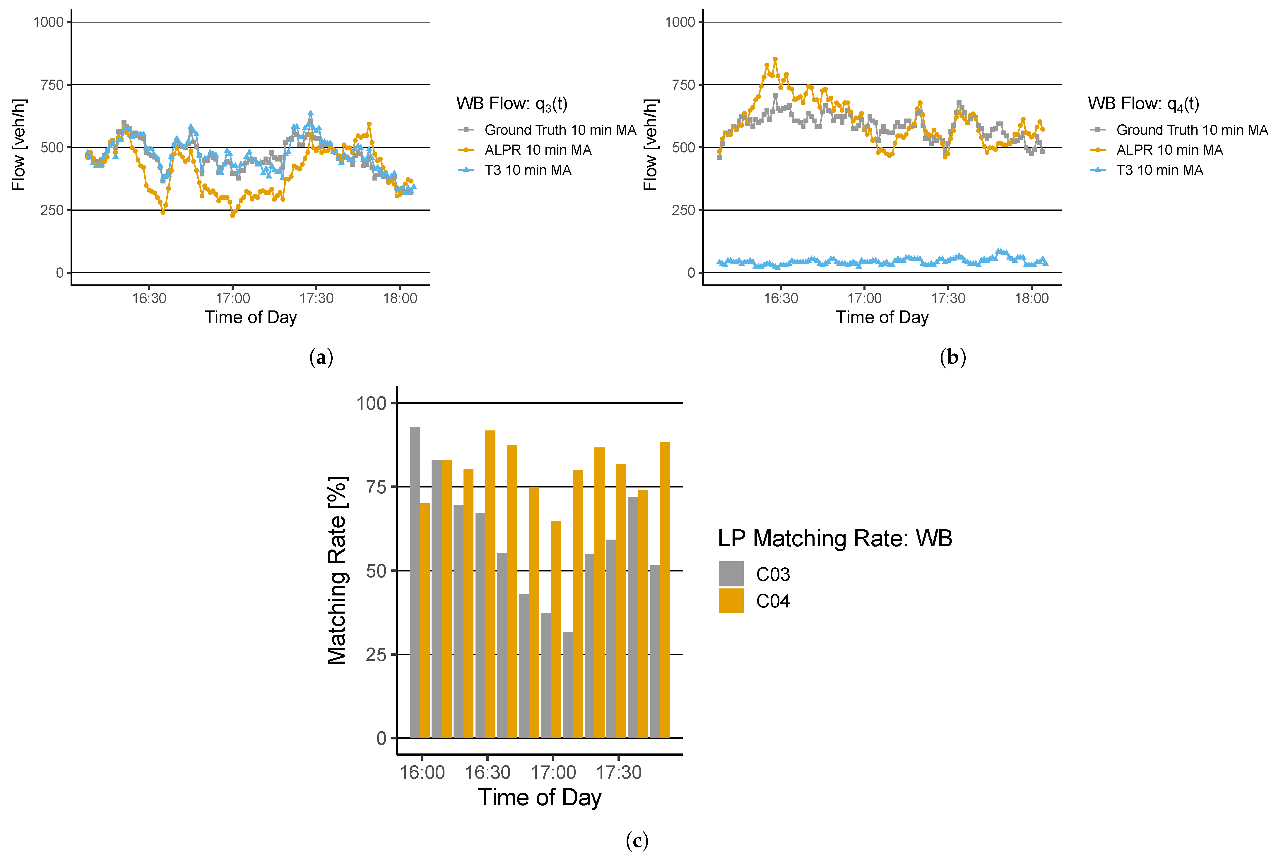
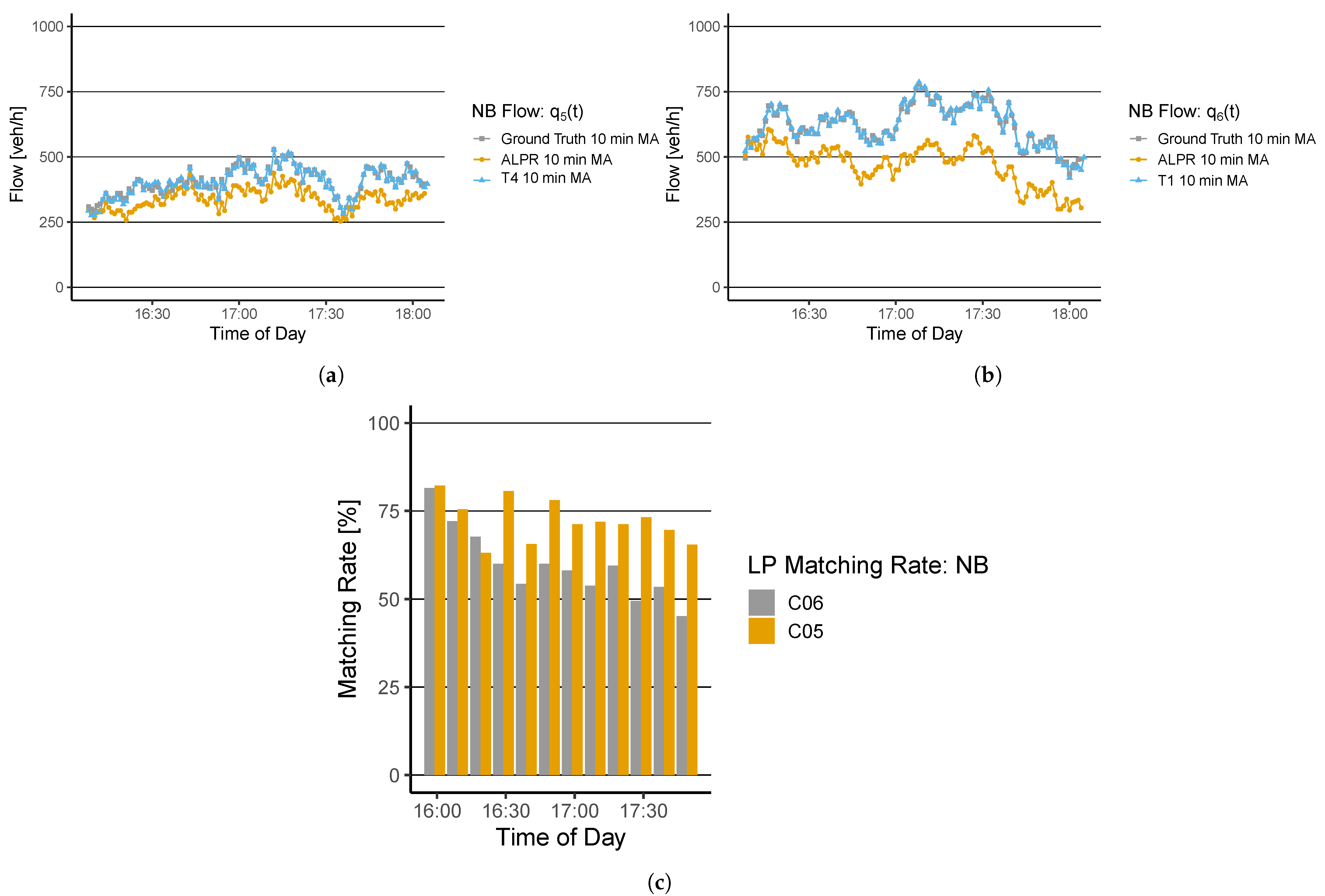
6.1. Traffic State Representation and Sensor-Based Assessment
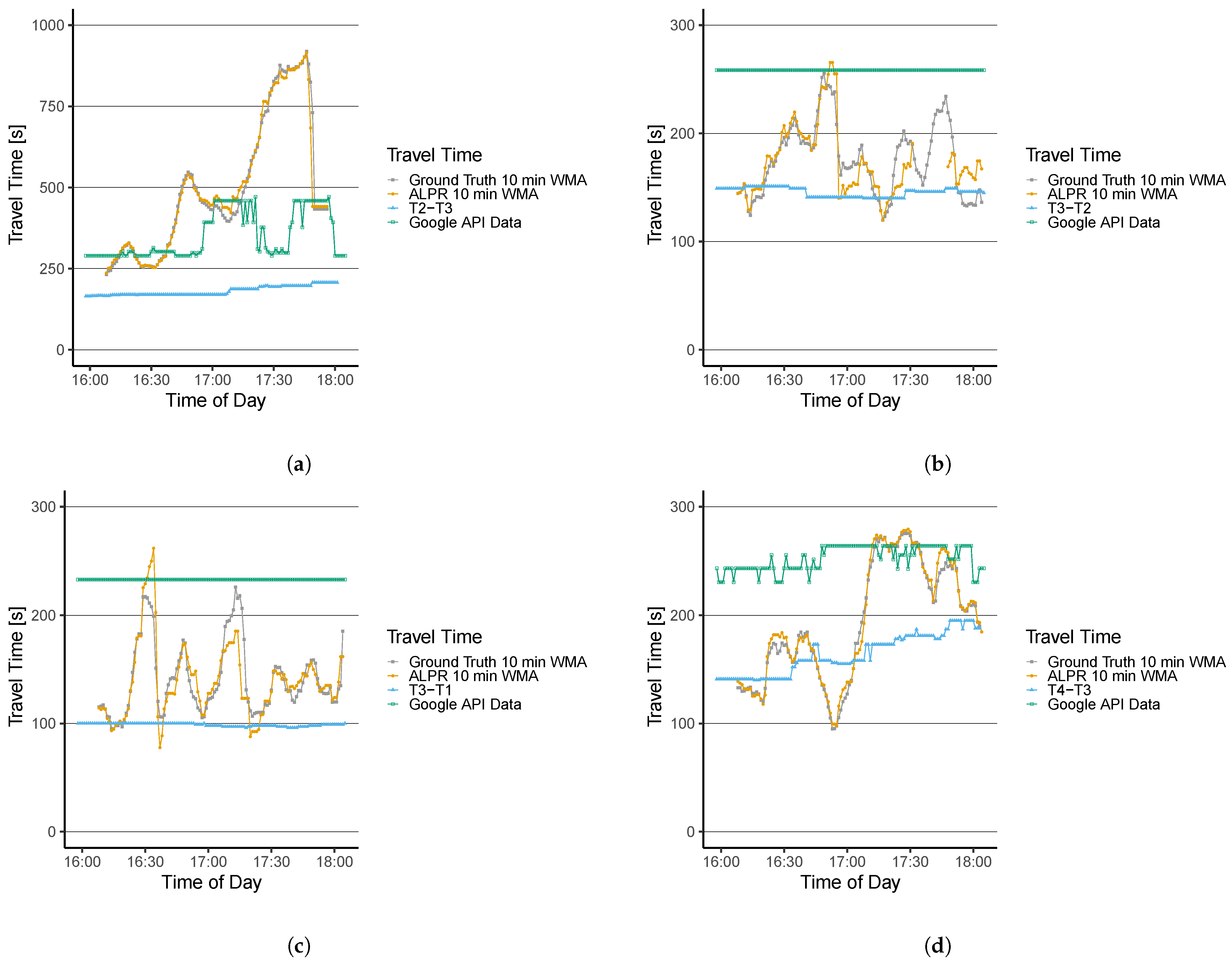
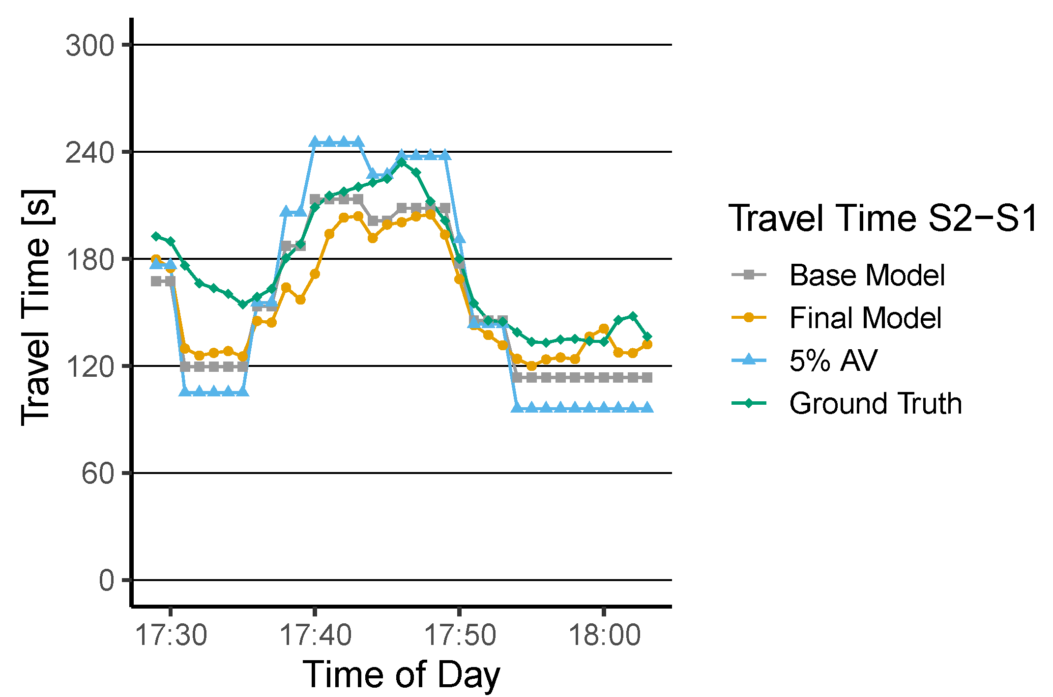
6.2. Travel Time Estimation Assessment
7. Discussion
7.1. Traffic States–Traffic Flow
7.2. Traffic States–Travel Times
7.3. Travel Time Estimation Models
8. Conclusions
Author Contributions
Funding
Institutional Review Board Statement
Informed Consent Statement
Data Availability Statement
Conflicts of Interest
References
- Kouvelas, A.; Chow, A.; Gonzales, E.; Yildirimoglu, M.; Carlson, R.C. Emerging Information and Communication Technologies for Traffic Estimation and Control. J. Adv. Transp. 2018, 2018, 8498054. [Google Scholar] [CrossRef]
- Bachmann, C.; Roorda, M.J.; Abdulhai, B.; Moshiri, B. Fusing a Bluetooth Traffic Monitoring System With Loop Detector Data for Improved Freeway Traffic Speed Estimation. J. Intell. Transp. Syst. 2013, 17, 152–164. [Google Scholar] [CrossRef]
- Zheng, F. Modelling Urban Travel Times. Ph.D. Thesis, TRAIL Research School, Delft, The Netherlands, 12 July 2011. [Google Scholar]
- Genser, A.; Kouvelas, A. Optimum route guidance in multi-region networks. A linear approach. In Proceedings of the 99th Annual Meeting of the Transportation Research Board, Washington, DC, USA, 12–16 January 2020. [Google Scholar] [CrossRef]
- Genser, A.; Kouvelas, A. Dynamic optimal congestion pricing in multi-region urban networks by application of a Multi-Layer-Neural network. Transp. Res. Part C Emerg. Technol. 2022, 134, 103485. [Google Scholar] [CrossRef]
- Genser, A.; Ambühl, L.; Yang, K.; Menendez, M.; Kouvelas, A. Time-to-Green predictions: A framework to enhance SPaT messages using machine learning. In Proceedings of the 2020 IEEE 23rd International Conference on Intelligent Transportation Systems (ITSC), Rhodes, Greece, 20–23 September 2020; pp. 1–6. [Google Scholar]
- Chavoshi, K.; Genser, A.; Kouvelas, A. A Pairing Algorithm for Conflict-Free Crossings of Automated Vehicles at Lightless Intersections. Electronics 2021, 10, 1702. [Google Scholar] [CrossRef]
- Yildirimoglu, M.; Geroliminis, N. Experienced travel time prediction for congested freeways. Transp. Res. Part B Methodol. 2013, 53, 45–63. [Google Scholar] [CrossRef] [Green Version]
- Haghani, A.; Hamedi, M.; Sadabadi, K.F.; Young, S.; Tarnoff, P. Data Collection of Freeway Travel Time Ground Truth with Bluetooth Sensors. Transp. Res. Rec. 2010, 2160, 60–68. [Google Scholar] [CrossRef]
- Sharifi, E.; Hamedi, M.; Haghani, A.; Sadrsadat, H. Analysis of Vehicle Detection Rate for Bluetooth Traffic Sensors: A Case Study in Maryland and Delaware. In Proceedings of the 18th ITS World Congress, Orlando, FL, USA, 16–20 October 2011. [Google Scholar]
- Erkan, I.; Hastemoglu, H. Bluetooth as a traffic sensor for stream travel time estimation under Bogazici Bosporus conditions in Turkey. J. Mod. Transp. 2016, 24, 207–214. [Google Scholar] [CrossRef] [Green Version]
- Barcelö, J.; Montero, L.; Marqués, L.; Carmona, C. Travel Time Forecasting and Dynamic Origin-Destination Estimation for Freeways Based on Bluetooth Traffic Monitoring. Transp. Res. Rec. 2010, 2175, 19–27. [Google Scholar] [CrossRef] [Green Version]
- Barceló, J.; Montero, L.; Bullejos, M.; Serch, O.; Carmona, C. A Kalman Filter Approach for the Estimation of Time Dependent OD Matrices Exploiting Bluetooth Traffic Data Collection. In Proceedings of the 91st Transportation Research Board 2012 Annual Meeting, Washington, DC, USA, 22–26 January 2012; pp. 1–16. [Google Scholar]
- Elliott, T.; Lumley, T. Modelling the travel time of transit vehicles in real-time through a GTFS-based road network using GPS vehicle locations. Aust. N. Z. J. Stat. 2020, 62, 153–167. [Google Scholar] [CrossRef]
- Abedi, N.; Bhaskar, A.; Chung, E.; Miska, M. Assessment of antenna characteristic effects on pedestrian and cyclists travel-time estimation based on Bluetooth and WiFi MAC addresses. Transp. Res. Part C Emerg. Technol. 2015, 60, 124–141. [Google Scholar] [CrossRef]
- Shen, L. Practical approach for travel time estimation from point traffic detector data. J. Adv. Transp. 2013, 47, 526–535. [Google Scholar] [CrossRef]
- Yeon, J.; Elefteriadou, L.; Lawphongpanich, S. Travel time estimation on a freeway using Discrete Time Markov Chains. Transp. Res. Part B Methodol. 2008, 42, 325–338. [Google Scholar] [CrossRef]
- Bhaskar, A.; Chung, E.; Dumont, A.G. Fusing Loop Detector and Probe Vehicle Data to Estimate Travel Time Statistics on Signalized Urban Networks. Comput.-Aided Civ. Infrastruct. Eng. 2011, 26, 433–450. [Google Scholar] [CrossRef] [Green Version]
- Bock, J.; Krajewski, R.; Moers, T.; Runde, S.; Vater, L.; Eckstein, L. The inD Dataset: A Drone Dataset of Naturalistic Road User Trajectories at German Intersections. In Proceedings of the 2020 IEEE Intelligent Vehicles Symposium (IV), Las Vegas, NV, USA, 19 October–13 November 2020; pp. 1929–1934. [Google Scholar]
- Lyman, K.; Bertini, R.L. Using Travel Time Reliability Measures to Improve Regional Transportation Planning and Operations. Transp. Res. Rec. 2008, 2046, 1–10. [Google Scholar] [CrossRef] [Green Version]
- Chen, Z.; Fan, W. Data analytics approach for travel time reliability pattern analysis and prediction. J. Mod. Transp. 2019, 27, 250–265. [Google Scholar] [CrossRef] [Green Version]
- Benesty, J.; Chen, J.; Huang, Y.; Cohen, I. Noise Reduction in Speech Processing; Springer: Berlin/Heidelberg, Germany, 2009. [Google Scholar]
- Kim, S.; Kim, H. A new metric of absolute percentage error for intermittent demand forecasts. Int. J. Forecast. 2016, 32, 669–679. [Google Scholar] [CrossRef]
- Branston, D.; van Zuylen, H. The estimation of saturation flow, effective green time and passenger car equivalents at traffic signals by multiple linear regression. Transp. Res. 1978, 12, 47–53. [Google Scholar] [CrossRef]
- TomTom International, BV. Zurich Traffic Report. Available online: https://www.tomtom.com/en_gb/traffic-index/zurich-traffic (accessed on 4 July 2021).
- Silva, S.M.; Jung, C.R. License plate detection and recognition in unconstrained scenarios. In Proceedings of the 2018 European Conference on Computer Vision (ECCV), Munich, Germany, 8–14 September 2018; pp. 580–596. [Google Scholar]
- Gade, R.; Moeslund, T.B. Thermal cameras and applications: A survey. Mach. Vis. Appl. 2014, 25, 245–262. [Google Scholar] [CrossRef] [Green Version]
- Fu, T.; Stipancic, J.; Zangenehpour, S.; Miranda-Moreno, L.; Saunier, N. Automatic traffic data collection under varying lighting and temperature conditions in multimodal environments: Thermal versus visible spectrum video-based systems. J. Adv. Transp. 2017, 2017, 5142732. [Google Scholar] [CrossRef]
- Ding, F.; Chen, X.; He, S.; Shou, G.; Zhang, Z.; Zhou, Y. Evaluation of a wi-fi signal based system for freeway traffic states monitoring: An exploratory field test. Sensors 2019, 19, 409. [Google Scholar] [CrossRef] [PubMed] [Green Version]
- Kwong, K.; Kavaler, R.; Rajagopal, R.; Varaiya, P. Arterial travel time estimation based on vehicle re-identification using wireless magnetic sensors. Transp. Res. Part C Emerg. Technol. 2009, 17, 586–606. [Google Scholar] [CrossRef]
- Bakhtan, M.A.H.; Abdullah, M.; Rahman, A.A. A review on License Plate Recognition system algorithms. In Proceedings of the 2016 International Conference on Information and Communication Technology (ICICTM), Kuala Lumpur, Malaysia, 16–17 May 2016; pp. 84–89. [Google Scholar]
- Redmon, J.; Divvala, S.; Girshick, R.; Farhadi, A. You Only Look Once: Unified, Real-Time Object Detection. In Proceedings of the 2016 IEEE Conference on Computer Vision and Pattern Recognition (CVPR), Las Vegas, NV, USA, 27–30 June 2016; pp. 779–788. [Google Scholar]
- Google Developers. Distance Matrix API—Documentation. Available online: https://developers.google.com/maps/documentation/distance-matrix/overview (accessed on 23 July 2021).

| LP | TC | LP | TC | LP | TC | LP | TC | LP | TC | LP | TC | |
| [-] | 0.81 | 0.91 | 0.61 | 0.93 | 0.58 | 0.94 | 0.73 | 0.00 | 0.58 | 0.94 | 0.76 | 0.99 |
| [%] | 15.54 | 4.83 | 12.64 | 3.33 | 17.20 | 3.86 | 9.17 | 92.45 | 17.20 | 3.86 | 24.42 | 1.22 |
| LP | TC | G | LP | TC | G | LP | TC | G | LP | TC | G | |
| [-] | 0.99 | 0.71 | 0.27 | 0.84 | −0.11 | NA | 0.85 | −0.13 | NA | 0.99 | 0.72 | 0.33 |
| [%] | 3.14 | 58.07 | 25.95 | 8.04 | 18.36 | 50.64 | 7.51 | 26.76 | 73.38 | 2.73 | 20.60 | 45.49 |
| [-] | MAPE [%] | |
|---|---|---|
| 5% sample | - | 18.10 |
| Base Model | 0.40 | 11.62 |
| Final Model | 0.81 | 10.92 |
Publisher’s Note: MDPI stays neutral with regard to jurisdictional claims in published maps and institutional affiliations. |
© 2021 by the authors. Licensee MDPI, Basel, Switzerland. This article is an open access article distributed under the terms and conditions of the Creative Commons Attribution (CC BY) license (https://creativecommons.org/licenses/by/4.0/).
Share and Cite
Genser, A.; Hautle, N.; Makridis, M.; Kouvelas, A. An Experimental Urban Case Study with Various Data Sources and a Model for Traffic Estimation. Sensors 2022, 22, 144. https://doi.org/10.3390/s22010144
Genser A, Hautle N, Makridis M, Kouvelas A. An Experimental Urban Case Study with Various Data Sources and a Model for Traffic Estimation. Sensors. 2022; 22(1):144. https://doi.org/10.3390/s22010144
Chicago/Turabian StyleGenser, Alexander, Noel Hautle, Michail Makridis, and Anastasios Kouvelas. 2022. "An Experimental Urban Case Study with Various Data Sources and a Model for Traffic Estimation" Sensors 22, no. 1: 144. https://doi.org/10.3390/s22010144
APA StyleGenser, A., Hautle, N., Makridis, M., & Kouvelas, A. (2022). An Experimental Urban Case Study with Various Data Sources and a Model for Traffic Estimation. Sensors, 22(1), 144. https://doi.org/10.3390/s22010144