
The Dependence of Flue Pipe Airflow Parameters on the Proximity of an Obstacle to the Pipe’s Mouth


Abstract
:1. Introduction
2. Measurements
3. Data Analysis
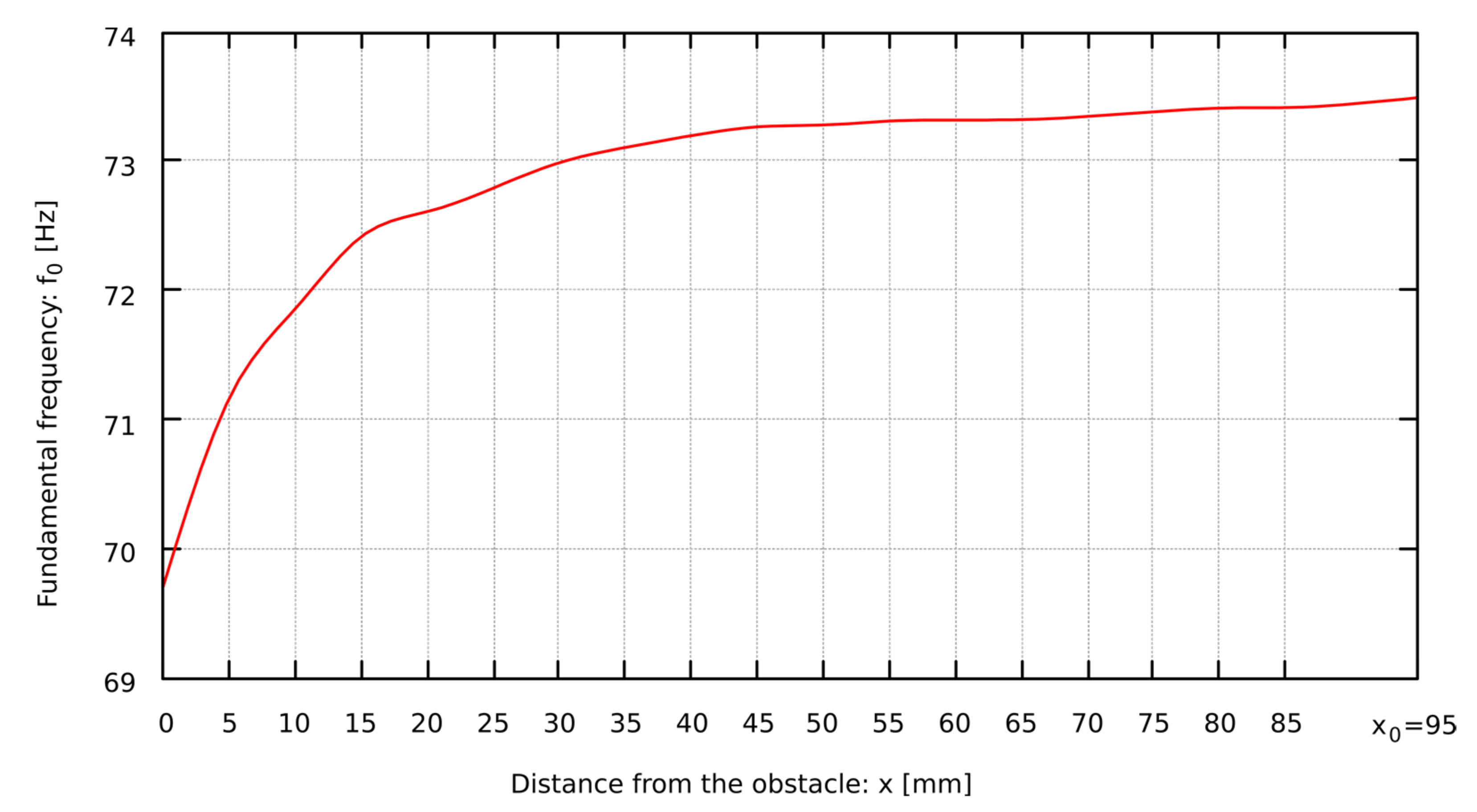
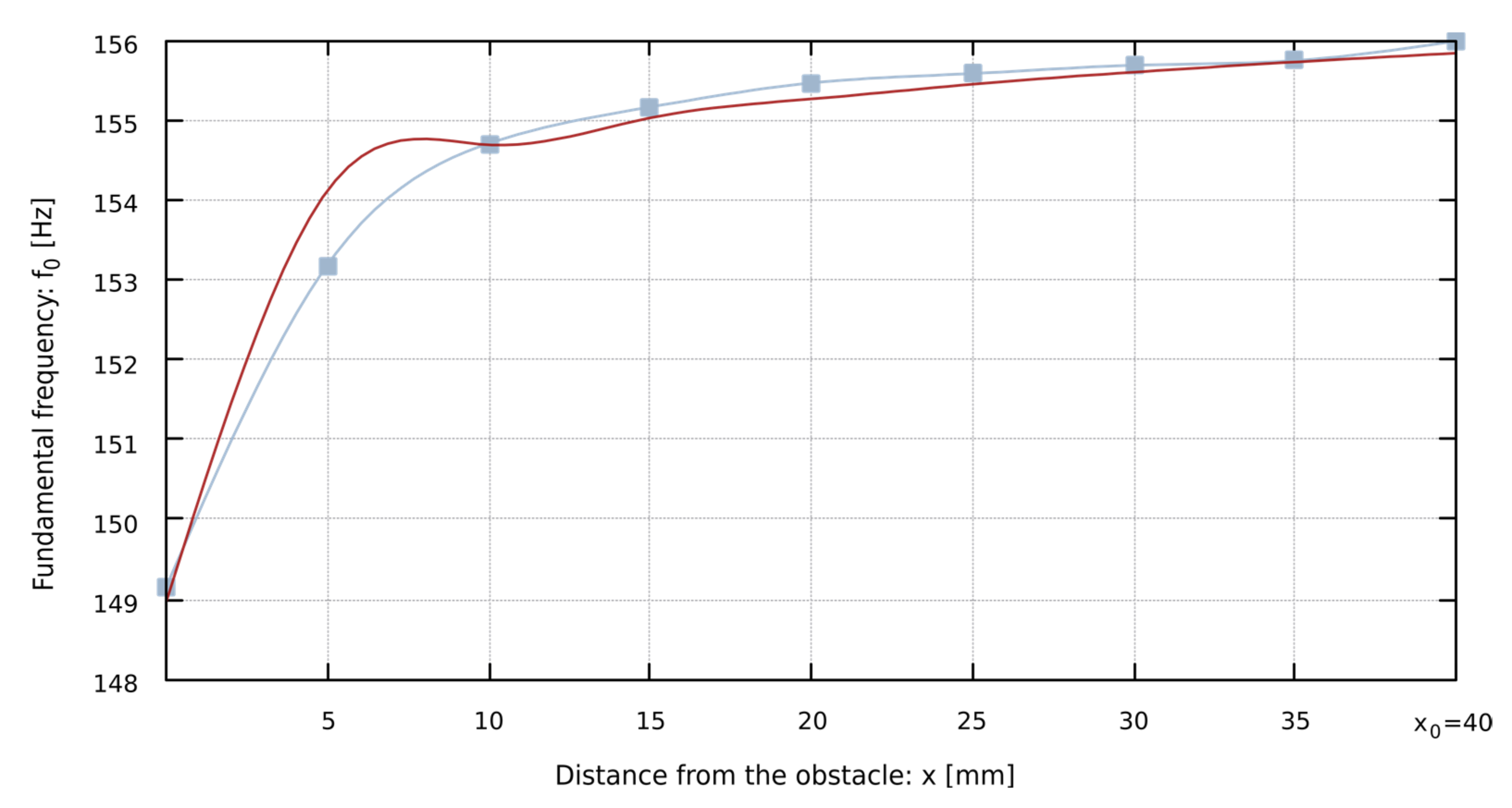
- The fundamental frequency of the pipe decreases as the obstacle is closer to the lip. The changes of the pipe sound frequency depending on the distance of the obstacle to the mouth of the pipe are presented in Table 2;
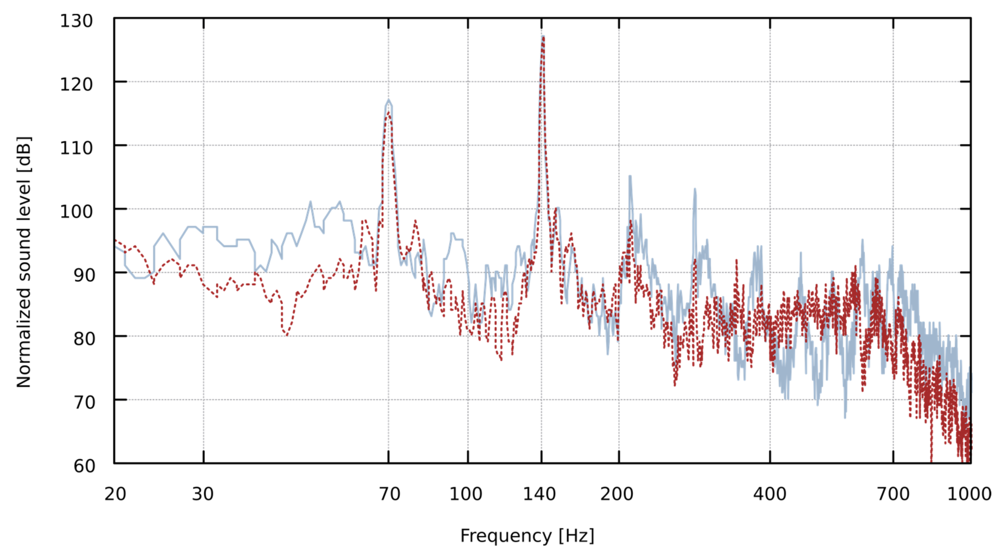
- The spectrum of the sound recorded at the mouth of the pipe may differ significantly from the spectrum of the sound at the top of the resonator (i.a. significant difference in the number of harmonics may be observed);
- The fundamental frequency of the pipe, measured at the top of the pipe resonator, is sometimes different from the fundamental frequency measured at the lip of the pipe. It can be seen in the spectrum, especially on the logarithmic frequency scale, as the harmonics of the sound do not overlap, as shown in Figure 3;
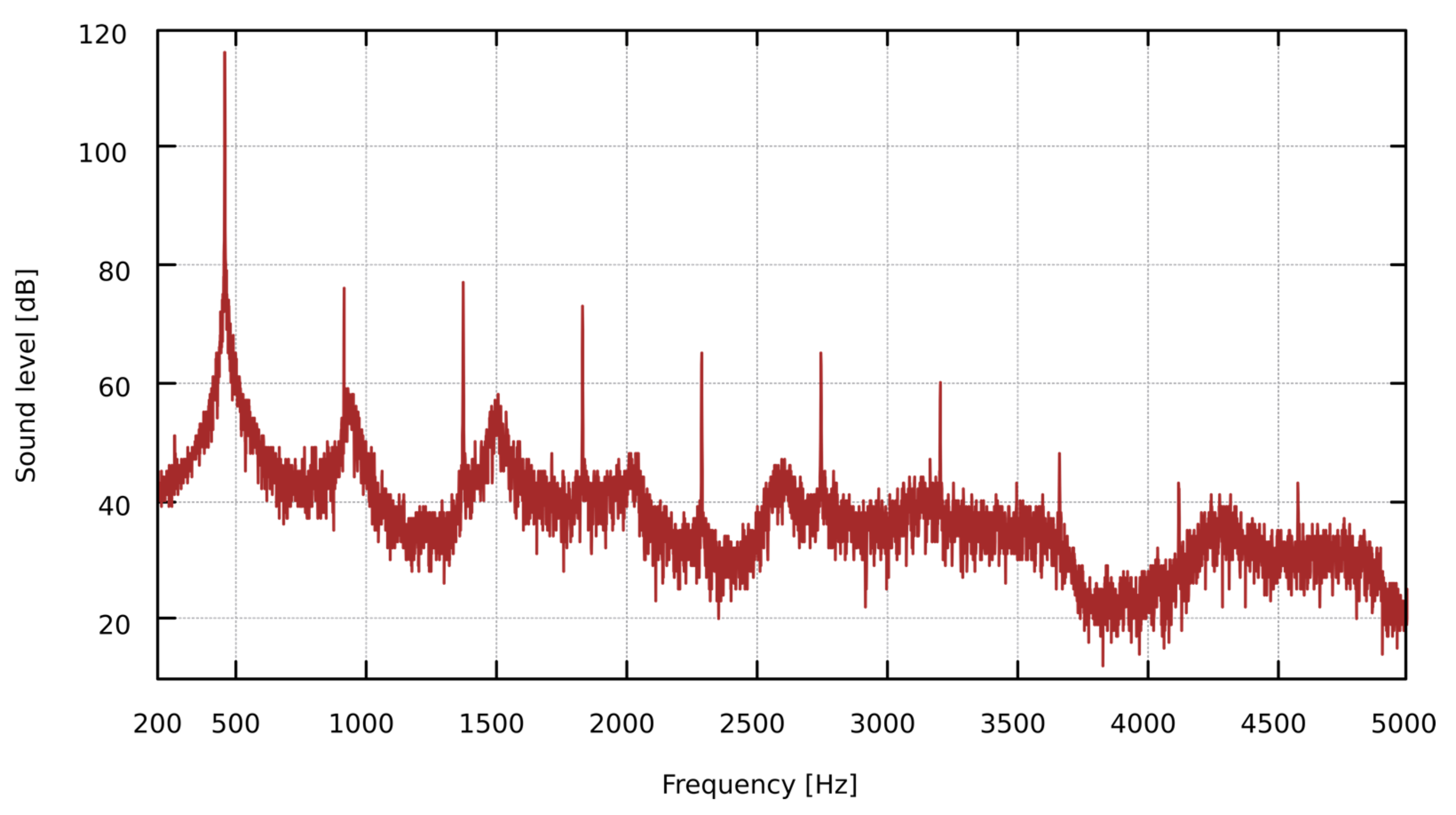
- In the spectrum of some pipes, there are additional components that are not harmonics of the fundamental frequency of the pipe, see Figure 4.
4. Interval Calculus
5. Fundamentals of a Sound Generation in a Labial Pipe
6. Results
6.1. Determination of Strouhal and Reynolds Numbers for Labial Pipes
6.2. The Influence of an Obstacle on the Change of Flow Velocity
6.3. The Dependence of the Fundamental Frequency on the Change in the Distance of the Obstacle from the Pipe’s Mouth
7. Discussion
8. Conclusions
- The fundamental frequency of the sound is directly proportional to the speed of the airflow in the pipe’s mouth;
- The speed of the airflow in the pipe’s mouth increases with the distance of the obstacle from the pipe’s mouth;
- The value of the Reynolds number in the pipe increases with the distance of the obstacle from the pipe’s mouth;
- The value of the Strouhal number for a labial pipe does not change significantly and can be approximated by a constant value.
Author Contributions
Funding
Institutional Review Board Statement
Informed Consent Statement
Data Availability Statement
Acknowledgments
Conflicts of Interest
References
- Helmholtz, H.V. Theorie der Luftschwingungen in Röhren mit offenen Enden. J. Reine Angew. Math. 1860, 57, 1–72. [Google Scholar]
- Audsley, G.A. The Art of Organ Building; Dodd, Mead and Company: New York, NY, USA, 1905. [Google Scholar]
- Węgrzyn, D.; Wrzeciono, P. Problem of placing the organ pipes on the windchest. Vib. Phys. Syst. 2019, 30, 2019121. [Google Scholar]
- Mickiewicz, W. Particle Image Velocimetry and Proper Orthogonal Decomposition Applied to Aerodynamic Sound Source Region Visualization in Organ Flue Pipe. Arch. Acoust. 2015, 40, 475–484. [Google Scholar] [CrossRef]
- Vaik, I.; Paál, G. Flow simulations on an organ pipe foot model. J. Acoust. Soc. Am. 2013, 133, 1102–1110. [Google Scholar] [CrossRef]
- Yoshikawa, S. Jet-wave amplification in organ pipes. J. Acoust. Soc. Am. 1998, 103, 2706–2717. [Google Scholar] [CrossRef]
- Hruška, V.; Dlask, P. On a Robust Descriptor of the Flue Organ Pipe Transient. Arch. Acoust. 2020, 45, 377–384. [Google Scholar]
- Taesch, C.; Wik, T.; Angster, J.; Miklos, A. Attack transient analysis of flue organ pipes with different cut-up height. In Proceedings of the CFA/DAGA’04, Strasbourg, France, 22–25 March 2004; pp. 1239–1240. [Google Scholar]
- Cheong, C.; Joseph, P.; Park, Y.; Lee, S. Computation of aeolian tone from a circular cylinder using source models. Appl. Acoust. 2008, 69, 110–126. [Google Scholar] [CrossRef]
- Odya, P.; Kotus, J.; Szczodrak, M.; Kostek, B. Sound intensity distribution around organ pipe. Arch. Acoust. 2017, 42, 13–22. [Google Scholar] [CrossRef] [Green Version]
- Czyżewski, A.; Kostek, B.; Zieliński, S. Synthesis of organ pipe sound based on simplified physical models. Arch. Acoust. 1996, 21, 131–147. [Google Scholar]
- Selfridge, R.; Moffat, D.; Avital, E.J.; Reiss, J.D. Creating real-time aeroacoustic sound effects using physically informed models. J. Audio Eng. Soc. 2018, 66, 594–607. [Google Scholar] [CrossRef]
- Fujita, H. The characteristics of the Aeolian tone radiated from two-dimensional cylinders. Fluid Dyn. Res. 2010, 42, 015002. [Google Scholar] [CrossRef]
- Fey, U.; König, M.; Eckelmann, H. A new Strouhal-Reynolds-number relationship for the circular cylinder in the range 47<Re<2×10⁵. Phys. Fluids 1998, 10, 1547–1549. [Google Scholar] [CrossRef]
- Henrywood, R.H.; Agarwal, A. The aeroacoustics of a steam kettle. Phys. Fluids 2013, 25, 107101. [Google Scholar] [CrossRef]
- International Electrotechnical Commission. IEC 60942:2017 Electroacoustics—Sound Calibrators; International Electrotechnical Commission: Geneva, Switzerland, 2017. [Google Scholar]
- International Electrotechnical Commission. IEC 61672-1:2013 Electroacoustics—Sound Level Meters—Part 1: Specifications; International Electrotechnical Commission: Geneva, Switzerland, 2013. [Google Scholar]
- Oppenheim, A.V.; Buck, J.R.; Schafer, R.W. Discrete-Time Signal Processing; Prentice Hall: Upper Saddle River, NJ, USA, 2001; Volume 2. [Google Scholar]
- Warmus, M. Calculus of approximations. Bull. Acad. Polon. Sci. 1956, 4, 253–259. [Google Scholar]
- Moore, R.E. Interval Analysis; Prentice Hall: Englewood Cliffs, NJ, USA, 1966; Volume 4. [Google Scholar]
- Gutowski, M.W. Introduction to Interval Calculi and Methods; BEL Studio: Warsaw, Poland, 2004. [Google Scholar]
- Kubica, B.J. Interval Methods for Solving Nonlinear Constraint Satisfaction, Optimization and Similar Problems; Springer: Cham, Switzerland, 2019. [Google Scholar]
- Fletcher, N.H.; Rossing, T.D. The Physics of Musical Instruments, 2nd ed.; Springer: New York, NY, USA, 1998; pp. 711–734. [Google Scholar]
- Fletcher, N.H.; Douglas, L.M. Harmonic generation in organ pipes, recorders, and flutes. J. Acoust. Soc. Am. 1980, 68, 767–771. [Google Scholar] [CrossRef]
- Benson, D. Music: A Mathematical Offering; Cambridge University Press: Cambridge, UK, 2007. [Google Scholar]
- Kinsler, L.E.; Frey, A.R.; Coppens, A.B.; Sanders, J.V. Fundamentals of Acoustics; John Wiley & Sons: Hoboken, NJ, USA, 1999. [Google Scholar]
- Verge, M.P.; Fabre, B.; Mahu, W.E.A.; Hirschberg, A.; Van Hassel, R.R.; Wijnands, A.P.J.; De Vries, J.J.; Hogendoorn, C.J. Jet formation and jet velocity fluctuations in a flue organ pipe. J. Acoust. Soc. Am. 1994, 95, 1119–1132. [Google Scholar] [CrossRef] [Green Version]
- Batchelor, C.K.; Batchelor, G.K. An Introduction to Fluid Dynamics; Cambridge University Press: Cambridge, UK, 2000. [Google Scholar]
- Hruška, V.; Dlask, P. Investigation of the Sound Source Regions in Open and Closed Organ Pipes. Arch. Acoust. 2019, 44, 467–474. [Google Scholar]
- Hoerner, S.F. Fluid Dynamics; Hoerner: Brick Town, NJ, USA, 1965. [Google Scholar]
- Lamb, H. Hydrodynamics, 6th ed.; Cambridge University Press: Cambridge, UK, 1932; pp. 675–677. [Google Scholar]
- Bear, J. Dynamics of Fluids in Porous Media; Courier Corporation: North Chelmsford, MA, USA, 2013. [Google Scholar]
- Streeter, V.L. (Ed.) Handbook of Fluid Dynamics; McGraw-Hill Book Company: New York, NY, USA, 1961. [Google Scholar]
- Rott, N. Note on the history of the Reynolds number. Annu. Rev. Fluid Mech. 1990, 22, 1–12. [Google Scholar] [CrossRef]
- Gersten, K. Boundary-Layer Theory; Springer: Cham, Switzerland, 2017; p. 416. [Google Scholar]
- Vinuesa, R.; Bobke, A.; Örlü, R.; Schlatter, P. On determining characteristic length scales in pressure-gradient turbulent boundary layers. Phys. Fluids 2016, 28, 055101. [Google Scholar] [CrossRef]
- Strouhal, V. Über eine Besondere Art der Tonerregung; Stahel: Würzburg, Germany, 1878. [Google Scholar]
- Kozeny, J. Hydraulik; Springer: Vienna, Austria, 1953. [Google Scholar]
- Eisenklam, P. Flow of gases through porous media: PC Carman. London: Butterworths Scientific Publications, 1956. x+ 182 pp. 22 illustrations. 30s. Combust. Flame 1957, 1, 124–125. [Google Scholar] [CrossRef]
- Gautier, F.; Nief, G.; Gilbert, J.; Dalmont, J.P. Vibro-acoustics of organ pipes—Revisiting the Miller experiment (L). J. Acoust. Soc. Am. 2012, 131, 737–738. [Google Scholar] [CrossRef]
- Lim, H.C.; Razi, F. Experimental study of flow-induced whistling in pipe systems including a corrugated section. Energies 2018, 11, 1954. [Google Scholar] [CrossRef] [Green Version]


| Labium Photo |  |  | 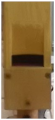 |  |  |  |  | 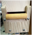 |
|---|---|---|---|---|---|---|---|---|
| Labium type | English bay leaf | Beard | Beard | Beard | Beard | Plate | Roller | Roller |
| Stops | Principal 4ft | Bourdon 8ft | Bourdon 16ft | Dolce Flute 8ft | Flute 4ft | Gamba 8ft | Bass Principal 16ft | Geigen Principal 8ft |
| Construction | Open, pewter (75% tin, 25% lead) | Open, oakwood | Stopped, oakwood | Open, pine | Open, spruce | Open, metal (55% lead, 45% tin) | Open, pine | Open, pine |
| Lip width [mm] | 29.4 | 41.1 | 41.8 | 18.5 | 35.4 | 29 | 108 | 80.5 |
| Internal pipe dimensions [mm] | 37.9 | 41.9 × 51.9 | 42.4 × 54.5 | 19.4 × 29.2 | 35 × 51 | 35.3 | 106 × 140 | 79 × 96 |
| Wavelength [mm] | 530 | 580 | 590 | 290 | 975 | 920 | 2096 | 2471 |
| Distance from the Obstacle | Bourdon 16ft Stopped C Sharp | Bourdon 8ft Open B | Principal 4ft E1 | Gamba 8ft f Sharp | Geigen Principal 8ft Open C | Bass Principal 16ft Open D | Dolce Flute 8ft Open B | Flute 4ft Open D Sharp |
|---|---|---|---|---|---|---|---|---|
| x [mm] | f0 [Hz] | |||||||
| 0 | 131.44 | 238.14 | - | 185.68 | 64.45 | 69.69 | 458.15 | 149.15 |
| 5 | 135.12 | 246.02 | 320.59 | 186.26 | 64.80 | 71.15 | 464.61 | 153.18 |
| 10 | 136.95 | 249.22 | 324.14 | 186.46 | 64.92 | 71.85 | 466.35 | 154.70 |
| 15 | 137.82 | 250.61 | 325.28 | 186.55 | 65.06 | 72.41 | 467.53 | 155.16 |
| 20 | 138.30 | 251.30 | 325.81 | 186.60 | 65.16 | 72.61 | 468.13 | 155.46 |
| 25 | 138.60 | 251.76 | 325.90 | 65.17 | 72.79 | 155.58 | ||
| 30 | 251.99 | 326.16 | 65.22 | 72.98 | 155.68 | |||
| 35 | 252.19 | 326.28 | 65.28 | 73.10 | 155.74 | |||
| 40 | 252.30 | 326.37 | 65.31 | 73.19 | ||||
| 45 | 252.38 | 326.44 | 65.33 | 73.28 | ||||
| 50 | 326.49 | 65.35 | 73.32 | |||||
| 55 | 326.52 | 65.39 | 73.38 | |||||
| 60 | 65.39 | 73.41 | ||||||
| 65 | 65.40 | 73.41 | ||||||
| 70 | 65.45 | 73.26 | ||||||
| 75 | 73.31 | |||||||
| 80 | 73.32 | |||||||
| 85 | 73.34 | |||||||
| x0 (no obstacle) | 139.24 | 252.76 | 327.19 | 186.91 | 65.49 | 73.49 | 469.52 | 155.98 |
| Re | [360, 1300) | [1300, 5000) | [5000, 2 × 10⁵) | [2 × 10⁵, 106) |
| α | 0.2257 | 0.2040 | 0.1776 | 0.5760 |
| τ | −0.4402 | 0.3364 | 2.2023 | −175.956 |
| Re | [2300, 5000) | [5000, 104) | [104, 2 × 10⁵) |
| Sr | (0.2088, 0.211] | (0.1996, 0.2088] | (0.1825, 0.1996] |
| Pipe | Bourdon 16ft Stopped c Sharp | Bourdon 8ft Open b | Principal 4ft e1 | Gamba 8ft F Sharp | Geigen Principal 8ft Open C | Bass Principal 16ft Open D | Dolce Flute 8ft Open B | Flute 4ft Open D Sharp |
|---|---|---|---|---|---|---|---|---|
| f0 [Hz] | 139.240 | 252.76 | 327.2 | 186.91 | 65.49 | 73.49 | 469.52 | 155.98 |
| l [mm] | 16.53 | 15.65 | 7.51 | 8.1 | 15 | 33 | 8 | 12.4 |
| u [m·s−1] | 11.51 | 19.78 | 12.29 | 7.57 | 4.91 | 12.13 | 18.78 | 9.67 |
| Re | 13021 | 21187 | 6315 | 4197 | 5043 | 27389 | 10284 | 8208 |
| Pipe | Bourdon 16ft Stopped c Sharp | Bourdon 8ft Open b | Principal 4ft e1 | Gamba 8ft F Sharp | Geigen Principal 8ft Open C | Bass Principal 16ft Open D | Dolce Flute 8ft Open B | Flute 4ft Open D Sharp |
|---|---|---|---|---|---|---|---|---|
| x0 [mm] | 30 | 50 | 60 | 25 | 75 | 90 | 25 | 40 |
| a [Hz] | 0.91 | 1.76 | 2.14 | 0.13 | 0.12 | 0.45 | 1.32 | 0.83 |
| b [Hz] | 138.37 | 252.50 | 327.35 | 186.65 | 65.36 | 73.39 | 468.16 | 155.83 |
| b2 | 0.994 | 0.999 | 1.001 | 0.999 | 0.998 | 0.999 | 0.997 | 0.999 |
| r2 | 91% | 96% | 85% | 88% | 84% | 90% | 95% | 97% |
Publisher’s Note: MDPI stays neutral with regard to jurisdictional claims in published maps and institutional affiliations. |
© 2021 by the authors. Licensee MDPI, Basel, Switzerland. This article is an open access article distributed under the terms and conditions of the Creative Commons Attribution (CC BY) license (https://creativecommons.org/licenses/by/4.0/).
Share and Cite
Węgrzyn, D.; Wrzeciono, P.; Wieczorkowska, A. The Dependence of Flue Pipe Airflow Parameters on the Proximity of an Obstacle to the Pipe’s Mouth. Sensors 2022, 22, 10. https://doi.org/10.3390/s22010010
Węgrzyn D, Wrzeciono P, Wieczorkowska A. The Dependence of Flue Pipe Airflow Parameters on the Proximity of an Obstacle to the Pipe’s Mouth. Sensors. 2022; 22(1):10. https://doi.org/10.3390/s22010010
Chicago/Turabian StyleWęgrzyn, Damian, Piotr Wrzeciono, and Alicja Wieczorkowska. 2022. "The Dependence of Flue Pipe Airflow Parameters on the Proximity of an Obstacle to the Pipe’s Mouth" Sensors 22, no. 1: 10. https://doi.org/10.3390/s22010010
APA StyleWęgrzyn, D., Wrzeciono, P., & Wieczorkowska, A. (2022). The Dependence of Flue Pipe Airflow Parameters on the Proximity of an Obstacle to the Pipe’s Mouth. Sensors, 22(1), 10. https://doi.org/10.3390/s22010010