
Validation of a Low-Cost Pavement Monitoring Inertial-Based System for Urban Road Networks

 ,
,  , and
, and 
Abstract
1. Introduction
2. Pavement Monitoring Sensors
2.1. General Architecture of the Proposed Sensor
2.1.1. Raspberry Pi Zero W Single-Board Microcomputer
2.1.2. Inertial Measurement Unit
- (1)
- three-axial raw linear accelerations (including gravity) in the sensor frame, in g;
- (2)
- three-axial raw angular velocities in the sensor frame, in rad/s;
- (3)
- three-axial raw magnetic field in the sensor frame, in µT;
- (4)
- pressure, in hPa;
- (5)
- height derived from the barometric calculation, in m;
- (6)
- temperature, in °C;
- (7)
- sensor attitude (roll, pitch, and yaw, in degrees).
2.1.3. Mini Global Positioning System (GPS) Module
2.1.4. Other Components
2.2. LandMark 10 GPSA-150-10-200
2.3. Road Asset Collection System
- the positioning and orientation system (GPS and wheel odometer) so as to georeferenced the data collected with the other on-board sensors;
- on-board sensors (digital camera, DC) for inspection road asset and pavement, n. 5; light detection and ranging (LIDAR) to map roadside equipment and features, n. 2; a laser crack measurement system (LCMS) for automatic inspection of the pavement condition; RSP to collect longitudinal profiles;
- the synchronization system coordinated by a management system.
- the data storage system;
- the power supply system for equipment and documents.
3. Pavement Evaluation Methods
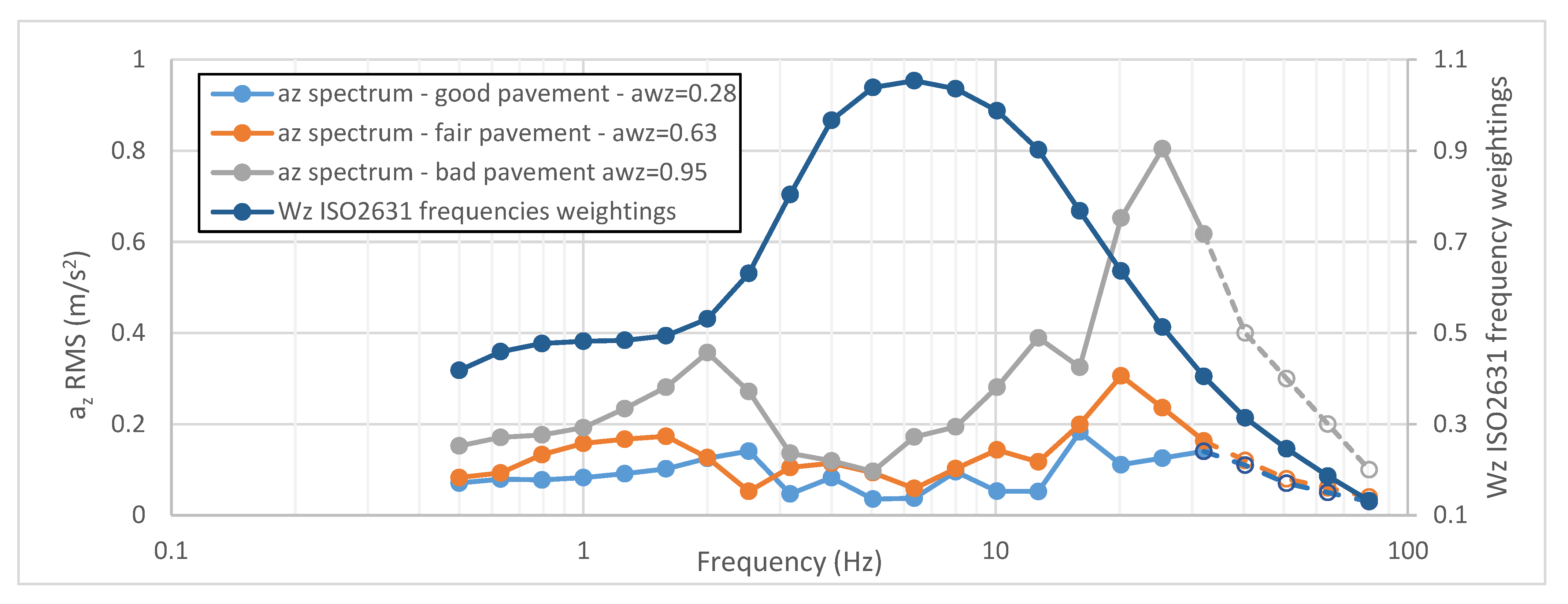
3.1. Whole-Body Vibration—ISO 2631
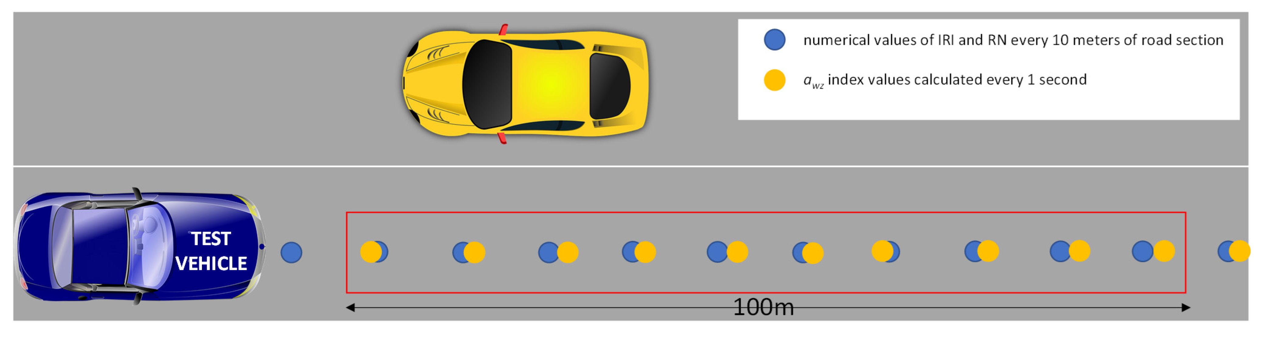
3.2. International Roughness Index (IRI)—ASTM E 1926
3.3. Ride Number RN
4. Field Tests for System Validation
- LandMark 10 GPSA-150-10-200, a precision measuring instrument [75] with sampling frequency equal to 100 Hz. Post-processing acceleration data recorded from this IMU was aimed to obtain the frequency-weighted vertical acceleration awz considering analysis times by one second each;

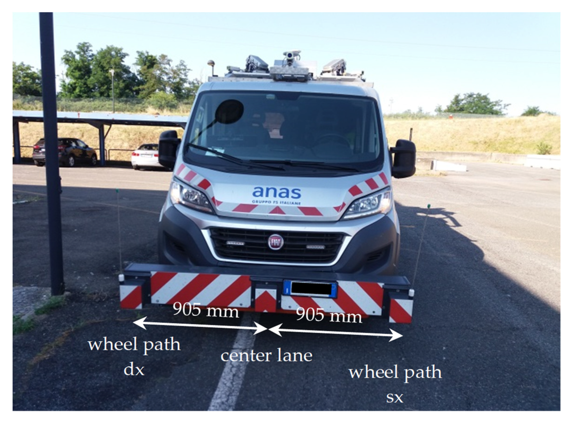
| Test Vehicle | Average Test Speed (km/h) | IMU | IMU Position Inside the Test Vehicle |
|---|---|---|---|
| Renault Zoe 1 | 44 | SENSOR#1 | Passenger side floor (Figure 8a) |
| LandMark | Passenger side floor (Figure 8a) | ||
| Cartesio | 37 | SENSOR#2 | Dashboard (Figure 8b) |
5. Results and Discussion
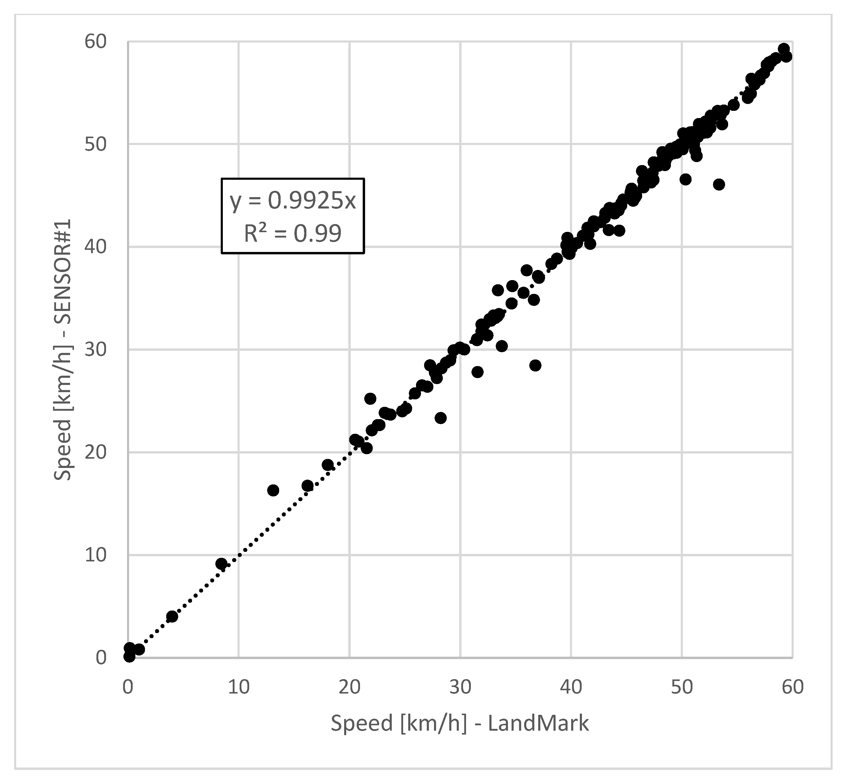
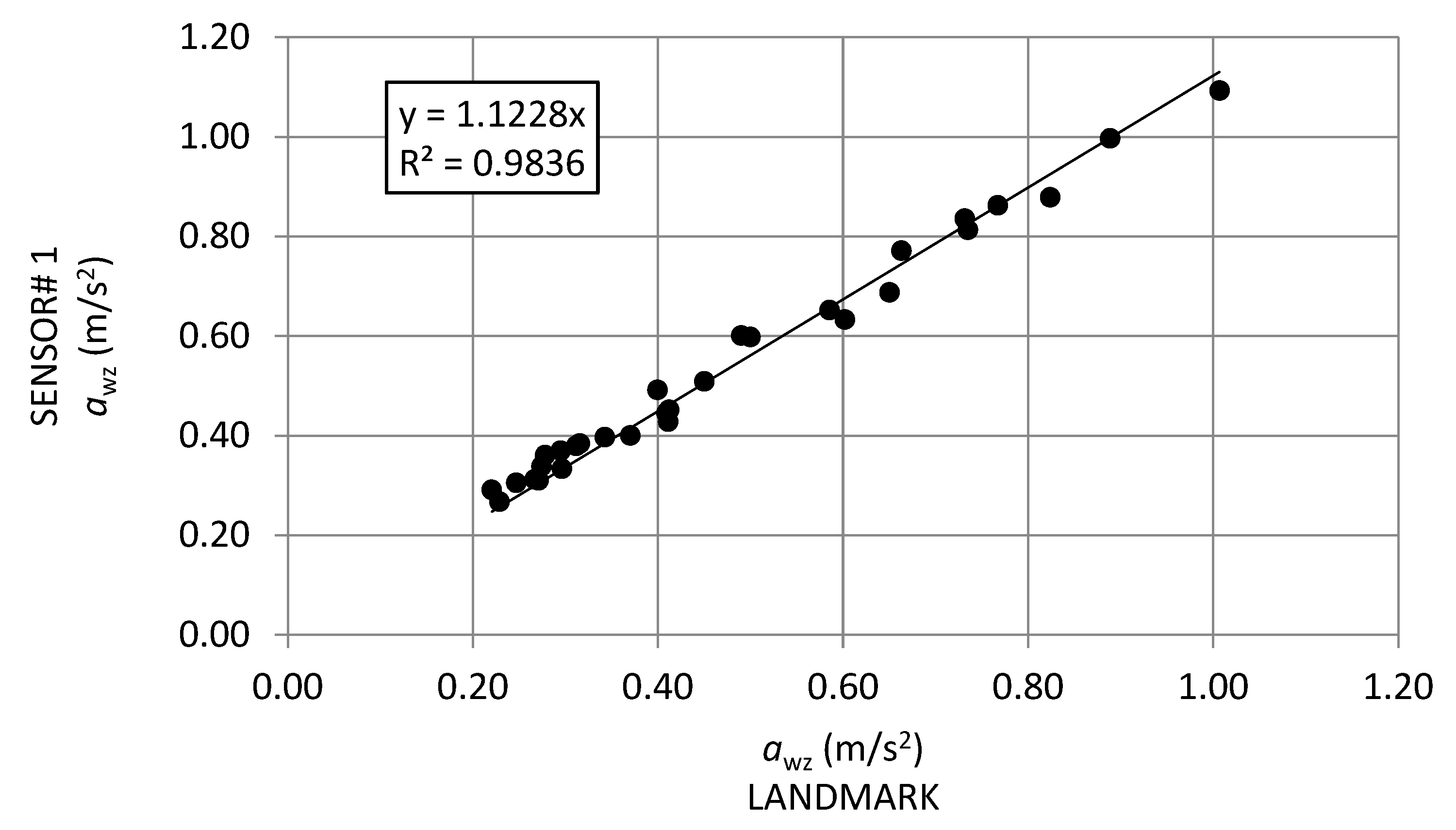
5.1. Comparison between SENSOR#1-awz and LandMark-awz
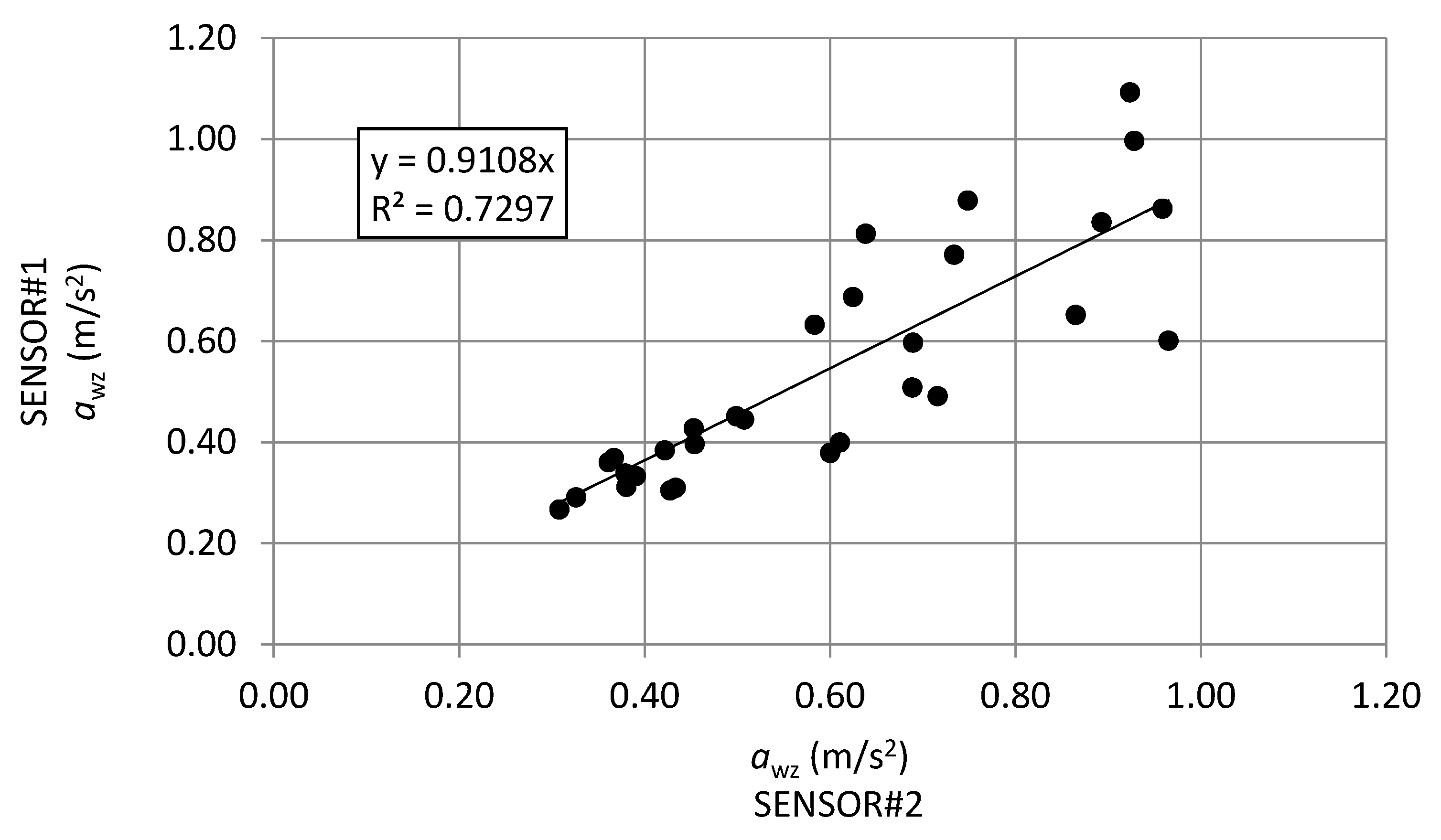
5.2. Comparison between SENSOR#1-awz and SENSOR#2-awz
5.3. Comparison between awz vs. IRI and awz vs. RN
6. Conclusions
Author Contributions
Funding
Institutional Review Board Statement
Informed Consent Statement
Data Availability Statement
Acknowledgments
Conflicts of Interest
References
- Hudson, W.R.; Uddin, W.; Haas, R.C. Infrastructure Management: Integrating Design, Construction, Maintenance, Rehabilitation and Renovation; McGraw-Hill: New York, NY, USA, 1997; ISBN 978-0-07-030895-4. [Google Scholar]
- Uddin, W.; Hudson, W.; Haas, R. Public Infrastructure Asset Management, 2nd ed.; McGraw-Hill Education: New York, NY, USA, 2013; ISBN 0071820124. [Google Scholar]
- Bonin, G.; Polizzotti, S.; Loprencipe, G.; Folino, N.; Oliviero Rossi, C.; Teltayev, B.B. Development of a road asset management system in kazakhstan. In Transport Infrastructure and Systems, Proceedings of the AIIT International Congress on Transport Infrastructure and Systems, Rome, Italy, 10–12 April 2017; CRC Press: Leiden, The Netherlands, 2017; pp. 537–545. ISBN 9781138030091. [Google Scholar]
- Kulkarni, R.B.; Miller, R.W. Pavement Management Systems: Past, Present, and Future. Transp. Res. Rec. 2003, 1853, 65–71. [Google Scholar] [CrossRef]
- Zaabar, I.; Chatti, K. Estimating vehicle operating costs caused by pavement surface conditions. Transp. Res. Rec. 2014, 2455, 63–76. [Google Scholar] [CrossRef]
- Wang, T.; Harvey, J.; Lea, J.; Kim, C. Impact of pavement roughness on vehicle free-flow speed. J. Transp. Eng. 2014, 140, 1–52. [Google Scholar] [CrossRef]
- Múčka, P. Vibration Dose Value in Passenger Car and Road Roughness. J. Transp. Eng. Part B Pavements 2020, 146, 04020064. [Google Scholar] [CrossRef]
- Popoola, M.O.; Apampa, O.A.; Adekitan, O. Impact of Pavement Roughness on Traffic Safety under Heterogeneous Traffic Conditions. Niger. J. Technol. Dev. 2020, 17, 13–19. [Google Scholar] [CrossRef]
- Alfonso, M.O.; Figuero, M.; Velosa, C.N. Alfonso Daniel Effect of road quality on fuel consumption and the generation of externalities derived from transport. Case of study: Barranquilla, Colombia. Espacios 2020, 41, 5. [Google Scholar]
- Li, T. Influencing parameters on tire–pavement interaction noise: Review, experiments, and design considerations. Designs 2018, 2, 38. [Google Scholar] [CrossRef]
- Cantisani, G.; Fascinelli, G.; Loprencipe, G. Urban Road Noise: The Contribution of Pavement Discontinuities. In Proceedings of the ICSDEC 2012: Developing the Frontier of Sustainable Design, Engineering, and Construction, Fort Worth, TX, USA, 7–9 November 2012; pp. 327–334. [Google Scholar]
- Loprencipe, G.; Zoccali, P. Ride quality due to road surface irregularities: Comparison of different methods applied on a set of real road profiles. Coatings 2017, 7, 59. [Google Scholar] [CrossRef]
- Papageorgiou, G. Appraisal of road pavement evaluation methods. J. Eng. Sci. Technol. Rev. 2019, 12, 158–166. [Google Scholar] [CrossRef]
- Shtayat, A.; Moridpour, S.; Best, B.; Shroff, A.; Raol, D. A review of monitoring systems of pavement condition in paved and unpaved roads. J. Traffic Transp. Eng. 2020, 7, 629–638. [Google Scholar]
- Wambold, J.C. The measurement and data analysis used to evaluate highway roughness. Wear 1979, 57, 117–125. [Google Scholar] [CrossRef]
- Múčka, P. Current approaches to quantify the longitudinal road roughness. Int. J. Pavement Eng. 2016, 17, 659–679. [Google Scholar] [CrossRef]
- Sayers, M.W.; Karamihas, S.M. The Little Book of Profiling; The Regent of the University of Michigan: Ann Arbor, MI, USA, 1998. [Google Scholar]
- Chen, D.; Hildreth, J.; Mastin, N. Determination of IRI Limits and Thresholds for Flexible Pavements. J. Transp. Eng. Part B Pavements 2019, 145, 04019013. [Google Scholar] [CrossRef]
- Tehrani, S.S.; Cowe Falls, L.; Mesher, D. Road users’ perception of roughness and the corresponding IRI threshold values. Can. J. Civ. Eng. 2015, 42, 233–240. [Google Scholar] [CrossRef]
- Chen, X.; Zhu, H.; Dong, Q.; Huang, B. Optimal thresholds for pavement preventive maintenance treatments using LTPP data. J. Transp. Eng. 2017, 143, 04017018. [Google Scholar] [CrossRef]
- Múčka, P. Road Roughness Limit Values Based on Measured Vehicle Vibration. J. Infrastruct. Syst. 2017, 23, 04016029. [Google Scholar] [CrossRef]
- Yu, J.; Chou, E.Y.J.; Yau, J.-T. Development of Speed-Related Ride Quality Thresholds Using International Roughness Index. Transp. Res. Rec. J. Transp. Res. Board 2006, 1974, 47–53. [Google Scholar] [CrossRef]
- Loprencipe, G.; Zoccali, P.; Cantisani, G. Effects of vehicular speed on the assessment of pavement road roughness. Appl. Sci. 2019, 9, 1783. [Google Scholar] [CrossRef]
- Gong, J.; Zhou, H.; Gordon, C.; Jalayer, M. Mobile terrestrial laser scanning for highway inventory data collection. In Proceedings of the Congress on Computing in Civil Engineering, Clearwater Beach, FL, USA, 17–20 June 2012; pp. 545–552. [Google Scholar]
- Madeira, S.; Gonçalves, J.A.; Bastos, L. Sensor integration in a low cost land mobile mapping system. Sensors 2012, 12, 2935–2953. [Google Scholar] [CrossRef]
- Rajamohan, D.; Gannu, B.; Rajan, K.S. MAARGHA: A prototype system for road condition and surface type estimation by fusing multi-sensor data. ISPRS Int. J. Geo-Inf. 2015, 4, 1225–1245. [Google Scholar] [CrossRef]
- Chen, K.; Lu, M.; Fan, X.; Wei, M.; Wu, J. Road condition monitoring using on-board three-axis accelerometer and GPS sensor. In Proceedings of the 2011 6th International ICST Conference on Communications and Networking in China, CHINACOM, Harbin, China, 17–19 August 2011; pp. 1032–1037. [Google Scholar]
- Zang, K.; Shen, J.; Huang, H.; Wan, M.; Shi, J. Assessing and mapping of road surface roughness based on GPS and accelerometer sensors on bicycle-mounted smartphones. Sensors 2018, 18, 914. [Google Scholar] [CrossRef]
- Du, Y.; Liu, C.; Wu, D.; Jiang, S. Measurement of international roughness index by using Z -axis accelerometers and GPS. Math. Probl. Eng. 2014, 2014, 1–10. [Google Scholar]
- González, A.; O’Brien, E.J.; Li, Y.Y.; Cashell, K. The use of vehicle acceleration measurements to estimate road roughness. Veh. Syst. Dyn. 2008, 46, 483–499. [Google Scholar] [CrossRef]
- Amador-Jiménez, L.; Matout, N. A low cost solution to assess road’s roughness surface condition for Pavement Management. In Proceedings of the Transportation Research Board 93rd Annual Meeting—Compendium of Papers, Washington DC, USA, 12–16 January 2014; Volume 2424, p. 16. [Google Scholar]
- Harikrishnan, P.M.; Gopi, V.P. Vehicle Vibration Signal Processing for Road Surface Monitoring. IEEE Sens. J. 2017, 17, 5192–5197. [Google Scholar] [CrossRef]
- Islam, S.; Buttlar, W.G.; Aldunate, R.G.; Vavrik, W.R. Measurement of pavement roughness using android-based smartphone application. Transp. Res. Rec. 2014, 2457, 30–38. [Google Scholar] [CrossRef]
- Strazdins, G.; Mednis, A.; Kanonirs, G.; Zviedris, R.; Selavo, L. Towards Vehicular Sensor Networks with Android Smartphones for Road Surface Monitoring. In Proceedings of the Second International Workshop on Networks of Cooperating Objects (CONET), Chicago, IL, USA, 11 April 2011; pp. 1–4. [Google Scholar]
- Douangphachanh, V.; Oneyama, H. Exploring the use of smartphone accelerometer and gyroscope to study on the estimation of road surface roughness condition. In Proceedings of the ICINCO 2014—11th International Conference on Informatics in Control, Automation and Robotics, Vienna, Austria, 1–3 September 2014; Volume 1, pp. 783–787. [Google Scholar]
- Douangphachanh, V.; Oneyama, H. Using Smartphones to Estimate Road Pavement Condition. In Proceedings of the International Symposium of Next Generation Infrastructure, Wollongong, Australia, 1–4 October 2013; Campbell, P., Perez, P., Eds.; SMART Infrastructure Facility, University of Wollongong: Wollongong, Australia, 2014. [Google Scholar]
- Tai, Y.; Chan, C.; Hsu, J.Y. Automatic Road Anomaly Detection Using Smart Mobile Device. In Proceedings of the 2010 Conference on Technologies and Applications of Artificial Intelligence (TAAI2010), Hsinchu City, Taiwan, 18–20 November 2010. [Google Scholar]
- Vittorio, A.; Vittoria, C.M.; Guido, D.; Demetrio, C.F.; Vincenzo, P.G.; Iuele, T.; Rosolino, V. A mobile application for road surface quality control: UNIquALroad. Procedia Soc. Behav. Sci. 2012, 54, 1135–1144. [Google Scholar]
- Singh, G.; Bansal, D.; Sofat, S.; Aggarwal, N. Smart patrolling: An efficient road surface monitoring using smartphone sensors and crowdsourcing. Pervasive Mob. Comput. 2017, 40, 71–88. [Google Scholar] [CrossRef]
- Forslöf, L.; Jones, H. Roadroid: Continuous Road Condition Monitoring with Smart Phones. J. Civ. Eng. Arch. 2015, 9, 485–496. [Google Scholar] [CrossRef]
- Alessandroni, G.; Klopfenstein, L.C.; Delpriori, S.; Dromedari, M.; Luchetti, G.; Paolini, B.D.; Seraghiti, A.; Lattanzi, E.; Freschi, V.; Carini, A.; et al. SmartRoadSense: Collaborative road surface condition monitoring. In Proceedings of the UBICOMM 2014—8th International Conference on Mobile Ubiquitous Computing, Systems, Services and Technologies, Rome, Italy, 24–28 August 2014; pp. 210–215. [Google Scholar]
- Lima, L.C.; Amorim, V.J.P.; Pereira, I.M.; Ribeiro, F.N.; Oliveira, R.A.R. Using crowdsourcing techniques and mobile devices for asphaltic pavement quality recognition. In Proceedings of the Brazilian Symposium on Computing System Engineering, SBESC, João Pessoa, Brazil, 1–4 November 2016; pp. 144–149. [Google Scholar]
- Cantisani, G.; Loprencipe, G. Road Roughness and Whole Body Vibration: Evaluation Tools and Comfort Limits. J. Transp. Eng. 2010, 136, 818–826. [Google Scholar] [CrossRef]
- Múčka, P. International Roughness Index specifications around the world. Road Mater. Pavement Des. 2017, 18, 929–965. [Google Scholar] [CrossRef]
- Abudinen, D.; Fuentes, L.G.; Muñoz, J.S.C. Travel quality assessment of urban roads based on international roughness index: Case study in Colombia. Transp. Res. Rec. 2017, 2612, 1–10. [Google Scholar] [CrossRef]
- La Torre, F.; Ballerini, L.; Di Volo, N. Correlation between longitudinal roughness and user perception in urban areas. Transp. Res. Rec. 2002, 1806, 131–139. [Google Scholar] [CrossRef]
- Kırbaş, U.; Karaşahin, M. Investigation of ride comfort limits on urban asphalt concrete pavements. Int. J. Pavement Eng. 2018, 19, 949–955. [Google Scholar] [CrossRef]
- Fichera, G.; Scionti, M.; Garescì, F. Experimental Correlation between the Road Roughness and the Comfort Perceived in Bus Cabins; SAE: Warrendale, PA, USA, 2007. [Google Scholar]
- Ahlin, K.; Granlund, N.O.J. Relating Road Roughness and Vehicle Speeds to Human Whole Body Vibration and Exposure Limits. Int. J. Pavement Eng. 2002, 3, 207–216. [Google Scholar] [CrossRef]
- Ahlin, K.; Granlund, J. International roughness index, IRI, and ISO 2631 vibration evaluation. Transp. Res. Board Comm. Surf. Prop. 2001, 6, 7. [Google Scholar]
- Raspberry Pi Foundation. Raspberry Pi Zero W—Technical Specifications. Available online: https://www.raspberrypi.org/products/raspberry-pi-zero-w/ (accessed on 29 March 2021).
- International Organization for Standardization. ISO2631-1: Mechanical Vibration and Shock—Evaluation of Human Exposure to Whole-Body Vibration—Part 1: General Requirements; International Organization for Standardization: Geneva, Switzerland, 1997. [Google Scholar]
- ASTM International. E950M-09(2018): Standard Test Method for Measuring the Longitudinal Profile of Traveled Surfaces with an Accelerometer-Established Inertial Profiling Reference; ASTM International: West Conshohocken, PA, USA, 2018. [Google Scholar]
- Titterton, D.; Weston, J. Strapdown Inertial Navigation Technology; Institution of Engineering and Technology: London, UK, 2004; ISBN 9780863413582. [Google Scholar]
- InvenSense. MPU-9250 Product Specification Revision 1.1; InvenSense: San Jose, CA, USA, 2019. [Google Scholar]
- Bosch. BMP280: Datasheet. Digit. Presusure Sens; Bosch: Gerlingen, Germany, 2015. [Google Scholar]
- Richards Tech RTIMULib2—A Versatile C++ and Python 9-dof, 10-dof and 11-dof IMU Library GitHub—RTIMULib/RTIMULib2. Available online: https://github.com/RTIMULib/RTIMULib2 (accessed on 29 March 2021).
- Modules, U.N.-6 u-blox 6 G. Available online: https://www.U-Blox.com (accessed on 29 March 2021).
- van Diggelen, F. A-GPS: Assisted GPS, GNSS, and SBAS; Artech Housh: Norwood, MA, USA, 2009; 400p. [Google Scholar]
- Hofmann-Wellenhof, B.; Lichtenegger, H.; Wasle, E. GNSS—GPS, GLONAS, GALILEO and More; Springer: Berlin/Heidelberg, Germany, 2008; ISBN 9783211730126. [Google Scholar]
- Braam, M.P.G. Client—A Library for Polling Gpsd in P. GitHub—MartijnBraam/gpsd-py3: Python 3 GPSD Client. Available online: https://github.com/MartijnBraam/gpsd-py3 (accessed on 29 March 2021).
- Gladiator Technologies Web Page. Available online: https://gladiatortechnologies.com/ (accessed on 29 March 2021).
- GLAMR Software Web Page. Available online: https://gladiatortechnologies.com/software-development-kit/ (accessed on 29 March 2021).
- ANAS Web Site. Available online: https://www.stradeanas.it/it (accessed on 29 March 2021). (In Italian).
- FS GROUP Group Companies Web Site. Available online: https://www.fsitaliane.it/content/fsitaliane/en/fs-group/group-companies.html (accessed on 29 March 2021).
- International Organization for Standardization. ISO:8608-2016: Mechanical Vibration—Road Surface Profiles—Reporting of Measured Data; International Organization for Standardization: Geneva, Switzerland, 2016. [Google Scholar]
- International Organization for Standardization. ISO:13473-4:2008. Characterization of Pavement Texture by Use of Surface Profiles—Part 4: Spectral Analysis of Surface Profiles; International Organization for Standardization: Geneva, Switzerland, 2008. [Google Scholar]
- Yang, W.Y. Signals and Systems with Matlab; Springer: Heidelberg, Germany, 2009; ISBN 9783540929536. [Google Scholar]
- Sayers, M.W. On the Calculation of International Roughness Index from Longitudinal Road Profile; Transportation Research Board: Washington, DC, USA, 1995; pp. 1–12. [Google Scholar]
- Chen, C.; Zhang, J. Comparisons of IRI-Based Pavement Deterioration Prediction Models Using New Mexico Pavement Data. In Proceedings of the Geo-Frontiers Congress 2011, Dallas, TX, USA, 13–16 March 2011; pp. 4594–4603. [Google Scholar]
- Al-Suleiman, T.I.; Shiyab, A.M.S. Prediction of Pavement Remaining Service Life Using Roughness Data—Case Study in Dubai. Int. J. Pavement Eng. 2003, 4, 121–129. [Google Scholar] [CrossRef]
- ASTM International. ASTME1926:08. Standard Practice for Computing International Roughness Index of Roads from Longitudinal Profile Measurements; ASTM International: West Conshohocken, PA, USA, 2013; pp. 1–16. [Google Scholar]
- Janoff, M.S.; Nick, J.B.; Davit, P.S.; Hayhoe, G.F. Pavement Roughness and Rideability; National Research Council: Washington, DC, USA, 1985. [Google Scholar]
- ASTM International. ASTM E1489—98. Standard Practice for Computing Ride Number of Roads from Longitudinal Profile Measurements Made by an Inertial Profile Measuring Device; ASTM International: West Conshohocken, PA, USA, 1998. [Google Scholar]
- Zoccali, P.; Loprencipe, G.; Lupascu, R.C. Acceleration measurements inside vehicles: Passengers’ comfort mapping on railways. Meas. J. Int. Meas. Confed. 2018, 129, 489–498. [Google Scholar] [CrossRef]
- Pavetesting (UK) PaveProf V2.0. Available online: https://pavetesting.com/profiling-and-digital-imaging/ (accessed on 29 March 2021).
- Abulizi, N.; Kawamura, A.; Tomiyama, K.; Fujita, S. Measuring and evaluating of road roughness conditions with a compact road profiler and ArcGIS. J. Traffic Transp. Eng. 2016, 3, 398–411. [Google Scholar] [CrossRef]
- Cafiso, S.; Di Graziano, A. Definition of Homogenous Sections in Road Pavement Measurements. Procedia Soc. Behav. Sci. 2012, 53, 1069–1079. [Google Scholar] [CrossRef]


| Property | Accelerometer | Gyroscope | Magnetometer |
|---|---|---|---|
| Full-scale range | User-programmable: +− 2, 4, 8 or 16 g | User-programmable: 250, 500, 1000 or 2000 °/s | +− 4800 µT |
| Noise spectral density | 300 µg/√Hz | 0.01 °/s/√Hz | - |
| Sensitivity scale factor | User programmable: 16,384, 8192, 4096 or 2048 LBS/g | User-programmable: 131, 65.5, 32.8 or 16.4 LBS/(°/s)) | 0.6 µT/LSB |
| Sample rate | up to 4000 Hz | up to 8000 Hz | up to 8 Hz |
| SBAS | Wide Area Augmentation System, European Geostationary Navigation Overlay Service, and Multi-functional Satellite Augmentation System |
| Maximum update rate | 5 Hz |
| Time-To-First-Fix 1 | Cold or warm start: 27 s Hot start: 2 s Aided start: < 3 s |
| Horizontal position error 2 | GPS: 2.5 m |
| SBAS: 2.0 m | |
| Velocity error 2 | 0.1 m/s |
| Bearing error 2 | 0.5 degree |
| Ride Number | |
|---|---|
| less than 0.315 | Not uncomfortable |
| 0.315–0.63 | Little uncomfortable |
| 0.5–1.0 | Fairly uncomfortable |
| 0.8–1.6 | Uncomfortable |
| 1.25–2.5 | Very uncomfortable |
| more than 2.5 | Extremely uncomfortable |
| Description | Ride Number |
|---|---|
| Perfect | 5.0 |
| Very Good | 4.5 |
| 4.0 | |
| Good | 3.5 |
| 3.0 | |
| Fair | 2.5 |
| 2.0 | |
| Poor | 1.5 |
| 1.0 | |
| Very poor | 0.5 |
| Impassable | 0.0 |
| Branch | Length (m) | Speed Limit (km/h) | Road Classification | Traffic Light (Number) | Priority Road Signs (Number) |
|---|---|---|---|---|---|
| A | 500 | 50 | Urban | NO | NO |
| B | 550 | 30 | Urban | NO | NO |
| C | 100 | 30 | Urban | NO | YES (2) |
| D | 650 | 30 | Urban | NO | YES (1) |
| E | 180 | 30 | Urban | NO | YES (1) |
| F | 2800 | 50 | Urban | NO | YES (1) |
| G | 5700 | 50 | Nonurban | YES (5) | NO |
| H | 230 | 30 | Urban | NO | YES (2) |
| I | 7400 | 50 | Nonurban | NO | YES (1) |
| A | 3600 | 50 | Urban | NO | NO |
| Pavement Condition Category | IRI [mm/m] |
|---|---|
| GOOD | IRI < 3 |
| FAIR | 3–5 |
| POOR | IRI > 5 |
| Section Name | Condition | Chainage (km) | Length (m) | Number of Sub-Sections 1 | |
|---|---|---|---|---|---|
| Start | End | ||||
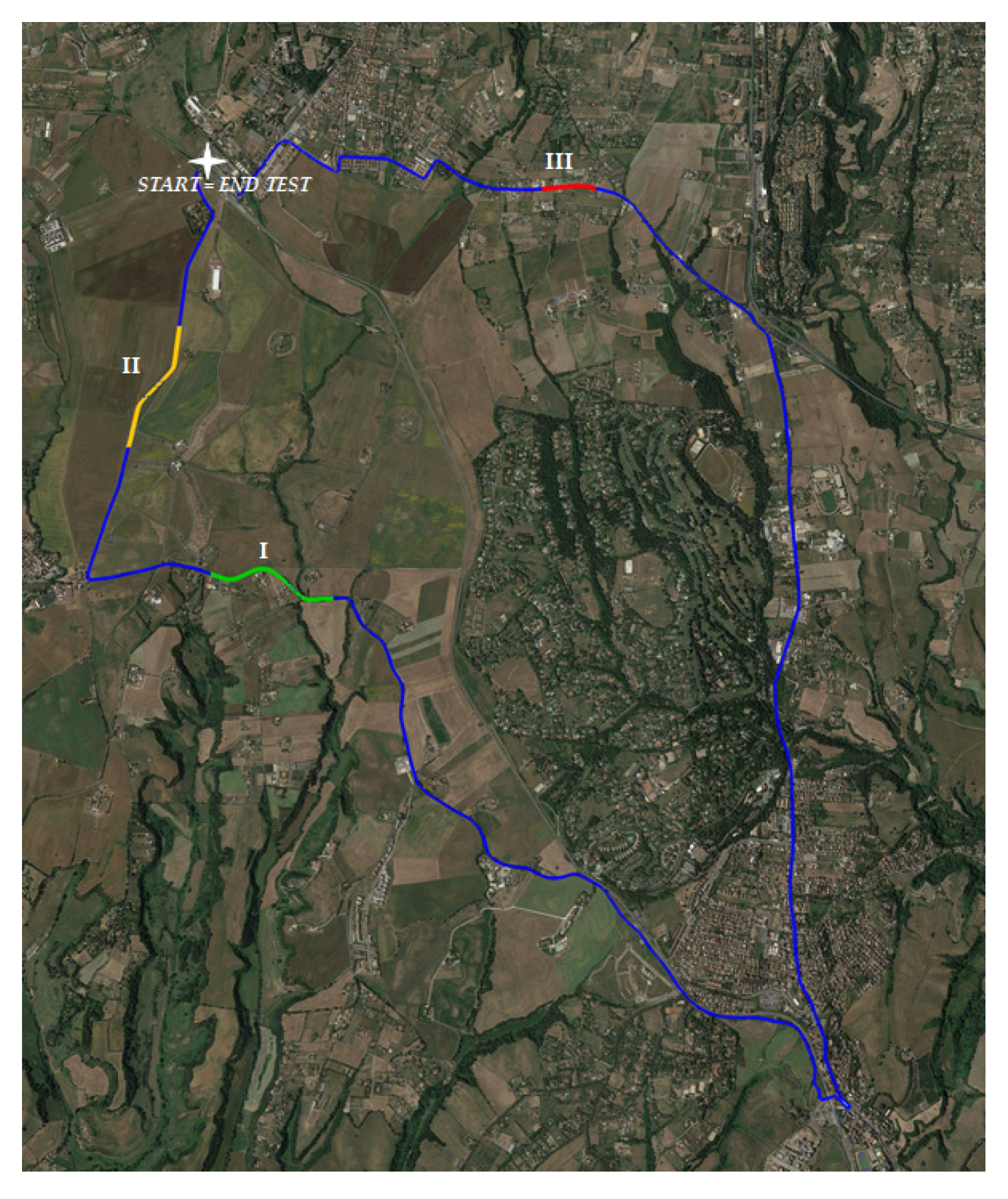
| I | Good | 16 + 300 | 17 + 300 | 1000 | 10 |
| II | Fair | 19 + 200 | 20 + 200 | 1000 | 10 |
| III | Poor | 2 + 800 | 3 + 200 | 400 | 4 |
| 2400 | 24 | ||||
Publisher’s Note: MDPI stays neutral with regard to jurisdictional claims in published maps and institutional affiliations. |
© 2021 by the authors. Licensee MDPI, Basel, Switzerland. This article is an open access article distributed under the terms and conditions of the Creative Commons Attribution (CC BY) license (https://creativecommons.org/licenses/by/4.0/).
Share and Cite
Loprencipe, G.; de Almeida Filho, F.G.V.; de Oliveira, R.H.; Bruno, S. Validation of a Low-Cost Pavement Monitoring Inertial-Based System for Urban Road Networks. Sensors 2021, 21, 3127. https://doi.org/10.3390/s21093127
Loprencipe G, de Almeida Filho FGV, de Oliveira RH, Bruno S. Validation of a Low-Cost Pavement Monitoring Inertial-Based System for Urban Road Networks. Sensors. 2021; 21(9):3127. https://doi.org/10.3390/s21093127
Chicago/Turabian StyleLoprencipe, Giuseppe, Flavio Guilherme Vaz de Almeida Filho, Rafael Henrique de Oliveira, and Salvatore Bruno. 2021. "Validation of a Low-Cost Pavement Monitoring Inertial-Based System for Urban Road Networks" Sensors 21, no. 9: 3127. https://doi.org/10.3390/s21093127
APA StyleLoprencipe, G., de Almeida Filho, F. G. V., de Oliveira, R. H., & Bruno, S. (2021). Validation of a Low-Cost Pavement Monitoring Inertial-Based System for Urban Road Networks. Sensors, 21(9), 3127. https://doi.org/10.3390/s21093127