
Response of Transitional Mixtures Retaining Memory of In-Situ Overburden Pressure Monitored Using Electromagnetic and Piezo Crystal Sensors


Abstract
1. Introduction
2. Theoretical Aspects
2.1. Low- and High-Threshold Fine Fractions
2.2. Void Ratios: Correlations from Soil Index Properties
3. Data Compilation
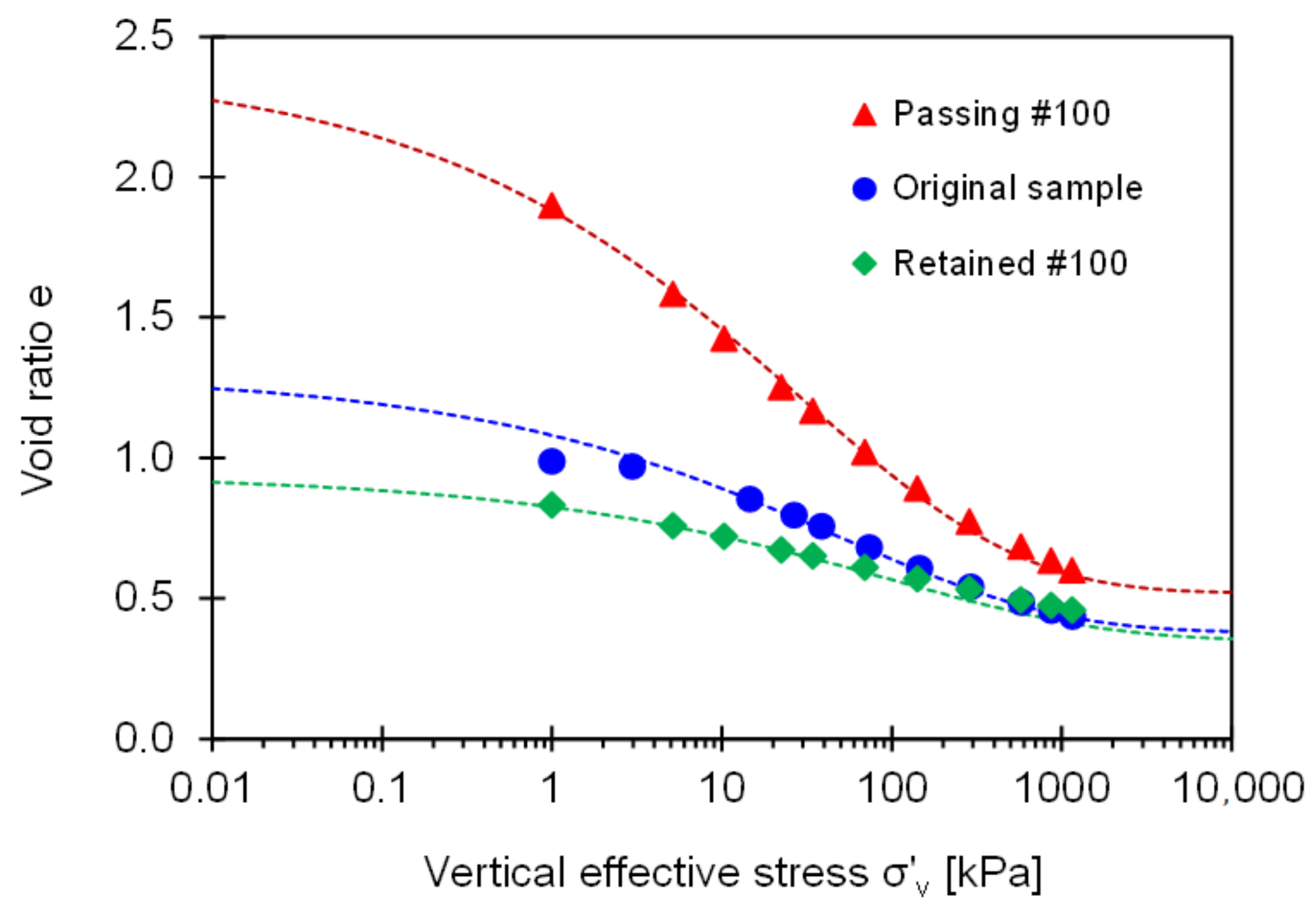
3.1. Void Ratio
3.2. Shear Wave Velocity
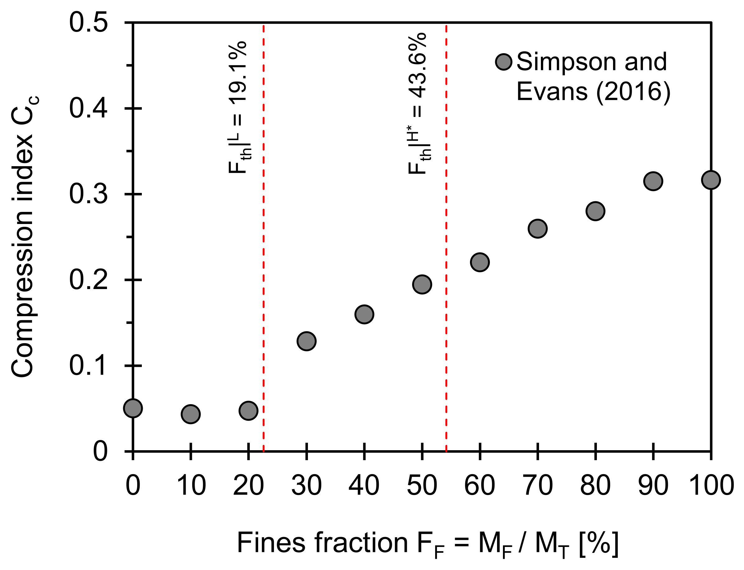
3.3. Compression Index
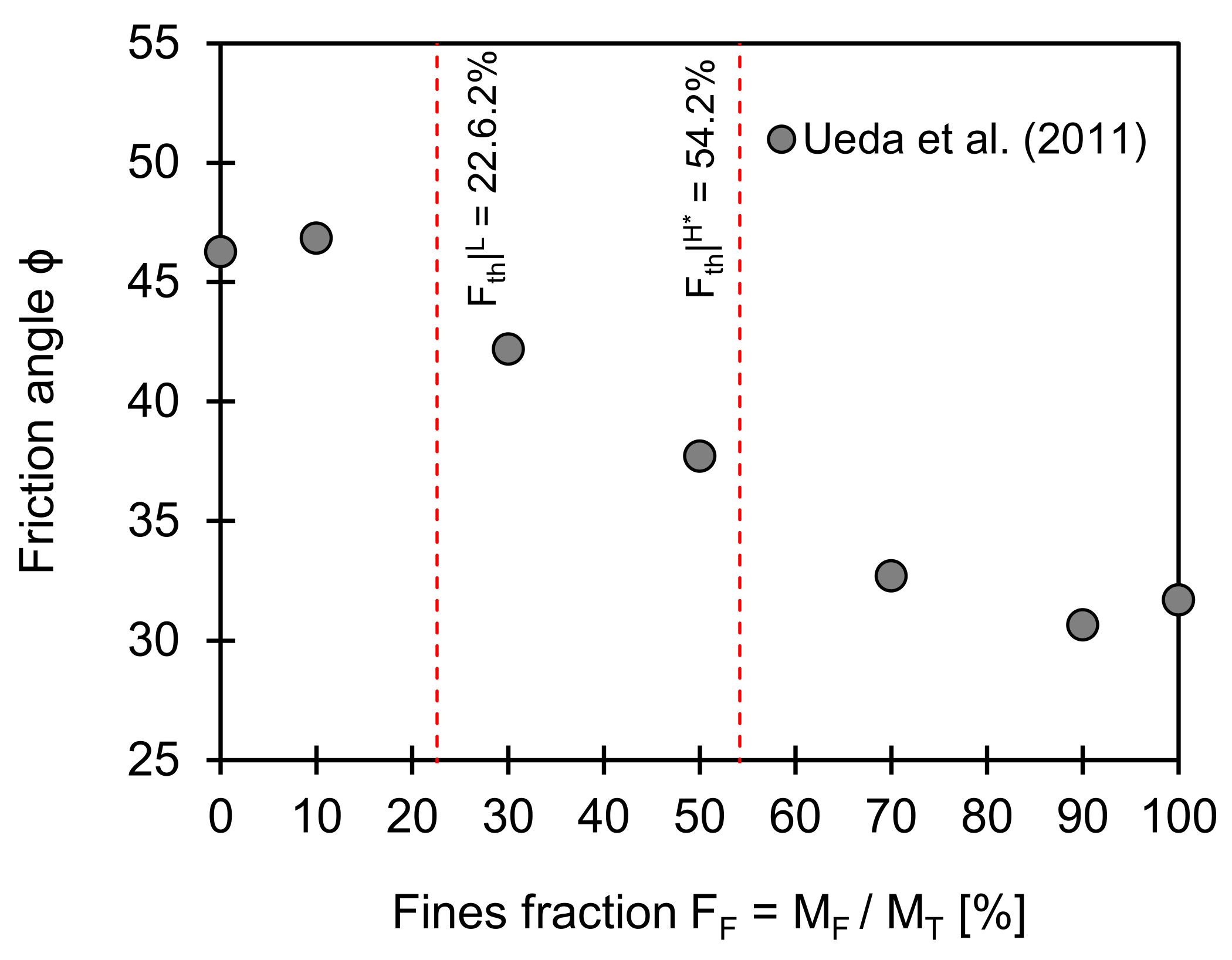
3.4. Friction Angle
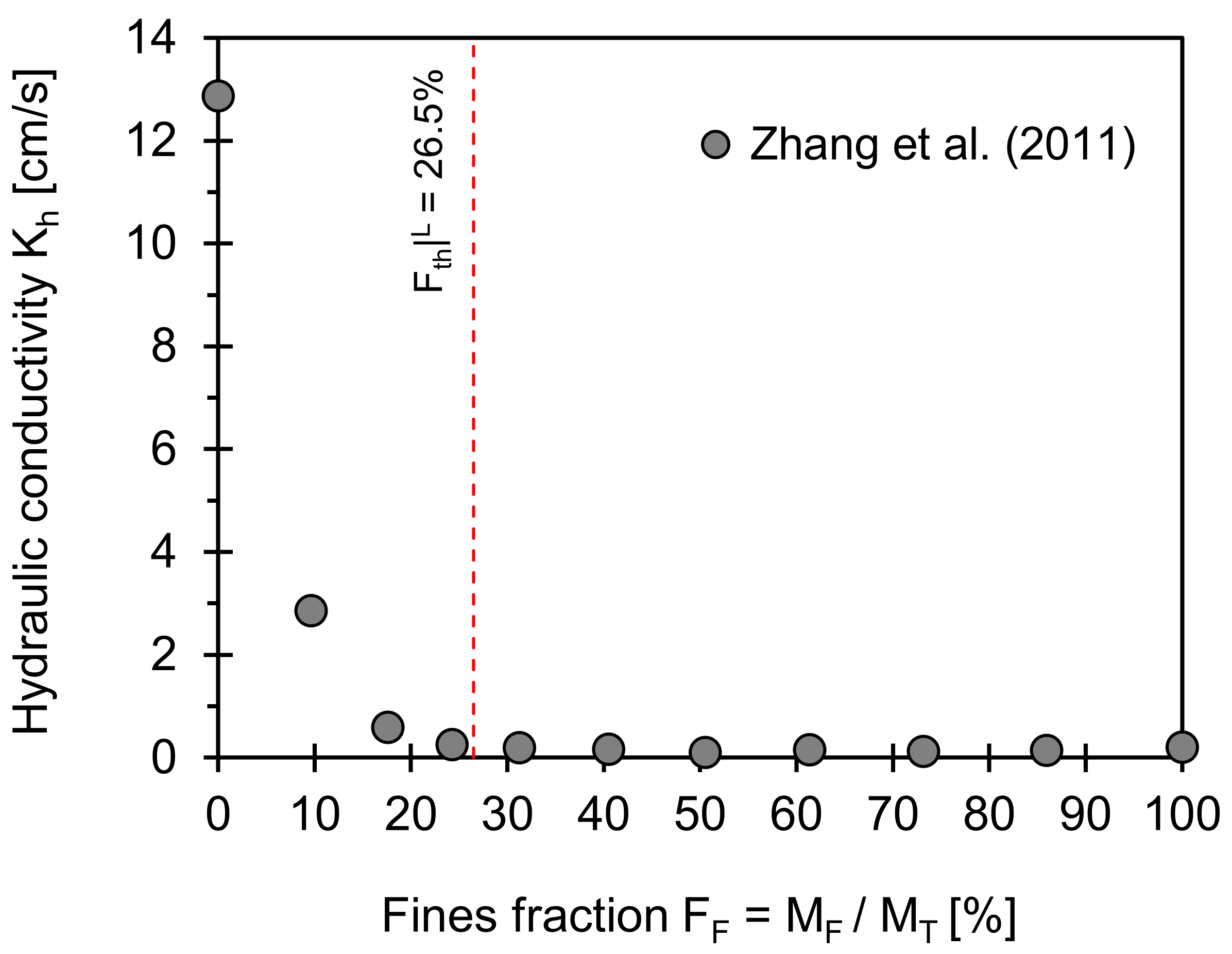
3.5. Hydraulic Conductivity
4. Materials and Methods
4.1. Savannah River Site
4.2. Savannah River Soil: Specimen Preparation
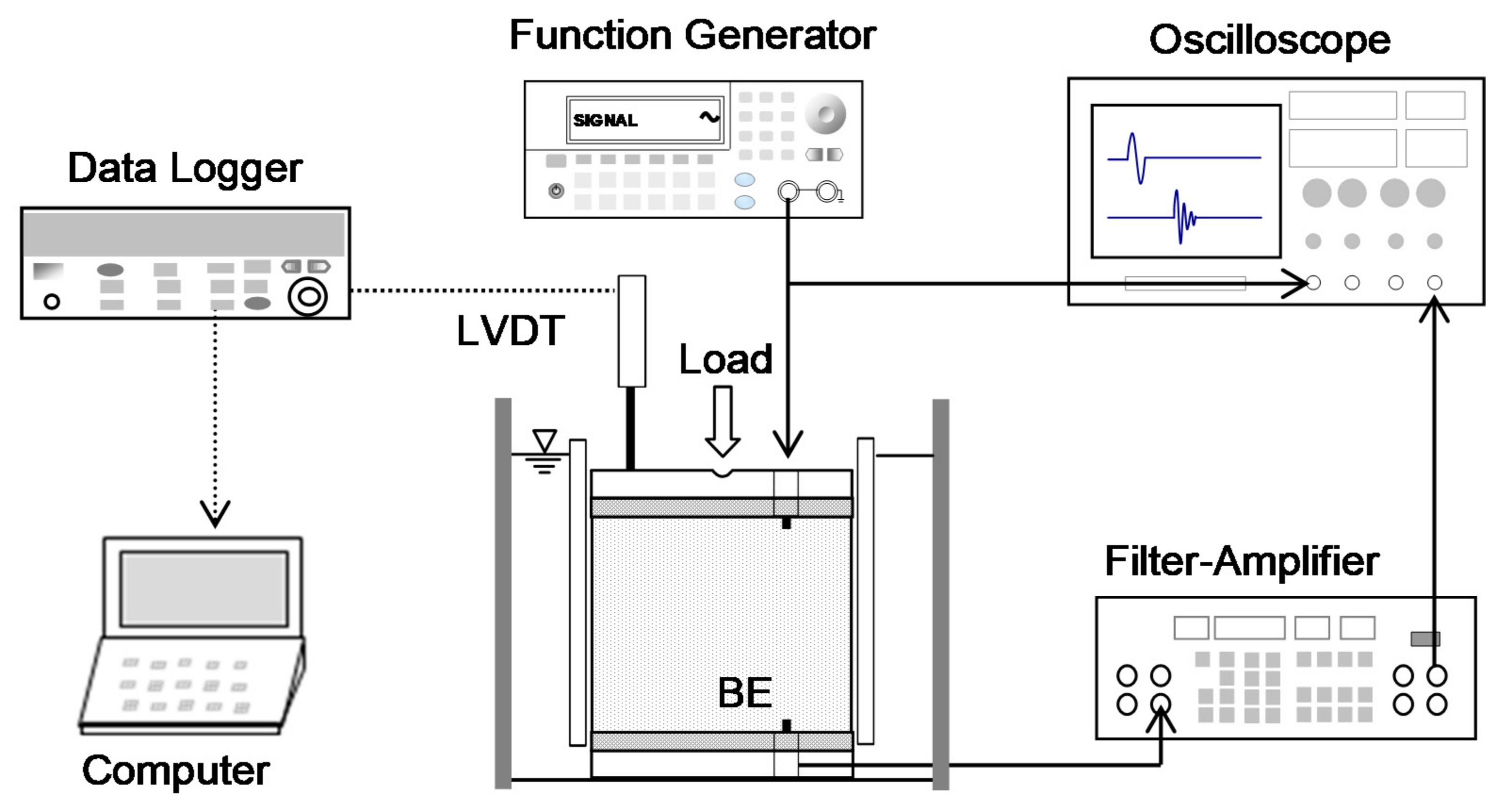
4.3. Instrumented Oedometer Cell
4.4. Deformation and Shear Wave Monitoring
5. Results and Discussion
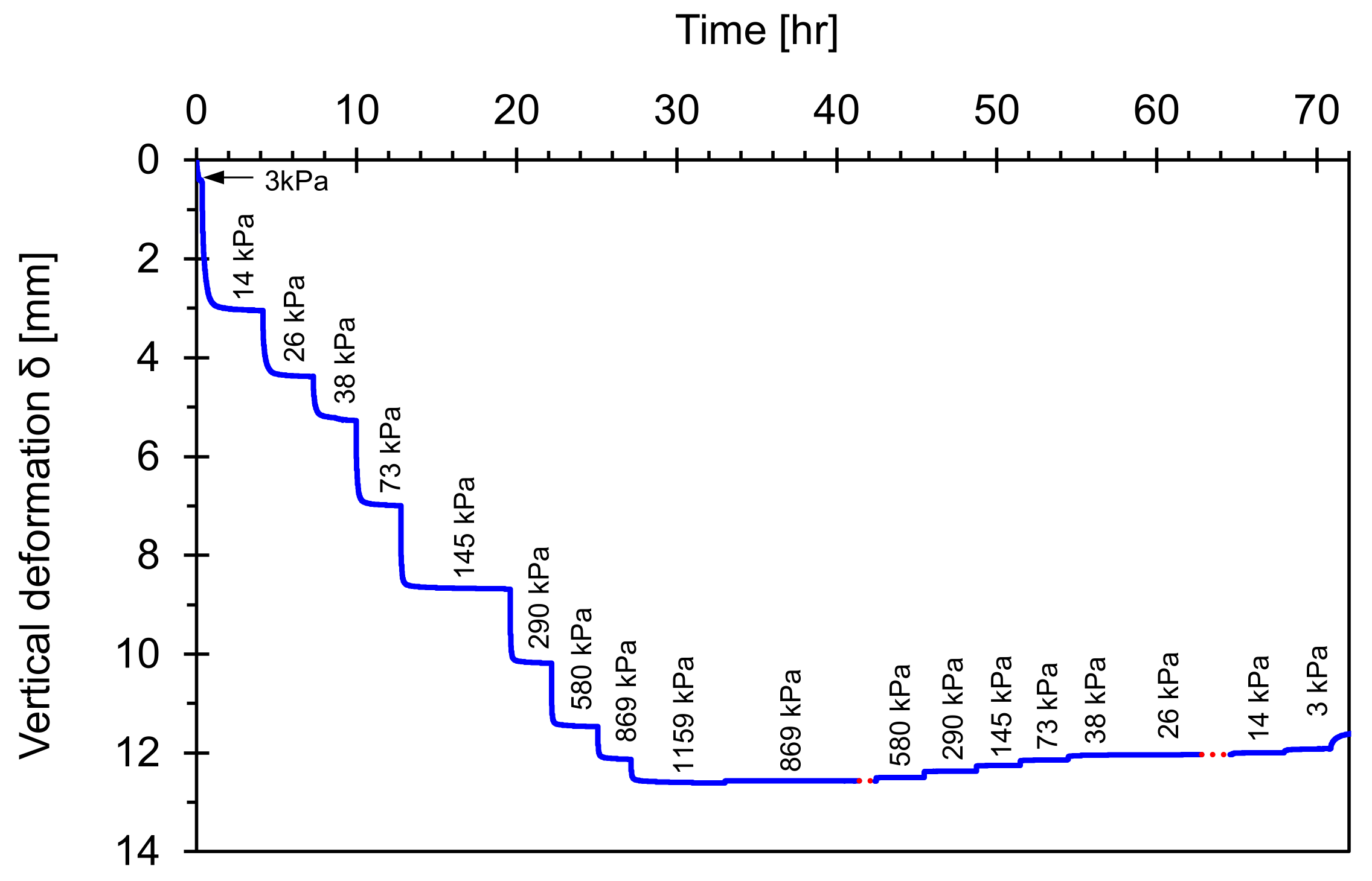
5.1. Vertical Deformation and Void Ratio
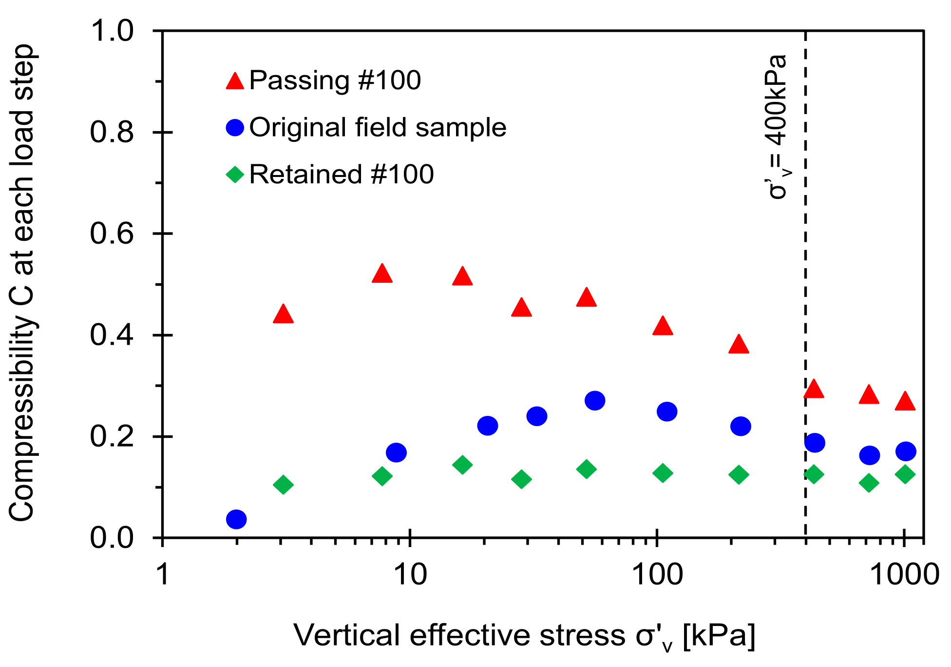
5.2. Compressibility at Each Loading Step (Large Strain)
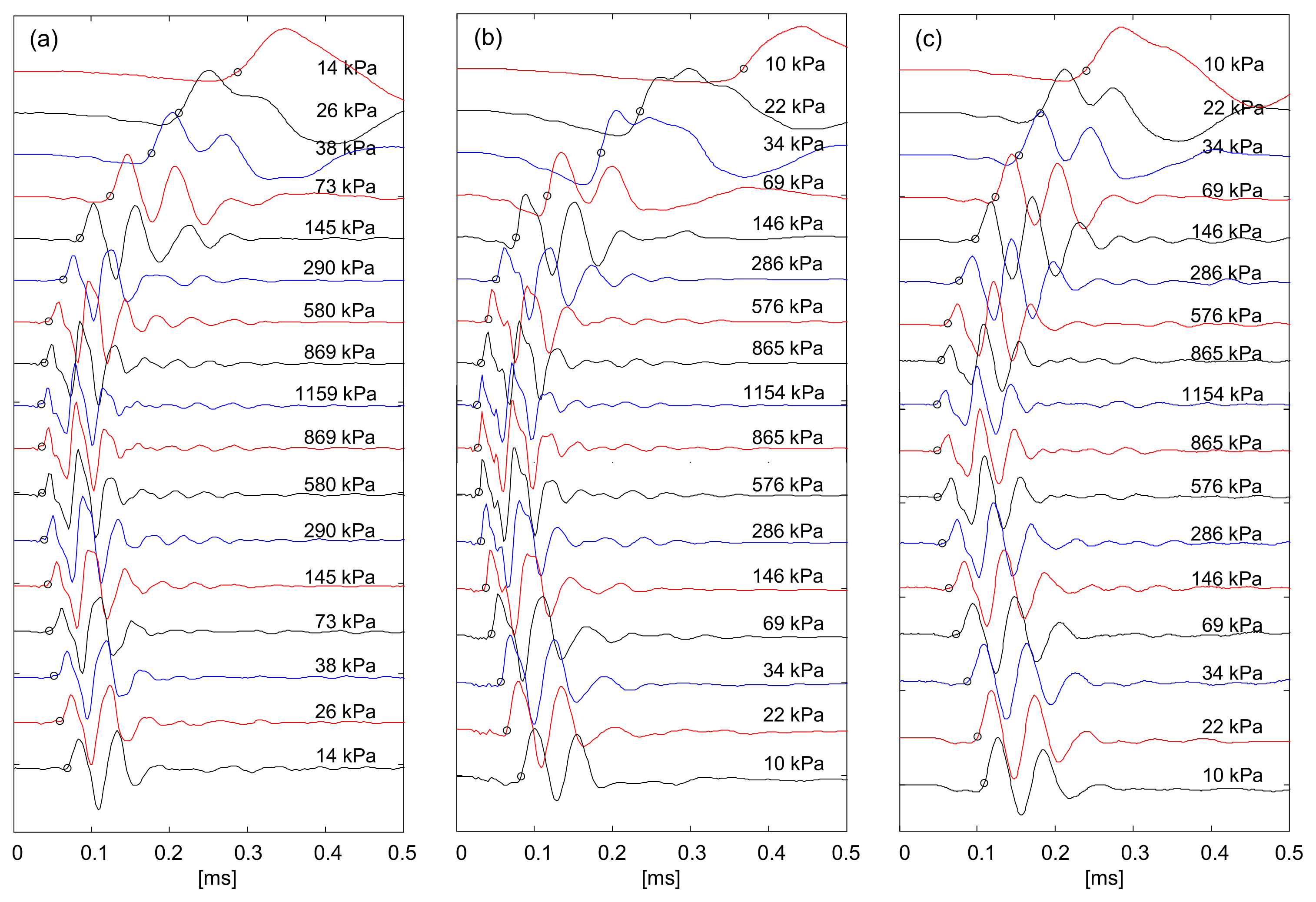
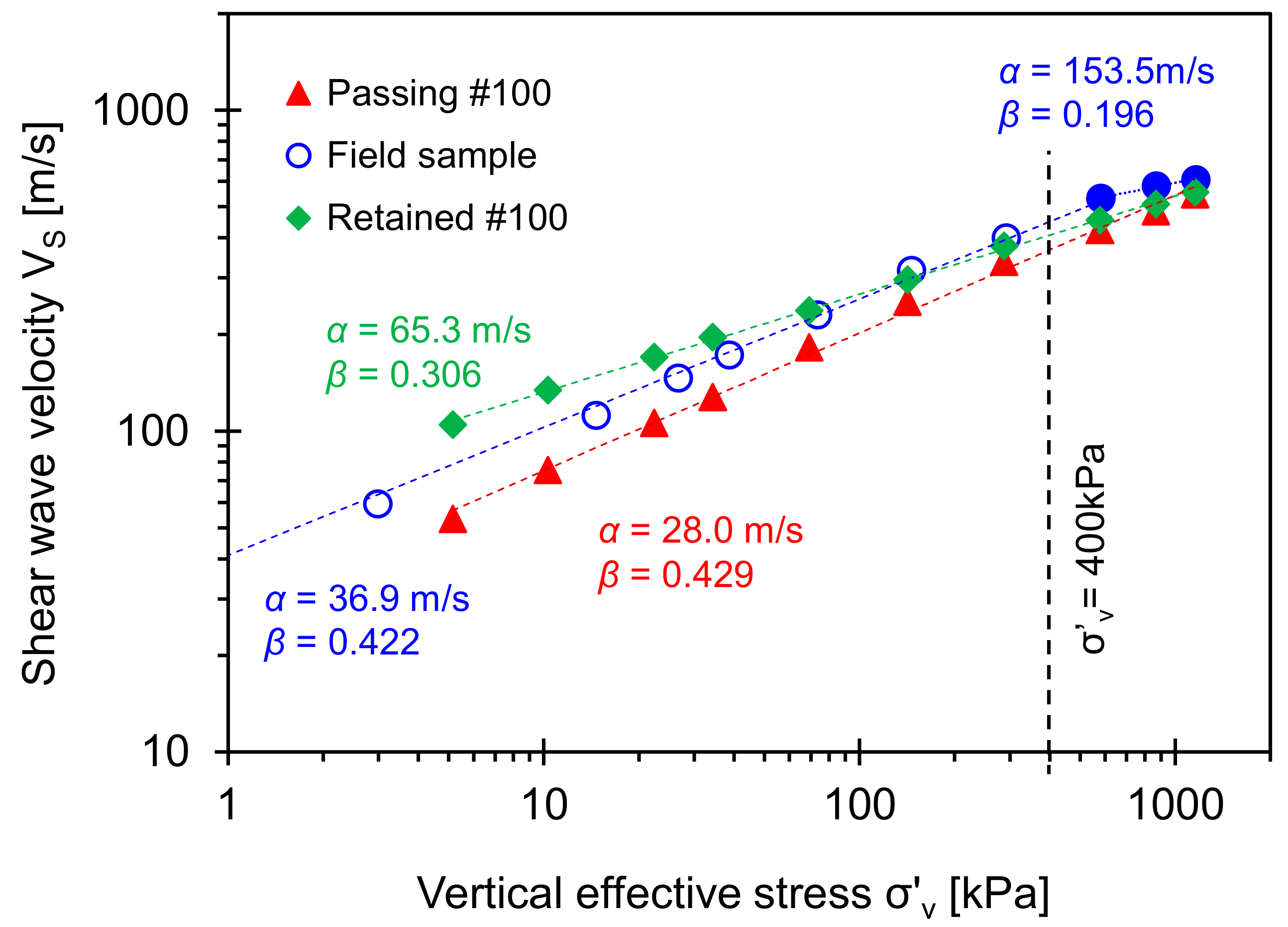
5.3. Shear Wave Velocity (Small Strain)
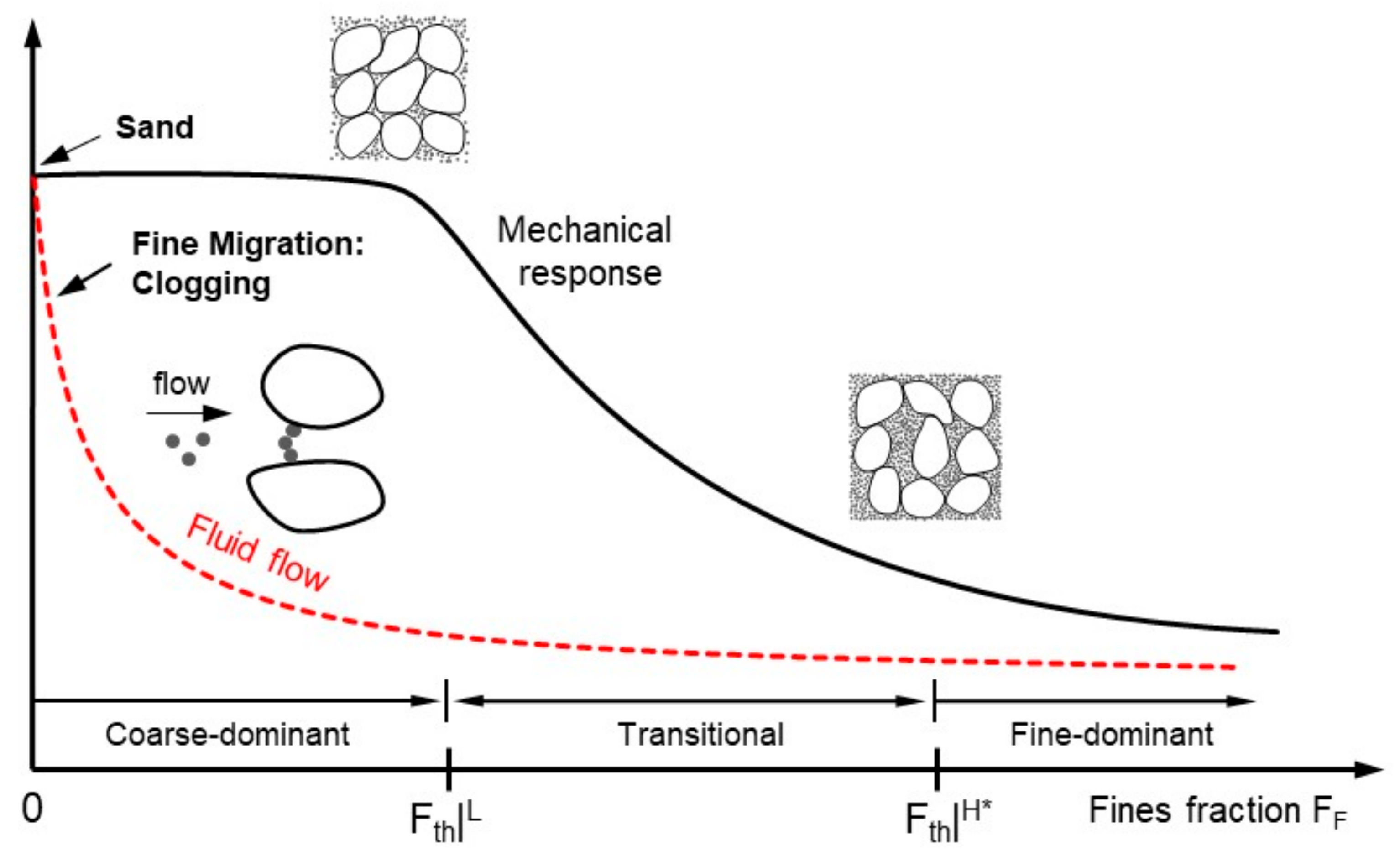
5.4. Fines Migration and Clogging
5.5. New Features of RSCS
6. Conclusions
- Low Fth|L and data-adjusted high Fth|H* threshold fines fractions defined by theoretical volumetric–gravimetric relations successfully capture the transitional behavior in engineering properties (e.g., void ratio, shear wave velocity, compression index, and friction angle).
- The dramatic change in hydraulic conductivity below the low-threshold fines fraction Fth|L highlights that a small number of fines plays a critical role in the fluid flow (e.g., clogging). Furthermore, the data-adjusted high-threshold fines fractions may be more relevant to mechanical properties than hydraulic conduction phenomena.
- The RSCS classified the Savannah River sand with a fines fraction FF ≈10% as a transitional mixture (Fth|L = 9.3%; Fth|H* = 44.3%).
- The evolutions of the slope with regard to the compressibility and shear wave velocity of Savannah River sand indicate that either coarse, fine, or both grains are likely to contribute to the high and low strain stiffness at an effective stress σ′v < 400 kPa. The trends of slope change when the effective stress exceeds σ′v ≈ 400 kPa and may match an in-situ overburden pressure.
Author Contributions
Funding
Institutional Review Board Statement
Informed Consent Statement
Data Availability Statement
Conflicts of Interest
References
- Thevanayagam, S.; Shenthan, T.; Mohan, S.; Liang, J. Undrained fragility of clean sands, silty sands, and sandy silts. J. Geotech. Geoenviron. Eng. 2020, 128, 849–859. [Google Scholar] [CrossRef]
- Fiès, J.C.; Bruand, A. Particle packing and organization of the textural porosity in clay–silt–sand mixtures. Eur. J. Soil Sci. 1998, 49, 557–567. [Google Scholar] [CrossRef]
- Santamarina, J.C.; Cho, G.C. Soil behaviour: The role of particle shape. In Advances in geotechnical engineering: The skempton conference. ICE Virtual Libr. 2004, 1, 604–617. [Google Scholar]
- Cho, G.C.; Dodds, J.; Santamarina, J.C. Particle shape effects on packing density, stiffness, and strength: Natural and crushed sands. J. Geotech. Geoenviron. Eng. 2006, 132, 591–602. [Google Scholar] [CrossRef]
- Santamarina, J.C.; Klein, K.A.; Fam, M.A. Soils and Waves—Particulate Materials Behavior, Characterization and Process Monitoring; Wiley: New York, NY, USA, 2001. [Google Scholar]
- ASTM. ASTM D2487. In Standard Practice for Classification of Soils for Engineering Purposes (Unified Soil Classification System); ASTM: West Conshohocken, PA, USA, 2011. [Google Scholar] [CrossRef]
- Lade, P.V.; Yamamuro, J.A. Effects of nonplastic fines on static liquefaction of sands. Can. Geotech. J. 1997, 34, 918–928. [Google Scholar] [CrossRef]
- Salgado, R.; Bandini, P.; Karim, A. Shear strength and stiffness of silty sand. J. Geotech. Geoenviron. Eng. 2000, 126, 451–462. [Google Scholar] [CrossRef]
- Carraro, J.A.H.; Prezzi, M.; Salgado, R. Shear strength and stiffness of sands containing plastic or nonplastic fines. J. Geotech. Geoenviron. Eng. 2009, 135, 1167–1178. [Google Scholar] [CrossRef]
- Thevanayagam, S. Effect of fines and confining stress on undrained shear strength of silty sands. J. Geotech. Geoenviron. Eng. 1998, 124, 479–491. [Google Scholar] [CrossRef]
- Yang, S.; Lacasse, S.; Sandven, R. Determination of the transitional fines content of mixtures of sand and non-plastic fines. Geotech. Test. J. 2006, 29, 102–107. [Google Scholar]
- Jung, J.W.; Jang, J.; Santamarina, J.C.; Tsouris, C.; Phelps, T.J.; Rawn, C.J. Gas production from hydrate-bearing sediments: The role of fine particles. Energy Fuels 2012, 26, 480–487. [Google Scholar] [CrossRef]
- Choo, H.; Burns, S.E. Shear wave velocity of granular mixtures of silica particles as a function of finer fraction, size ratios and void ratios. Granul. Matter 2015, 17, 567–578. [Google Scholar] [CrossRef]
- Lee, J.S.; Dodds, J.; Santamarina, J.C. Behavior of rigid-soft particle mixtures. J. Mater. Civ. 2007, 19, 179–184. [Google Scholar] [CrossRef]
- Lee, C.; Truong, Q.H.; Lee, W.; Lee, J.S. Characteristics of rubber-sand particle mixtures according to size ratio. J. Mater. Civ. 2010, 22, 323–331. [Google Scholar] [CrossRef]
- Kim, S.Y.; Park, J.; Lee, J.S. Coarse-fine mixtures subjected to repetitive Ko loading: Effects of fines fraction, particle shape, and size ratio. Powder Technol. 2021, 377, 575–584. [Google Scholar] [CrossRef]
- Kenney, T.C. Residual strengths of mineral mixtures. In Proceedings of the 9th International Conference on Soil Mechanics and Foundation Engineering, Tokyo, Japan, 10–15 July 1997; University of Toronto, Department of Civil Engineering: Toronto, ON, Canada, 1977; Volume 1, pp. 155–160. [Google Scholar]
- Indrawan, I.G.B.; Rahardjo, H.; Leong, E.C. Effects of coarse-grained materials on properties of residual soil. Eng. Geol. 2006, 82, 154–164. [Google Scholar] [CrossRef]
- Monkul, M.M.; Ozden, G. Compressional behavior of clayey sand and transition fines content. Eng. Geol. 2007, 89, 195–205. [Google Scholar] [CrossRef]
- Tiwari, B.; Ajmera, B. Consolidation and swelling behavior of major clay minerals and their mixtures. Appl. Clay Sci. 2011, 54, 264–273. [Google Scholar] [CrossRef]
- Lee, J.S.; Guimaraes, M.; Santamarina, J.C. Micaceous sands: Microscale mechanisms and macroscale response. J. Geotech. Geoenviron. Eng. 2007, 133, 1136–1143. [Google Scholar] [CrossRef]
- Park, J.; Santamarina, J.C. Revised soil classification system for coarse-fine mixtures. J. Geotech. Geoenviron. Eng. 2017, 143, 04017039. [Google Scholar] [CrossRef]
- Park, J.; Castro, G.M.; Santamarina, J.C. Closure to “Revised soil classification system for coarse-fine mixtures” by Junghee Park and J. Carlos Santamarina. J. Geotech. Geoenviron. Eng. 2018, 144, 07018019. [Google Scholar] [CrossRef]
- Fraser, H.J. Experimental study of the porosity and permeability of clastic sediments. J. Geol. 1935, 43, 910–1010. [Google Scholar] [CrossRef]
- Radjai, F.; Wolf, D.E.; Jean, M.; Moreau, J.J. Bimodal character of stress transmission in granular packings. Phys. Rev. Lett. 1998, 80, 61–64. [Google Scholar] [CrossRef]
- Youd, T.L. Factors Controlling Maximum and Minimum Densities of Sands, Evaluation of Relative Density and Its Role in Geotechnical Projects Involving Cohesionless Soils; ASTM STP 523; ASTM International: West Conshohocken, PA, USA, 1973; pp. 98–112. [Google Scholar] [CrossRef]
- Skempton, A.W. Notes on compressibility of clays. J. Geol. Soc. 1944, 100, 119–135. [Google Scholar] [CrossRef]
- Chong, S.H.; Santamarina, J.C. Soil compressibility models for a wide stress range. J. Geotech. Geoenviron. Eng. 2016, 142, 06016003. [Google Scholar] [CrossRef]
- Mitchell, J.K.; Soga, K. Fundamentals of Soil Behavior; John Wiley & Sons: New York, NY, USA, 2005; Volume 3. [Google Scholar]
- Vallejo, L.E. Interpretation of the limits in shear strength in binary granular mixtures. Can. Geotech. J. 2001, 38, 1097–1104. [Google Scholar] [CrossRef]
- Simpson, D.C.; Evans, T.M. Behavioral thresholds in mixtures of sand and kaolinite clay. J. Geotech. Geoenviron. Eng. 2016, 142, 04015073. [Google Scholar] [CrossRef]
- Ueda, T.; Matsushima, T.; Yamada, Y. Effect of particle size ratio and volume fraction on shear strength of binary granular mixture. Granul. Matter 2011, 13, 731–742. [Google Scholar] [CrossRef]
- Zhang, Z.F.; Ward, A.L. Determining the porosity and saturated hydraulic conductivity of binary mixtures. Vadose Zone J. 2011, 10, 313–321. [Google Scholar] [CrossRef]
- Larrahondo-Cruz, J.M. Carbonate Diagenesis and Chemical Weathering in the Southeastern United States: Some Implications on Geotechnical Behavior. Ph.D. Thesis, Georgia Institute of Technology, Atlanta, GA, USA, 2011. [Google Scholar]
- Ku, T. Geostatic Stress State Evaluation by Directional Shear Wave Velocities, with Application towards Geocharacterization at Aiken, SC. Ph.D. Thesis, Georgia Institute of Technology, Atlanta, GA, USA, 2012. [Google Scholar]
- Lee, J.S.; Santamarina, J.C. Bender elements: Performance and signal interpretation. J. Geotech. Geoenviron. Eng. 2005, 131, 1063–1070. [Google Scholar] [CrossRef]
- Santamarina, J.C.; Fratta, D. Discrete Signals and Inverse Problems: An Introduction for Engineers and Scientists; Wiley: New York, NY, USA, 2005. [Google Scholar]
- Terzariol, M.; Park, J.; Castro, G.M.; Santamarina, J.C. Methane hydrate-bearing sediments: Pore habit and implications. Mar. Pet. Geol. 2020, 116, 104302. [Google Scholar] [CrossRef]
- Park, J.; Santamarina, J.C. The critical role of pore size on depth-dependent microbial cell counts in sediments. Sci. Rep. 2020, 10, 1–7. [Google Scholar] [CrossRef] [PubMed]
- Lyu, C.; Park, J.; Carlos Santamarina, J. Depth-dependent seabed properties: Geoacoustic assessment. J. Geotech. Geoenviron. Eng. 2021, 147, 04020151. [Google Scholar] [CrossRef]
- Yoon, H.K.; Lee, C.; Kim, H.K.; Lee, J.S. Evaluation of preconsolidation stress by shear wave velocity. Smart Struct. Syst. 2011, 7, 275–287. [Google Scholar] [CrossRef]
- Roesler, S.K. Anisotropic shear modulus due to stress anisotropy. J. Geotech. Eng. 1979, 105, 871–880. [Google Scholar]
- Cha, M.; Santamarina, J.C.; Kim, H.S.; Cho, G.C. Small-strain stiffness, shear-wave velocity, and soil compressibility. J. Geotech. Geoenviron. Eng. 2014, 140, 06014011. [Google Scholar] [CrossRef]
- Valdes, J.R.; Santamarina, J.C. Particle clogging in radial flow: Microscale mechanisms. Soc. Pet. Eng. J. 2006, 11, 193–198. [Google Scholar] [CrossRef]
- Valdes, J.R.; Santamarina, J.C. Clogging: Bridge formation and vibration-based destabilization. Can. Geotech. J. 2008, 45, 177–184. [Google Scholar] [CrossRef]


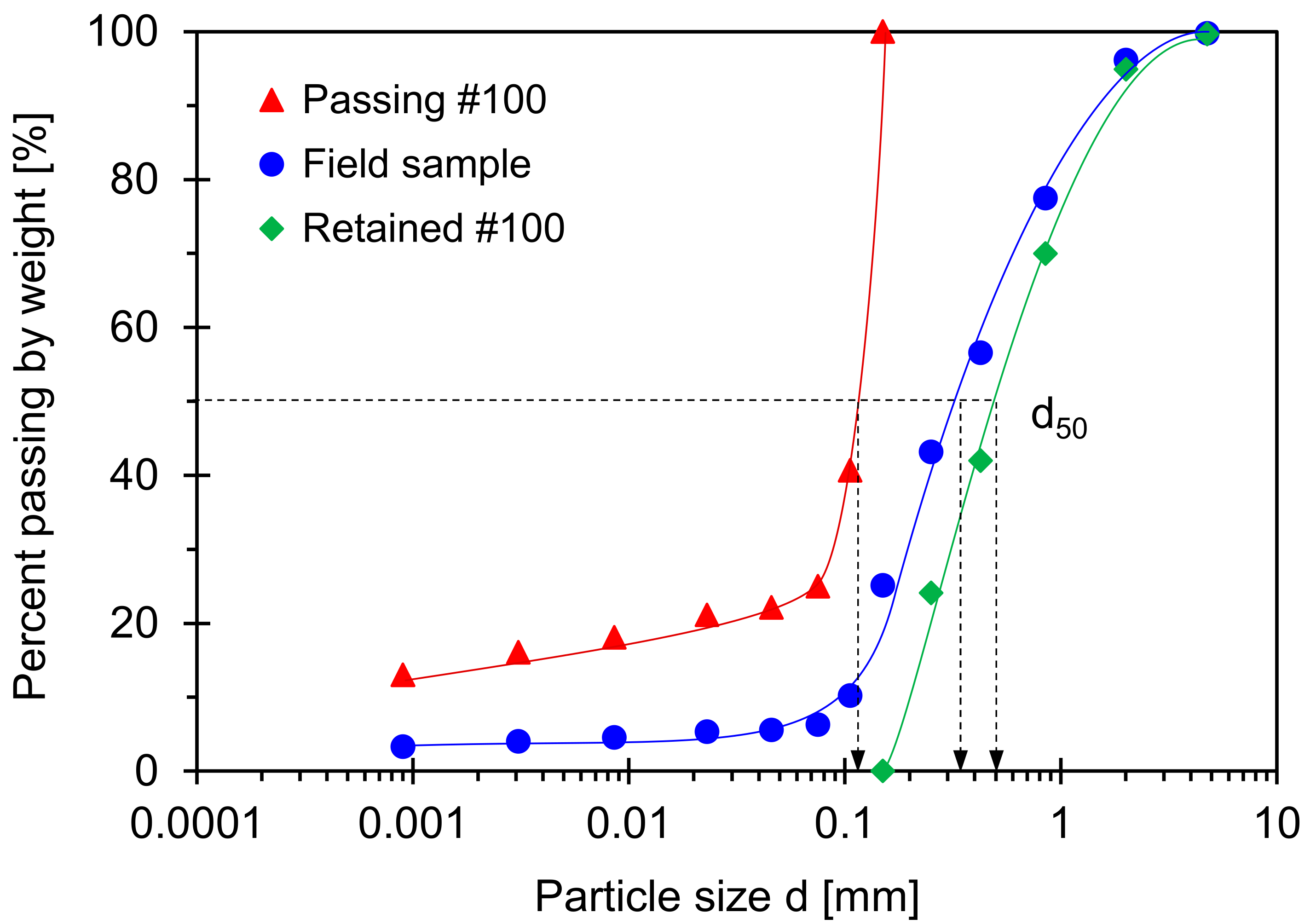
| HPC-1 (19.2~19.35 m) | D10 [mm] | D60 [mm] | D50 [mm] | Cu | Specific Surface Ss [m2/g] | Liquid Limit LL | R | PI | USCS | RSCS |
|---|---|---|---|---|---|---|---|---|---|---|
| Original Field sample | 0.1 | 0.48 | 0.35 | 4.8 | 73.4 | 60.1 | 0.53 | 18.1 | SP-SC | CF |
| Passing through Sieve No. 100 | <0.001 | 0.12 | 0.12 | - | - | - | - | - | - | - |
| Retained on Sieve No. 100 | 0.19 | 0.68 | 0.56 | 3.6 | - | - | - | - | - | - |
Publisher’s Note: MDPI stays neutral with regard to jurisdictional claims in published maps and institutional affiliations. |
© 2021 by the authors. Licensee MDPI, Basel, Switzerland. This article is an open access article distributed under the terms and conditions of the Creative Commons Attribution (CC BY) license (https://creativecommons.org/licenses/by/4.0/).
Share and Cite
Kim, S.Y.; Lee, J.-S.; Park, J. Response of Transitional Mixtures Retaining Memory of In-Situ Overburden Pressure Monitored Using Electromagnetic and Piezo Crystal Sensors. Sensors 2021, 21, 2570. https://doi.org/10.3390/s21072570
Kim SY, Lee J-S, Park J. Response of Transitional Mixtures Retaining Memory of In-Situ Overburden Pressure Monitored Using Electromagnetic and Piezo Crystal Sensors. Sensors. 2021; 21(7):2570. https://doi.org/10.3390/s21072570
Chicago/Turabian StyleKim, Sang Yeob, Jong-Sub Lee, and Junghee Park. 2021. "Response of Transitional Mixtures Retaining Memory of In-Situ Overburden Pressure Monitored Using Electromagnetic and Piezo Crystal Sensors" Sensors 21, no. 7: 2570. https://doi.org/10.3390/s21072570
APA StyleKim, S. Y., Lee, J.-S., & Park, J. (2021). Response of Transitional Mixtures Retaining Memory of In-Situ Overburden Pressure Monitored Using Electromagnetic and Piezo Crystal Sensors. Sensors, 21(7), 2570. https://doi.org/10.3390/s21072570