
Indirect Temperature Measurement in High Frequency Heating Systems


Abstract
:1. Introduction
- High thermal inertia (lag) of the hotend assembly (nozzle+heating block) does not allow rapid temperature regulation of the nozzle during printing;
- Design features of the conventional extruder and drawbacks of the described temperature control methods do not allow the provision of fast and precise temperature control of the extruded material;
- rapid heating of the nozzle due to its isolation from the high power induction heater (peak power > 300 W);
- rapid cooling of the nozzle due to its low mass;
- uniform heating of the nozzle and extruded material due to optimization of the induction heating frequency and geometric shape of the inductor.
2. Materials and Methods
2.1. Temperature Measurement Technique for the Ferromagnetic Nozzle
2.2. Testbed System
2.3. Basics of an Indirect (Eddy-Current) Temperature Measurement Method
3. Results and Discussion
3.1. Desired Signal Amplitude Measurement
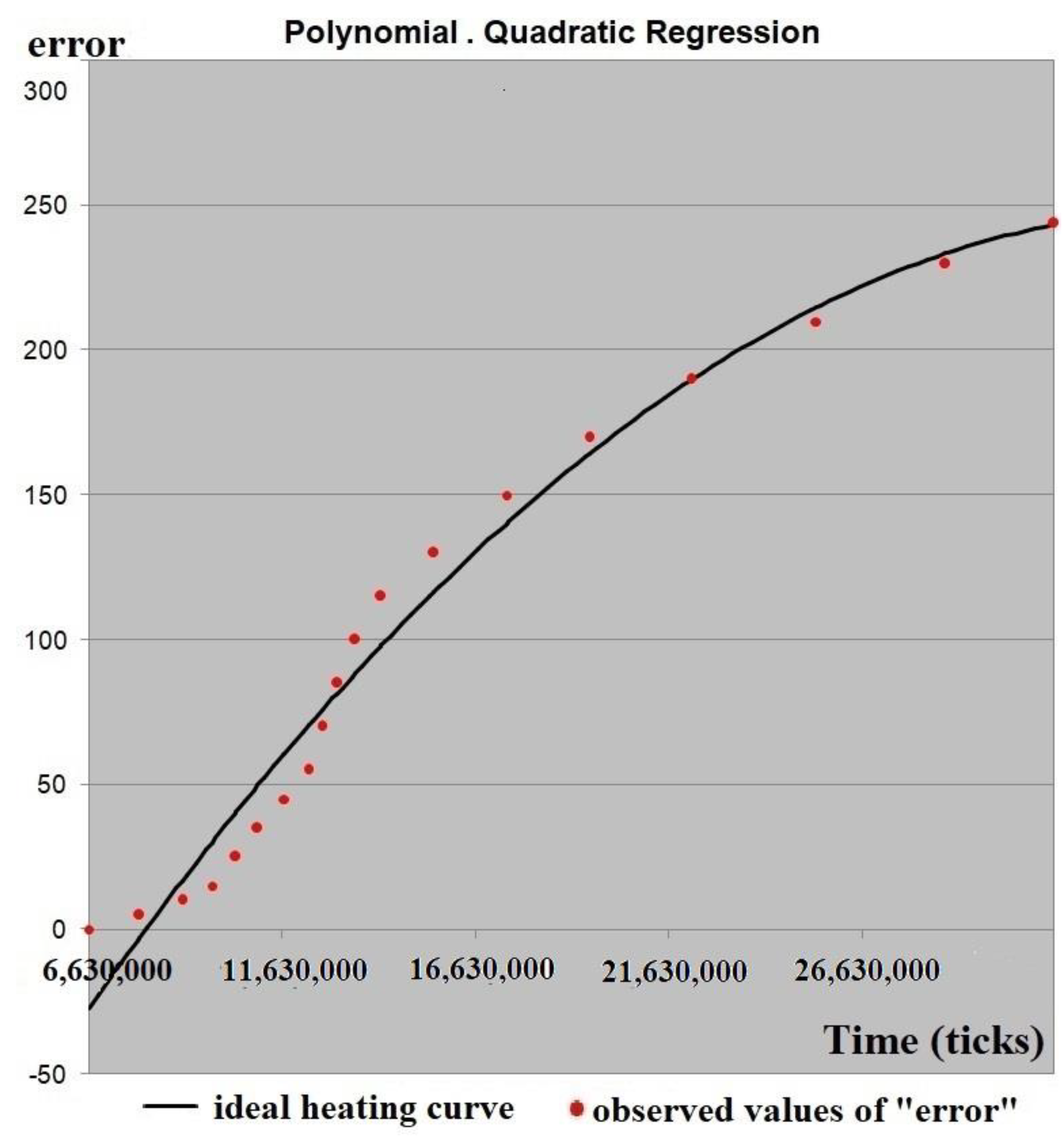
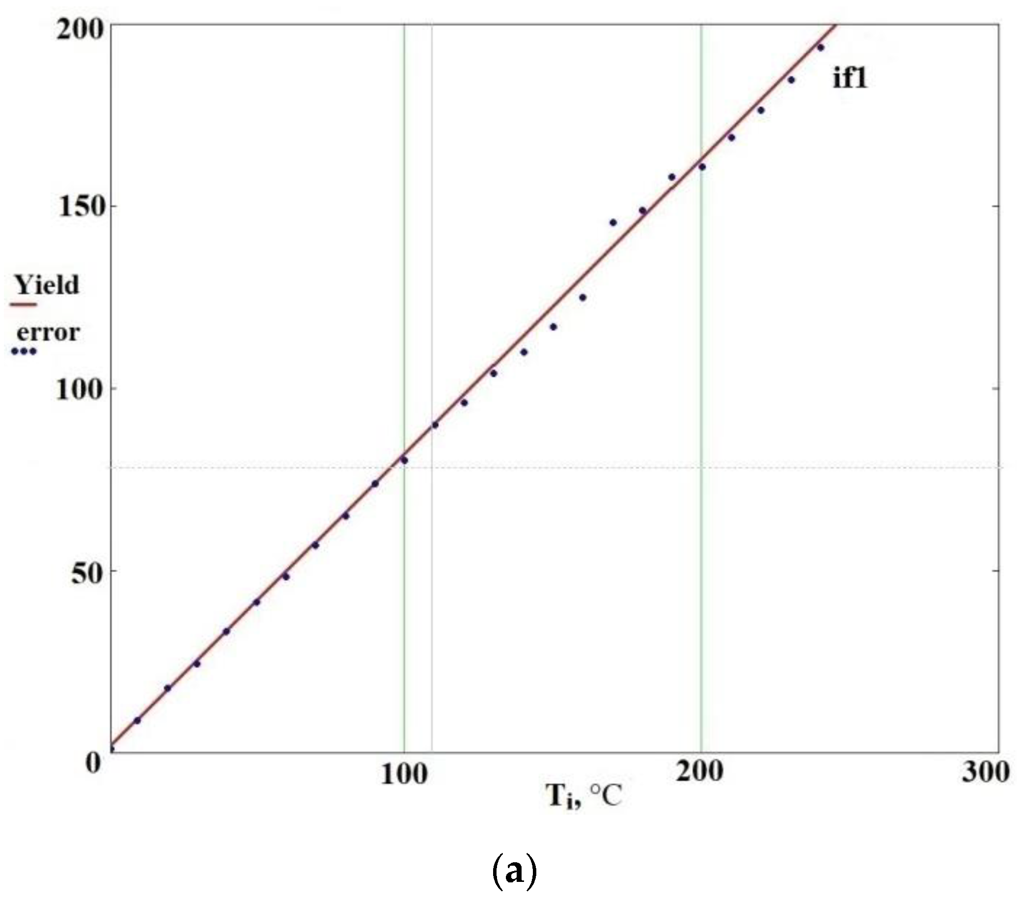
3.2. Regression Model
3.3. Experimental Verification of Proposed Method
- There is no need for additional temperature sensors. The method is based on the analysis of the corresponding resonant circuit parameters;
- It is a non-contact method of measuring temperature;
- There is fast measurement due to a lack of inertial components and thermal contact conduction between the induction heating coil and the nozzle.
4. Conclusions
Author Contributions
Funding
Institutional Review Board Statement
Informed Consent Statement
Data Availability Statement
Conflicts of Interest
References
- Srinivasulu Reddy, K.; Dufera, S. Additive manufacturing technologies. Int. J. Manag. Inf. Technol. Eng. 2016, 4, 89–112. [Google Scholar]
- Sheoran, A.J.; Kumar, H. Fused Deposition modeling process parameters optimization and effect on mechanical properties and part quality: Review and reflection on present research. Mater. Today Proc. 2020, 21, 1659–1672. [Google Scholar]
- Fotovvati, B.; Balasubramanian, M.; Asadi, E. Modeling and Optimization Approaches of Laser-Based Powder-Bed Fusion Process for Ti-6Al-4V Alloy. Coatings 2020, 10, 1104. [Google Scholar] [CrossRef]
- Galati, M.; Di Mauro, O.; Iuliano, L. Finite element simulation of multilayer electron beam melting for the improvement of build quality. Crystals 2020, 10, 532. [Google Scholar] [CrossRef]
- Schröder, M.; Falk, B.; Schmitt, R. Evaluation of Cost Structures of Additive Manufacturing Processes Using a New Business Model. Procedia Cirp 2015, 30, 311–316. [Google Scholar] [CrossRef] [Green Version]
- Abdulhameed, O.; Al-Ahmari, A.; Ameen, W.; Mian, S.H. Additive Manufacturing: Challenges, Trends, and Applications. Adv. Mech. Eng. 2019, 11, 1–27. [Google Scholar] [CrossRef] [Green Version]
- Isasi-Sanchez, L.; Jesus Morcillo-Bellido, J.; Ortiz-Gonzalez, J.I.; Duran-Heras, A. Synergic Sustainability Implications of Additive Manufacturing in Automotive Spare Parts: A Case Analysis. Sustainability 2020, 12, 8461. [Google Scholar] [CrossRef]
- Borschev, Y.P.; Ananiev, A.I.; Kamyshanov, I.V.; Telelyaev, E.N. Application of 3D printing method in manufacture of elements of spacecraft antenna-feeder systems. Eng. J. Sci. Innov. 2020, 9, 1–14. [Google Scholar]
- Latecoere, Accelerates Design Validation and Tool Production with Stratasys Additive Manufacturing. Available online: https://investors.stratasys.com/news-events/press-releases/detail/439/french-aerospace-manufacturer-latcore-accelerates (accessed on 12 December 2020).
- General Electric. Available online: https://www.ge.com/additive/additive-manufacturing/industries/aviation-aerospace (accessed on 16 December 2020).
- Berman, B. 3-D Printing: The New Industrial Revolution. Bus. Horiz. 2012, 55, 155–162. [Google Scholar] [CrossRef]
- Thompson, M.K.; Moroni, G.; Vaneker, T.; Fadel, G.; Campbell, R.I.; Gibson, I.; Bernard, A.; Schulz, J.; Graf, P.; Ahuja, B.; et al. Design for Additive Manufacturing: Trends, Opportunities, Considerations, and Constraints. Cirp Ann. Manuf. Technol. 2016, 65, 737–760. [Google Scholar] [CrossRef] [Green Version]
- Kruth, J.P.; Leu, M.C.; Nakagawa, T. Progress in Additive Manufacturing and Rapid Prototyping. Cirp Ann. 1998, 47, 525–532. [Google Scholar] [CrossRef]
- Boeing. Available online: https://www.boeing.com/features/2013/09/bds-phantom-swift-09-11-13.page (accessed on 22 December 2020).
- Airbus. Available online: https://www.airbus.com/newsroom/news/en/2018/04/bridging-the-gap-with-3d-printing.html (accessed on 10. December 2020).
- Merulla, A.; Gatto, A.; Bassoli, E.; Munteanu, S.I.; Gheorghiu, B.; Pop, M.A.; Bedo, T.; Munteanu, D. Weight reduction by topology optimization of an engine subframe mount, designed for additive manufacturing production. Mater. Today Proc. 2019, 19, 1014–1018. [Google Scholar] [CrossRef]
- Wang, J.Y.; Sama, S.R.; Lynch, P.C.; Manogharan, G. Design and topology optimization of 3D-printed wax patterns for rapid investment casting. Procedia Manuf. 2019, 34, 683–694. [Google Scholar] [CrossRef]
- Javaid, M.; Haleem, A. Additive manufacturing applications in medical cases: A literature based review. Alex. J. Med. 2017, 54, 411–422. [Google Scholar] [CrossRef] [Green Version]
- Haleem, A.; Javaid, M.; Saxena, A. Additive manufacturing applications in cardiology: A review. Egypt. Heart J. 2018, 70, 433–441. [Google Scholar] [CrossRef] [PubMed]
- Sarker, A.; Leary, M.; Fox, K. Metallic additive manufacturing for bone-interfacing implants. Biointerphases 2020, 15, 050801. [Google Scholar] [CrossRef] [PubMed]
- Tiwary, V.K.; Arunkumar, P.; Deshpande, A.S.; Nikhil, P. Surface enhancement of FDM patterns to be used in rapid investment casting for making medical implants. Rapid. Prototyp. J. 2019, 25, 904–914. [Google Scholar] [CrossRef]
- Lee, N. The Lancet Technology: 3D printing for instruments, models, and organs? Lancet 2016, 388, 1368. [Google Scholar] [CrossRef]
- Lupuleasa, D.; Drăgănescu, D.; Hîncu, L.; Tudosă, C.P.; Cioacă, D. Biocompatible polymers for 3D printing. Farmacia 2018, 66, 737–746. [Google Scholar] [CrossRef]
- Arif, U.; Haider, S.; Haider, A.; Khan, N.; Alghyamah, A.A.; Jamila, N.; Khan, M.I.; Almasry, W.A.; Kang, I.K. Biocompatible polymers and their potential biomedical applications: A review. Curr. Pharm. Des. 2019, 25, 3608–3619. [Google Scholar] [CrossRef] [PubMed]
- Honigmann, P.; Sharma, N.; Okolo, B.; Popp, U.; Msallem, B.; Thieringer, F.M. Patient-specific surgical implants made of 3D printed PEEK: Material, technology, and scope of surgical application. BioMed Res. Int. 2018. [Google Scholar] [CrossRef] [Green Version]
- Vaezi, M.; Yang, S. Extrusion-based additive manufacturing of PEEK for biomedical applications. Virtual Phys. Prototyp. 2015, 10, 1–13. [Google Scholar] [CrossRef]
- Ma, R.; Tang, T. Current strategies to improve the bioactivity of PEEK. Int. J. Mol. Sci. 2014, 15, 5426–5445. [Google Scholar] [CrossRef] [Green Version]
- Najeeb, S.; Khurshid, Z.; Matinlinna, J.P.; Siddiqui, F.; Nassani, M.Z.; Baroudi, K. Nanomodified Peek Dental Implants: Bioactive Composites and Surface Modification—A Review. Int. J. Dent. 2015, 2015, 381759. [Google Scholar] [CrossRef] [PubMed] [Green Version]
- Haleem, A.; Javaid, M. Polyether ether ketone (PEEK) and its manufacturing of customised 3D printed dentistry parts using additive manufacturing. Clin. Epidemiol. Glob. Health 2019, 7, 654–660. [Google Scholar] [CrossRef] [Green Version]
- Zhao, C.Y.; Zhao, K.; Li, Y.-C.; Chen, F. Mechanical characterization of biocompatible PEEK by FDM. J. Manuf. Process. Part A 2020, 56, 28–42. [Google Scholar] [CrossRef]
- Panayotov, I.V.; Orti, V.; Cuisinier, F.; Yachouh, J. Polyetheretherketone (PEEK) for medical applications. J. Mater. Sci. Mater. Med. 2016, 27, 118. [Google Scholar] [CrossRef] [PubMed]
- Wang, Y.; Müller, W.-D.; Rumjahn, A.; Schwitalla, A. Parameters influencing the outcome of additive manufacturing of tiny medical devices based on PEEK. Materials 2020, 13, 466. [Google Scholar] [CrossRef] [Green Version]
- Attoye, S.O. A study of fused deposition modeling (FDM) 3-D printing using mechanical testing and thermography. Ph.D. Thesis, Purdue University Graduate School, Pune, India, 2018; pp. 1–129. [Google Scholar]
- Statista. Available online: https://www.statista.com/statistics/560304/worldwide-survey-3d-printing-top-technologies/ (accessed on 24 December 2020).
- Daminabo, S.C.; Goel, S.; Grammatikos, S.A.; Nezhad, H.Y.; Thakur, V.K. Fused Deposition Modeling-Based Additive Manufacturing (3D Printing): Techniques for Polymer Material Systems. Mater. Today Chem. 2020, 16, 100248. [Google Scholar] [CrossRef]
- Chennakesava, P.; Narayan, Y.S. Fused deposition modeling-insights. In Proceedings of the International Conference on Advances in Design and Manufacturing (ICAD&M’14), Tamil Nadu, India, 5–7 December 2014; pp. 1345–1350. [Google Scholar]
- Mortimer, S.; Rowley, J.; Lamb, D. Nozzle. U.S. Patent D762,752, 2 August 2016. [Google Scholar]
- Grimm, T.; Grimm, T.A.; Sociates, Inc. Fused deposition modelling: A technology evaluation. Time-Compress. Technol. 2003, 11, 1–6. [Google Scholar]
- Hofstaetter, T.; Pimentel, R.; Pedersen, D.B.; Mischkot, M. Simulation of a downsized fdm nozzle. In Proceedings of the COMSOL Conference, Pune, India, 27 March 2015. [Google Scholar]
- El Alaiji, R.; Sallaou, M.; Bouayad, A.; Lasri, L. Finite Element Modeling of an Optimized Liquefier Design for 3D Printing of CFRTPCs by Thermal Simulation. In Proceedings of the Advanced Intelligent Systems for Sustainable Development (AI2SD’2019), Marrakech, Morocco, 8–11 July 2019; pp. 337–346. [Google Scholar]
- Jerez-Mesa, R.; Travieso-Rodriguez, J.A.; Corbella, X.; Busqué, R.; Gomez-Gras, G. Finite element analysis of the thermal behavior of a RepRap 3D printer liquefier. Mechatronics 2016, 36, 119–126. [Google Scholar] [CrossRef] [Green Version]
- Lee, C.-W.; Kim, H.-W.; Yu, J.-H.; Park, K. Thermal-Fluid Coupled Analysis of the Nozzle Part for the FDM 3D Printers Considering Flow Characteristics of Cooling Fan. J. Korean Soc. Precis. Eng. 2018, 35, 479–484. [Google Scholar] [CrossRef]
- Chen, Y.; Shi, T.; Lu, L.; Yue, X.; Zhang, J. Optimization design of color mixing nozzle based on multi physical field coupling. In Proceedings of the IOP Conference Series: Earth and Environmental Science, Malang City, Indonesia, 12–13 March 2019; Volome 233. [Google Scholar]
- Sukindar, N.A.; MohdAriffin, M.K.A.; TuahBaharudin, B.T.H.; Binti Jaafar, C.N.A.; Ismail, M.I.S. Analysis on temperature setting for extruding polylactic acid using open source 3D printer. Arpn J. Eng. Appl. Sci. 2017, 12, 1348–1353. [Google Scholar]
- White, D.R.; Hutt, L.; del Campo, C.D.; Izquierdo, C.G. Guide on Secondary Thermometry. Thermistor Thermometry; Bureau International des Poids et Mesures: Sèvres, France, 2014; pp. 1–19. [Google Scholar]
- Pollard, D.; Ward, C.; Herrmann, G.; Etches, J. Filament temperature dynamics in fused deposition modelling and outlook for control. Procedia Manuf. 2017, 11, 536–544. [Google Scholar] [CrossRef]
- Anderegg, D.A.; Bryant, H.A.; Ruffin, D.C.; Skrip, S.M.; Fallon, J.J.; Gilmer, E.L.; Bortner, M.J. In-situ monitoring of polymer flow temperature and pressure in extrusion based additive manufacturing. Addit. Manuf. 2019, 26, 76–83. [Google Scholar] [CrossRef]
- Kuznetsov, V.E.; Solonin, A.N.; Tavitov, A.G.; Urzhumtsev, O.D.; Vakulik, A.H. Increasing of Strength of FDM (FFF) 3D Printed Parts by Influencing on Temperature-Related Parameters of the Process. Rapid Prototyp. J. 2018. [Google Scholar] [CrossRef]
- Ding, S.; Zou, B.; Wang, P.; Ding, H. Effects of nozzle temperature and building orientation on mechanical properties and microstructure of PEEK and PEI printed by 3D-FDM. Polym. Test. 2019, 78, 105948. [Google Scholar] [CrossRef]
- Yang, T.-C. Effect of extrusion temperature on the physico-mechanical properties of unidirectional wood fiber-reinforced polylactic acid composite (WFRPC) components using fused deposition modeling. Polymers 2018, 10, 976. [Google Scholar] [CrossRef] [Green Version]
- Bryan, D.; Peng, F.; Weinheimer, E.; Cakmak, M. FDM from a Polymer Processing Perspective: Challenges and Opportunities. Department of Polymer Engineering University of Akron. Available online: https://www.nist.gov/system/files/documents/mml/Session-4_2-Vogt.pdf (accessed on 2 April 2021).
- Sun, Q.; Rizvi, G.M.; Bellehumeur, C.T.; Gu, P. Effect of processing conditions on the bonding quality of FDM polymer filaments. Rapid Prototyp. J. 2008, 14, 72–80. [Google Scholar] [CrossRef]
- Li, H.; Wang, T.; Sun, J.; Yu, Z. The effect of process parameters in fused deposition modeling on bonding degree and mechanical properties. Rapid Prototyp. J. 2018, 24, 80–92. [Google Scholar] [CrossRef]
- Kuznetsov, V.E.; Solonin, A.N.; Urzhumtsev, O.D.; Schilling, R. Hardware Factors Influencing Strength of Parts Obtained by Fused Filament Fabrication. Polymers 2019, 11, 1870. [Google Scholar]
- Hu, B.; Duan, X.; Xing, Z.; Xu, Z.; Du, C.; Zhou, H.; Chen, R.; Shan, B. Improved design of fused deposition modeling equipment for 3D printing of high-performance PEEK parts. Mech. Mater. 2019, 137, 103139. [Google Scholar] [CrossRef]
- Fedulov, A.A.; Saonov, M.M.; Kantor, S.V.; Lomov, P. Modeling of thermoplastic composites solidification and estimation of residual stresses. Compos. Nanostruct. 2017, 9, 102–122. [Google Scholar]
- Wang, P.; Zou, B.; Xiao, H.; Ding, S.; Huang, C. Effects of printing parameters of fused deposition modeling on mechanical properties, surface quality, and microstructure of PEEK. J. Mater. Process. Technol. 2019, 271, 62–74. [Google Scholar] [CrossRef]
- Deng, X.; Zeng, Z.; Peng, B.; Yan, S.; Ke, W. Mechanical properties optimization of poly-ether-ether-ketone via fused deposition modeling. Materials 2018, 11, 216. [Google Scholar] [CrossRef] [Green Version]
- Geng, P.; Zhao, J.; Wu, W.; Ye, W.; Wang, Y.; Wang, S.; Zhang, S. Effects of extrusion speed and printing speed on the 3D printing stability of extruded PEEK filament. J. Manuf. Proc. 2019, 37, 266–273. [Google Scholar] [CrossRef]
- Gardner, J.M.; Stelter, C.J.; Yashin, E.A.; Siochi, E.J. High Temperature Thermoplastic Additive Manufacturing Using Low-Cost, Open-Source Hardware; National Aeronautics and Space Administration, Langley Research Center: Hampton, VA, USA, 2016. [Google Scholar]
- Ning, F.; Cong, W.; Hu, Y.; Wang, H. Additive manufacturing of carbon fiber-reinforced plastic composites using fused deposition modeling: Effects of process parameters on tensile properties. J. Compos. Mater. 2017, 51, 451–462. [Google Scholar] [CrossRef]
- Savushkin, A.V.; Lekomtsev, P.L.; Niyazov, A.M.; Olin, N.L. Electrotechnology (Elektrotekhnologiya), Textbook, Izhevsk; Izhevsk State Agricultural Academy: Izhevsk, Russia, 2013; 45p. [Google Scholar]
- Oskolkov, A.; Trushnikov, D.; Bezukladnikov, I. Application of induction heating in the FDM/FFF 3D manufacturing. J. Phys. Conf. Ser. 2021, 1730, 012005. [Google Scholar] [CrossRef]
- Sebko, V.V. Non-contact complex multi-parameter eddy- current control of samples of weakly ferromagnetic and ferromagnetic liquid media. Electr. Eng. (Elektrotekhnika I Elektromekhanika) 2011, 1, 53–57. [Google Scholar]
- Sebko, V.V. Eddy-current multiparameter method for control of flat products of aviation equipment. Aviat. Space Technol. 2010, 5, 83–90. [Google Scholar]
- Sebko, V.V. Influence of temperature on magnetic permeability and specific electrical resistance of a cylindrical product. Electr. Eng. (Elektrotekhnika I Elektromekhanika) 2003, 3, 44–47. [Google Scholar]
- Franco, C.; Acero, J.; Alonso, R.; Sags, C.; Paesa, D. Inductive sensor for temperature measurement in induction heating applications. IEEE Sens. J. 2012, 12, 996–1003. [Google Scholar] [CrossRef]
- Pinilla, J.M.B.; Duce, I.E.; Jimenez, J.R.G.; Blasco, P.J.H.; Gill, S.L.; Aznar, F.M. Temperature Control for an Inductively Heated Heating Element. U.S. Patent 7,692,121, 6 April 2010. [Google Scholar]
- Smalcerz, A.; Przylucki, R. Impact of electromagnetic field upon temperature measurement of induction heated charges. Int. J. Thermophys. 2013, 34, 667–679. [Google Scholar] [CrossRef] [Green Version]
- Tan, W.S. Application of Induction Heating to 3D Print Low Melting Point Metal Alloy: Final Project Summary Report 2015, UNSW@ADFA; IOP: Bristol, UK, 2015; pp. 1–13. [Google Scholar]
- Bauer, U.; Bandiera, N.G.; Sachs, E.M. Induction Heating Systems and Techniques for Fused Filament Metal Fabrication. U.S. Patent 0,118,252, 25 April 2019. [Google Scholar]
- Pilavdzie, J.I.; Buren, S.V.; Kagan, V.G. Apparatus for Inductive and Resistive Heating of an Object. U.S. Patent 7,041,944, 9 May 2006. [Google Scholar]
- A Kind of Induction, 3D Printer Extruder. CN Patent 105,216,334, 1 June 2016.
- Elserman, M.; Versteegh, J.A.; Zalm, E. Inductive Nozzle Heating Assembly. U.S. Patent 0,094,726, 2017. [Google Scholar]
- Dashkin, A.V.; Karpov, M.B.; Popov, U.D. Printing Head of the Device for Volume Printing with Melted Metal. Patent 170,109, 2017. [Google Scholar]
- Van Pelt, W. Method and Printer Head for 3D Printing of Glass. EU Patent 3,042,751, 2016. [Google Scholar]
- Stirling, R.L.; Chilson, L.; English, A. Inductively Heated Extruder Heater. U.S. Patent 9,596,720, 2017. [Google Scholar]
- Phase-Shifted Full Bridge DC/DC Power Converter Design Guide; Texas Instrumments: Dallas, TX, USA, 2015.
- Seltzer, D.; Zane, R. Feedback control of phase shift modulated half bridge circuits for zero voltage switching assistance. In Proceedings of the 2013 IEEE 14th Workshop on Control and Modeling for Power Electronics (COMPEL), Salt Lake City, UT, USA, 23–26 June 2013; pp. 1–7. [Google Scholar]
- Dieckerhoff, S.; Ruan, M.J.; De Doncker, R.W. Design of an IGBT-based LCL-resonant inverter for high-frequency induction heating. In Proceedings of the Conference Record of the 1999 IEEE Industry Applications Conference, Thirty-Forth IAS Annual Meeting, Phoenix, AZ, USA, 3–7 October 1999; Volume 3, pp. 2039–2045. [Google Scholar]
- Vorokh, D.A.; Makhov, A.I. Resonant converter with pulse-width adjustment of output voltage. Electron. Meas. Equip. Radio Eng. Commun. (Elektron. Izmer. Radiotekhnikaisvyaz’) 2016, 15, 143–155. [Google Scholar]
- MIPT. Magnitnie Svoistva Veshestva; Moscow Institute of Physics and Technology: Moscow, Russia, 2007; 29p. [Google Scholar]
- Adrian, S. Nastase, Design a Bipolar to Unipolar Converter to Drive an ADC. Available online: https://masteringelectronicsdesign.com/design-a-bipolar-to-unipolar-converter/ (accessed on 16 December 2020).
- Improving ADC Resolution by Oversampling and Averaging; Silicon Laboratories Inc.: Austin, TX, USA, 2015.
- AVR121: Enhancing ADC Resolution by Oversampling // Atmel Corporation, 2005. Available online: ww1.microchip.com/downloads/en/appnotes/doc8003.pdf (accessed on 16 December 2020).
- Lam, Y.F. Harry Analog and Digital Filters: Design and Realization; Prentice-Hall: Upper Saddle River, NJ, USA, 1979; 632p. [Google Scholar]
- Ramer-Douglas-Peucker Algorithm. Available online: https://karthaus.nl/rdp/ (accessed on 10 December 2020).
- Wang, J.Y.; Xu, D.D.; Sun, W.; Du, S.M.; Guo, J.J.; Xu, G.J. Effects of nozzle-bed distance on the surface quality and mechanical properties of fused filament fabrication parts. In IOP Conference Series: Materials Science and Engineering; IOP Publishing: London, UK, 2019; Volume 479, p. 12094. [Google Scholar]
- Raju, M.; Gupta, M.K.; Bhanot, N.; Sharma, V.S. A hybrid PSO–BFO evolutionary algorithm for optimization of fused deposition modelling process parameters. J. Intell. Manuf. 2018, 1–16. [Google Scholar] [CrossRef]
- Laeng, J.; Khan, Z.A.; Khu, S. Optimizing flexible behaviour of bow prototype using Taguchi approach. J. Appl. Sci. 2006, 6, 622–630. [Google Scholar] [CrossRef]
- Srivastava, M.; Rathee, S. Optimisation of FDM process parameters by Taguchi method for imparting customised properties to components. Virtual Phys. Prototyp. 2018, 13, 203–210. [Google Scholar] [CrossRef]
- Dong, G.; Wijaya, G.; Tang, Y.; Zhao, Y.F. Optimizing process parameters of fused deposition modeling by Taguchi method for the fabrication of lattice structures. Addit. Manuf. 2018, 19, 62–72. [Google Scholar] [CrossRef] [Green Version]
- Adikari Appuhamillage, G. New 3D Printable Polymeric Materials for Fused Filament Fabrication (FFF). Ph.D. Thesis, The University of Texas at Dallas, Richardson, TX, USA, 2018. [Google Scholar]
- Lee, B.H.; Abdullah, J.; Khan, Z.A. Optimization of rapid prototyping parameters for production of flexible ABS object. J. Mater. Process. Technol. 2005, 169, 54–61. [Google Scholar] [CrossRef]
- Srivastava, M.; Rathee, S.; Maheshwari, S.; Kundra, T. Multi-objective optimization of fused deposition modelling process parameters using RSM and fuzzy logic for build time and support material. Int. J. Rapid Manuf. 2018, 7, 25–42. [Google Scholar] [CrossRef]
- Ahn, S.-H.; Montero, M.; Odell, D.; Roundy, S.; Wright, P.K. Anisotropic material properties of fused deposition modeling ABS. Rapid Prototyp. J. 2002, 8, 248–257. [Google Scholar] [CrossRef] [Green Version]
- Attoye, S.; Malekipour, E.; El-Mounayri, H. Correlation between ProcessParameters and Mechanical Properties in Parts Printed by the FusedDeposition Modeling. Conference Proceedings of the Society for Experimental Mechanics. Mech. Addit. Adv. Manuf. 2019, 8, 35–41. [Google Scholar]
- Torres, J.; Cotelo, J.; Karl, J.; Gordon, A.P. Mechanical property optimization ofFDM PLA in shear with multiple objectives. JOM 2015, 67, 1183–1193. [Google Scholar] [CrossRef]
- Liu, X.; Zhang, M.; Li, S.; Si, L.; Peng, J.; Hu, Y. Mechanical property parametricappraisal of fused deposition modeling parts based on the gray Taguchimethod. Int. J. Adv. Manuf. Technol. 2017, 89, 2387–2397. [Google Scholar] [CrossRef]
- Fernandes, J.; Deus, A.M.; Reis, L.; Vaz, M.F.; Leite, M. Study of the influence of 3Dprinting parameters on the mechanical properties of PLA. In Proceedings of the 3rd International Conference on Progress in Additive Manufacturing (Pro-AM2018), Singapore, 14–17 May 2018. [Google Scholar]
- Cho, E.E.; Hein, H.H.; Lynn, Z.; Hla, S.J.; Tran, T. Investigation on influence of infillpattern and layer thickness on mechanical strength of PLA material in 3Dprinting technology. J. Eng. Sci. Res. 2019, 3, 27–37. [Google Scholar]
- Alafaghania, A.; Qattawi, A.; Alrawi, B.; Guzman, A. Experimental Optimization of Fused Deposition Modelling Processing Parameters: A Design-for-Manufacturing Approach. 45th SME North American Manufacturing Research Conference, NAMRC 45, LA, USA. Procedia Manuf. 2017, 10, 791–803. [Google Scholar] [CrossRef]
- Beniak, J.; Krizˇan, P.; Šooš, L.; Matúš, M. Research on Shape and DimensionalAccuracy of FDM Produced Parts. IOP Conf. Ser. Mater. Sci. Eng. 2019, 501, 012030. [Google Scholar] [CrossRef]
- Guessasma, S.; Belhabib, S.; Nouri, H. Microstructure and mechanical performance of 3D printed wood-PLA/PHA using fused deposition modelling: Effect of printing temperature. Polymers 2019, 11, 1778. [Google Scholar] [CrossRef] [Green Version]
- Benwood, C.; Anstey, A.; Andrzejewski, J.; Misra, M.; Mohanty, A.K. Improving the impact strength and heat resistance of 3D printed models: Structure, property, and processing correlationships during fused deposition modeling (FDM) of poly (lactic acid). Omega 2018, 3, 4400–4411. [Google Scholar] [CrossRef]
- Yang, C.; Tian, X.; Li, D.; Cao, Y.; Zhao, F.; Shi, C. Influence of thermal processing conditions in 3D printing on the crystallinity and mechanical properties of PEEK material. J. Mater. Process. Technol. 2017, 248, 1–7. [Google Scholar] [CrossRef]
- Arif, M.F.; Kumar, S.; Varadarajan, K.M.; Cantwell, W.J. Performance of biocompatible PEEK processed by fused deposition additive manufacturing. Mater. Des. 2018, 146, 249–259. [Google Scholar] [CrossRef]


| Temperature °C | Error | |||
|---|---|---|---|---|
| 0.2% | 10% | 20% | 100% | |
| 110 | 90 | 83 | 75 | 36.5 |
| 120 | 96 | 88 | 80 | 42 |
| 250 | 201.3 | 182.3 | 164 | 74.5 |
| 280 | 224 | 202.5 | 184 | 84 |
| 400 | 320.2 | 290 | 262 | 118 |
| 440 | 353.7 | 320.3 | 289 | 129 |
| 750 | 601.3 | 542.5 | 489 | 215 |
| Coefficient | Estimate | Std Error |
|---|---|---|
| C | 0.797 | 1.18 |
| A | 0.825 | 2.717 × 10⁻³ |
| B | 1.081 × 10⁻⁴ | 1.006 × 10⁻⁴ |
| AB | −7.085 × 10⁻⁶ | 2.315 × 10⁻⁷ |
| BB | 4.951 × 10⁻¹⁰ | 1.982 × 10⁻⁹ |
| ABB | −1.207 × 10⁻¹⁰ | 4.562 × 10⁻¹² |
| Material | Nozzle Temperature °C | Bed Temperature °C | Raster Angle/No. | Extrusion Speed, mm/s | Nozzle Diameter, mm | Layer Thickness, mm | |
|---|---|---|---|---|---|---|---|
| −45°:45° | 0°:90° | ||||||
| Acrylonitrile butadiene styrene (ABS) | 240 | 110 | 1 | 2 | 40 | 0.6 | 0.2 |
| 250 | 3 | 4 | |||||
| Polylactic acid (PLA) | 210 | 60 | 1 | 2 | |||
| 220 | 3 | 4 | |||||
| Material | No. | Tensile Strength, MPa |
|---|---|---|
| ABS | 1 | 43,58 |
| 2 | 39,44 | |
| 3 | 36,71 | |
| 4 | 37,16 | |
| PLA | 1 | 59,61 |
| 2 | 64,47 | |
| 3 | 62,64 | |
| 4 | 60,91 |
| Initial Temperature/Final Temperature °C | Induction Heated (Proposed) Nozzle, Cooling Time, s | Conventional Hotend Assembly (Nozzle + Heating Block), Cooling Time, s |
|---|---|---|
| 300/250 | 5 | 34 |
| 250/230 | 3 | 22 |
| 250/200 | 9 | 60 |
| 200/150 | 13 | 80 |
| 150/100 | 22 | 120 |
| 100/50 | 41 | 250 |
| 250/50 | 82 | 450 |
| Target Temperature, °C | Steady State (After 30 s, Averaged over 5 s), °C | Value Fluctuations (10 Consecutive Measurements after 30 s, in 5 s. Intervals, No Averaging), °C | Setting Time after Disabling Heater, s | Max Overshoot, °C | |
|---|---|---|---|---|---|
| Proposed method | 250 | 248.1 | 247.9–248.2 | 0.3 | 1.3 |
| Thermocouple inside, 10% | 236.3 | 236.2–236.3 | 12.8 | 26 | |
| Thermocouple inside, 50% (reference) | 250.1 | 250.0–250.2 | 6.3 | 11 | |
| Thermocouple inside, 90% | 221.4 | 221.3–221.6 | 18.5 | 38 | |
| Thermocouple on surface, 10% | 235.4 | 235.3–235.5 | 3.2 | 6 | |
| Thermocouple on surface, 50% | 250.0 | 249.9–250.1 | 2.5 | 4 | |
| Thermocouple on surface, 90% | 216.5 | 216.4–216.7 | 4.8 | 8 |
Publisher’s Note: MDPI stays neutral with regard to jurisdictional claims in published maps and institutional affiliations. |
© 2021 by the authors. Licensee MDPI, Basel, Switzerland. This article is an open access article distributed under the terms and conditions of the Creative Commons Attribution (CC BY) license (https://creativecommons.org/licenses/by/4.0/).
Share and Cite
Oskolkov, A.; Bezukladnikov, I.; Trushnikov, D. Indirect Temperature Measurement in High Frequency Heating Systems. Sensors 2021, 21, 2561. https://doi.org/10.3390/s21072561
Oskolkov A, Bezukladnikov I, Trushnikov D. Indirect Temperature Measurement in High Frequency Heating Systems. Sensors. 2021; 21(7):2561. https://doi.org/10.3390/s21072561
Chicago/Turabian StyleOskolkov, Alexander, Igor Bezukladnikov, and Dmitriy Trushnikov. 2021. "Indirect Temperature Measurement in High Frequency Heating Systems" Sensors 21, no. 7: 2561. https://doi.org/10.3390/s21072561
APA StyleOskolkov, A., Bezukladnikov, I., & Trushnikov, D. (2021). Indirect Temperature Measurement in High Frequency Heating Systems. Sensors, 21(7), 2561. https://doi.org/10.3390/s21072561