
An Efficient 3D Human Pose Retrieval and Reconstruction from 2D Image-Based Landmarks


Abstract
1. Introduction
2. Related Work
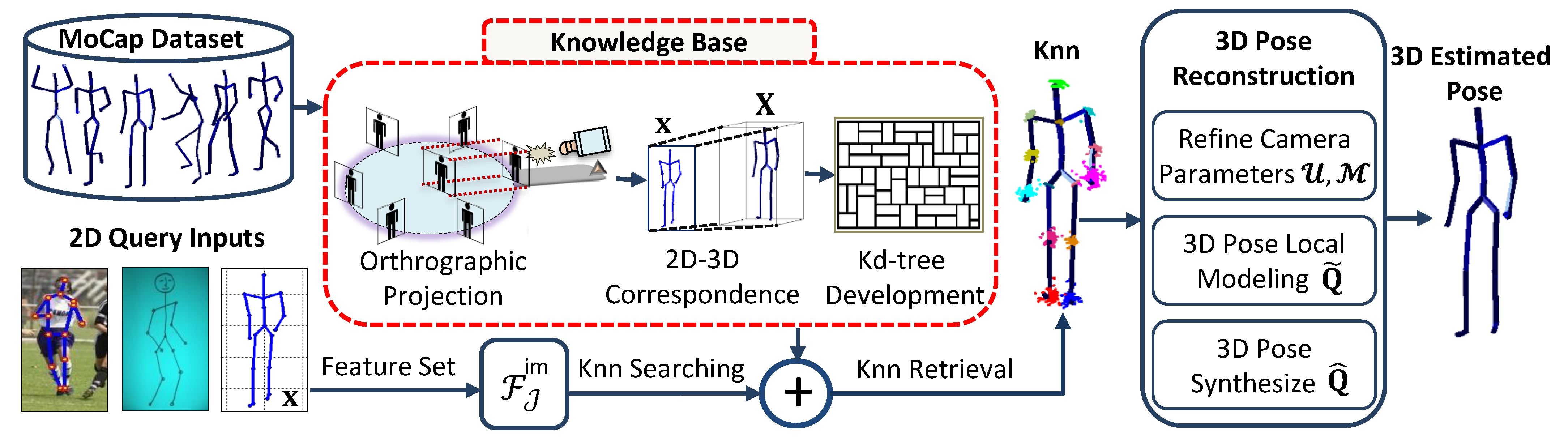
3. Methodology
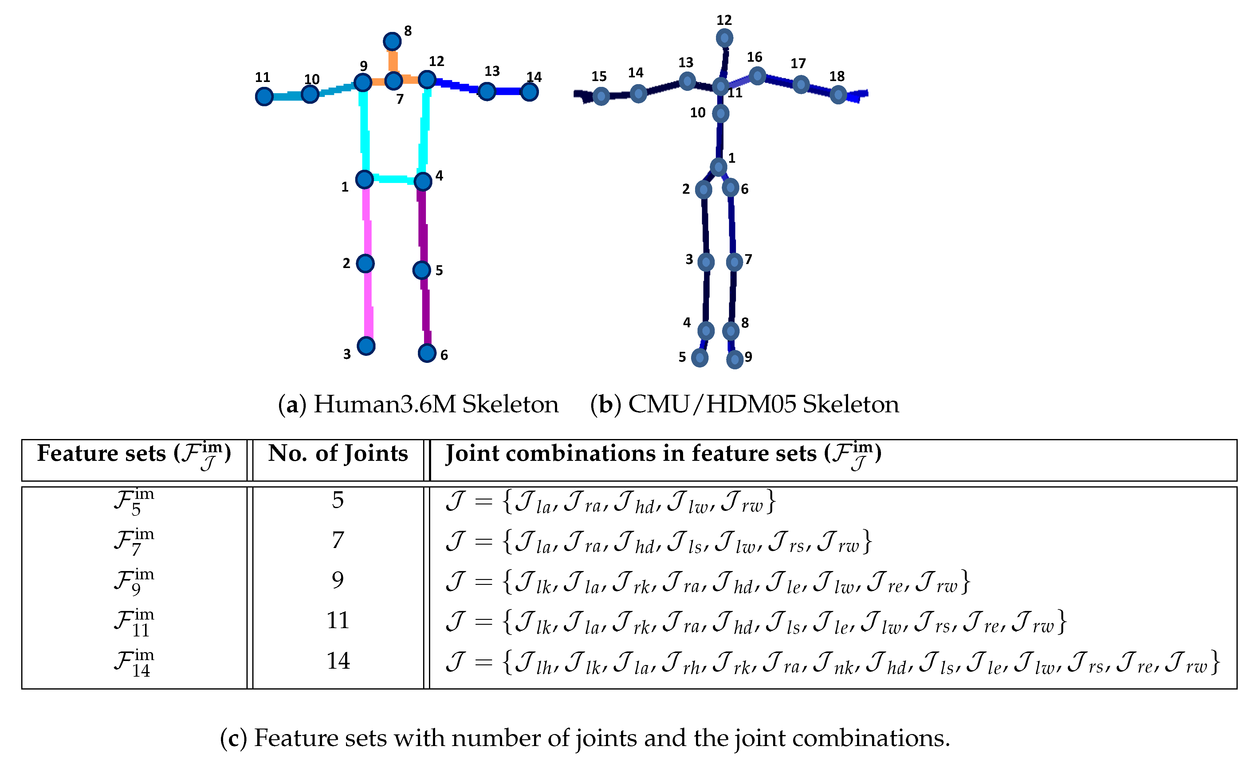
3.1. Pose Skeleton Description
3.2. Normalization
3.2.1. Translational Normalization
3.2.2. Orientational Normalization
3.2.3. Skeleton Size Normalization
3.3. Search and Retrieval
3.4. Camera Parameters
3.5. Pose Reconstruction
3.5.1. Retrieved Pose Error
3.5.2. Projection Control Error
4. Experiments
4.1. Datasets
4.1.1. Mocap Datasets
4.1.2. Input Datasets
Synthetic 2D Dataset
PARSE Dataset
Hand-Drawn Sketches Dataset
4.2. Parameters
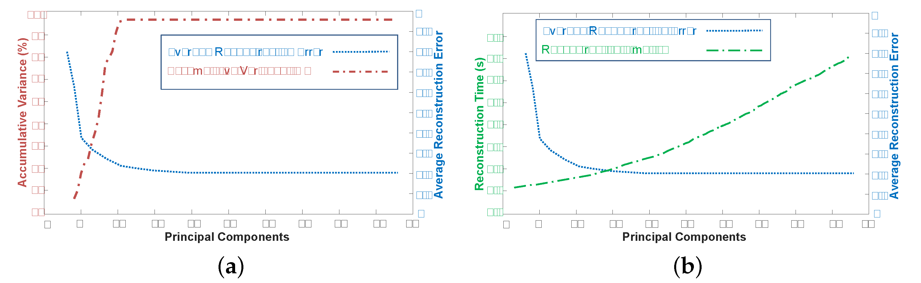
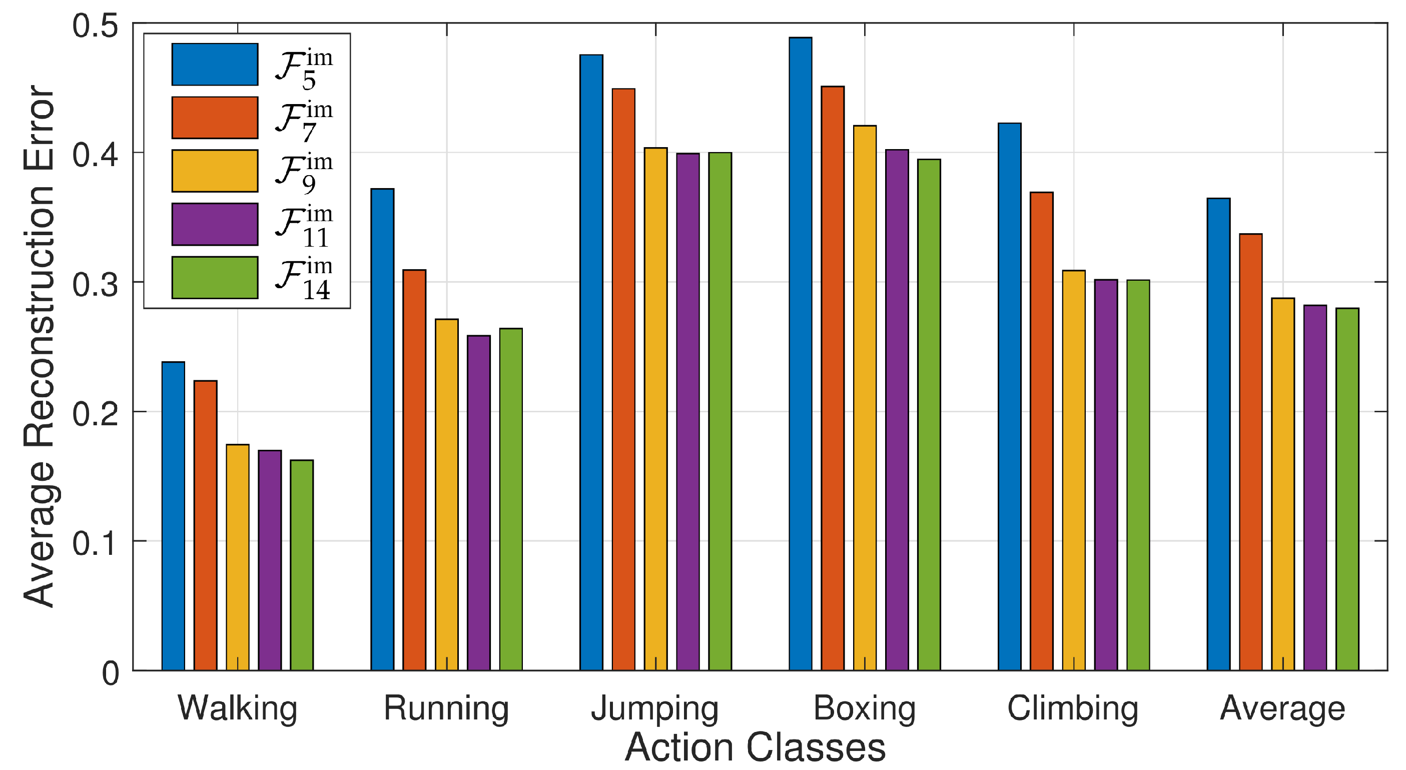
4.2.1. Principal Components
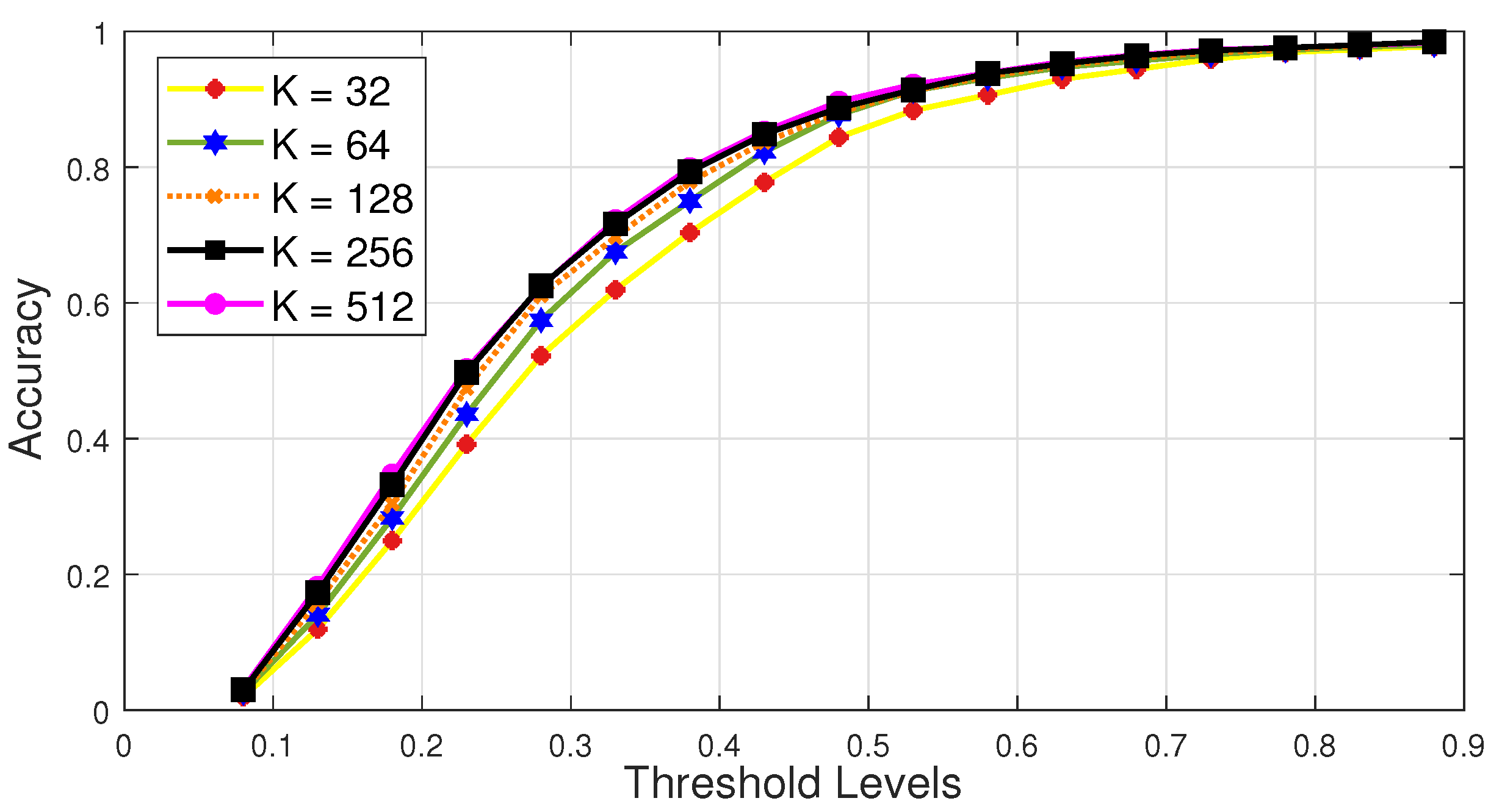
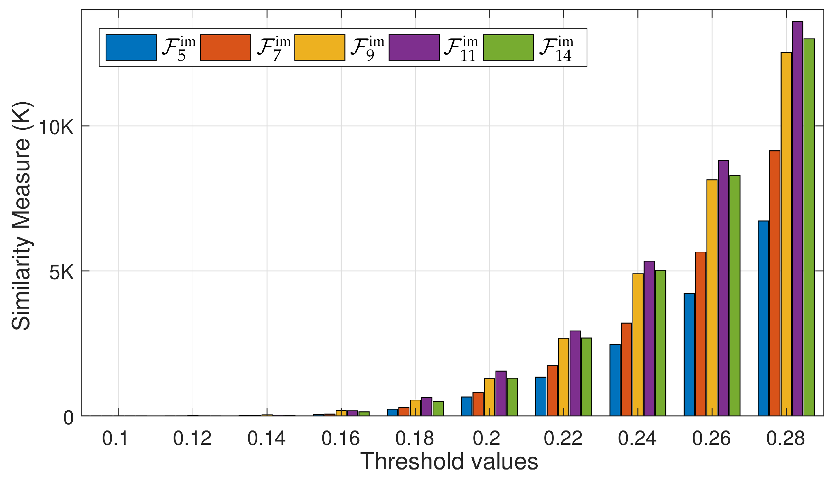
4.2.2. Nearest Neighbors
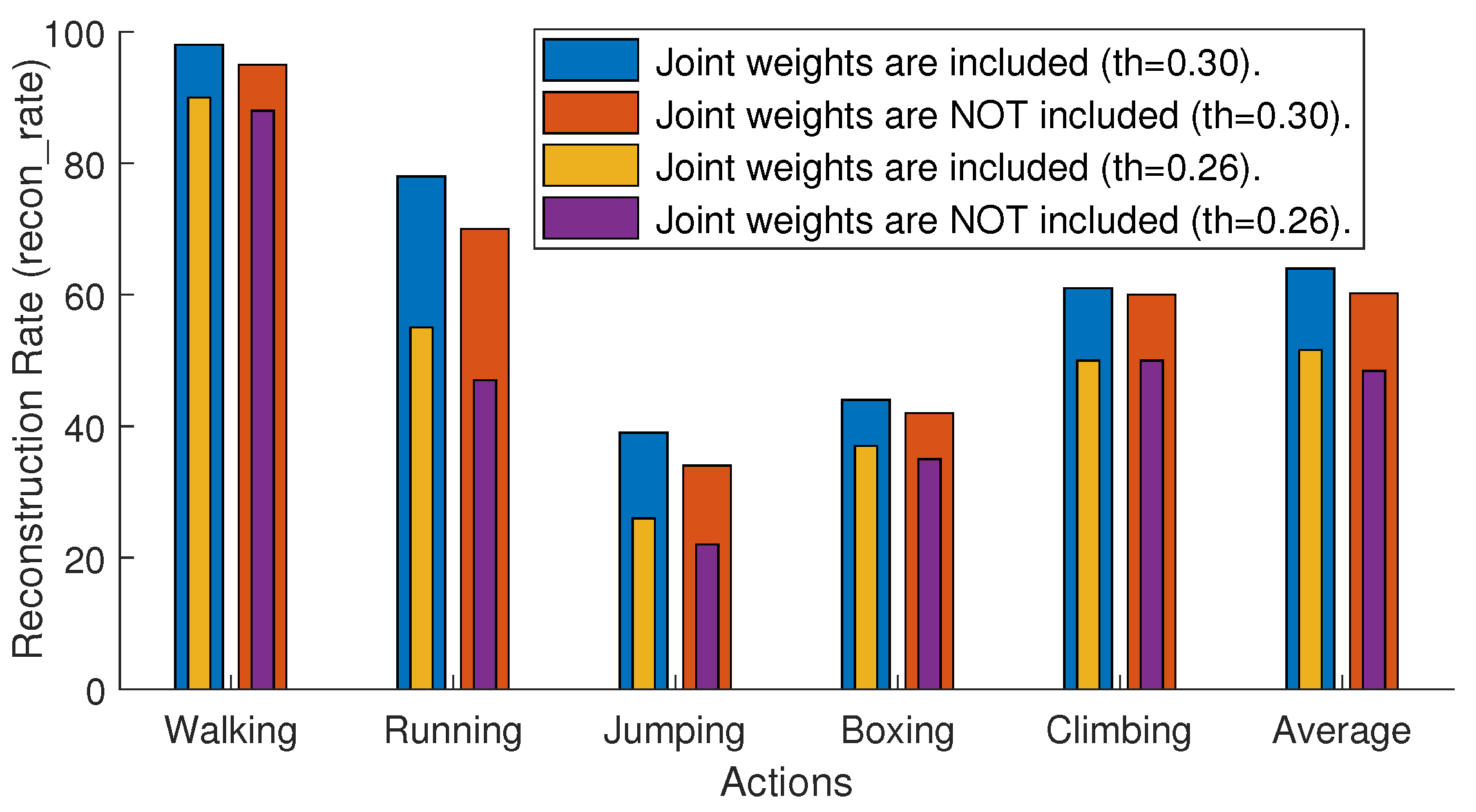
4.2.3. Joint Weights
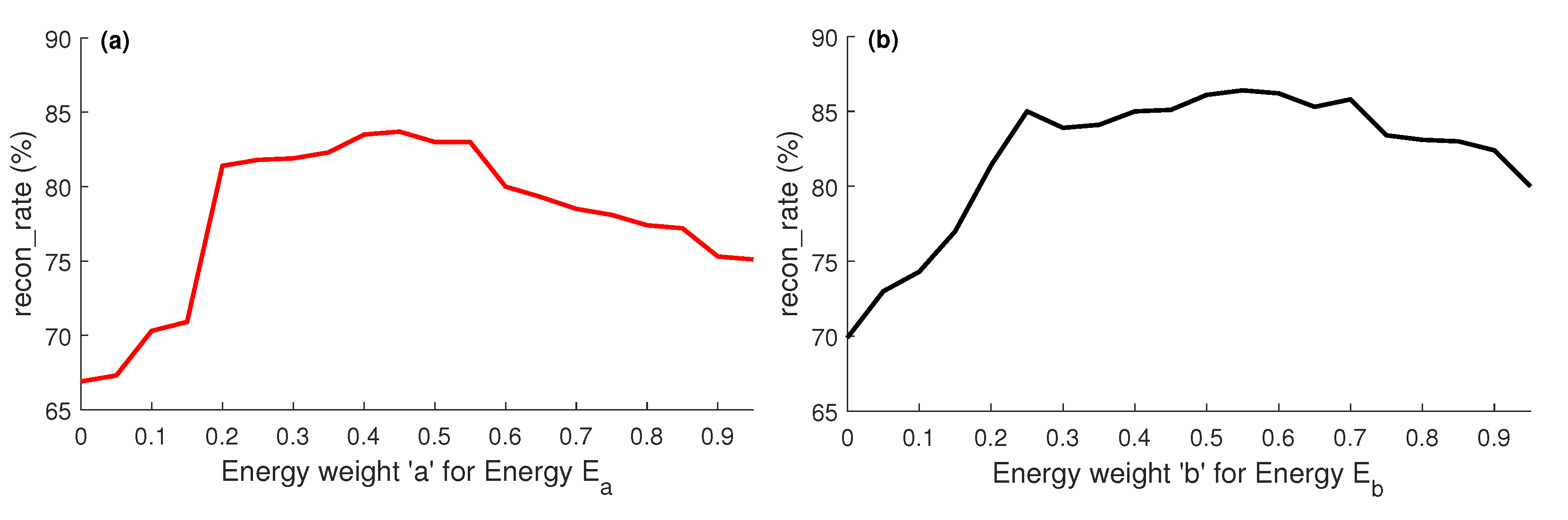
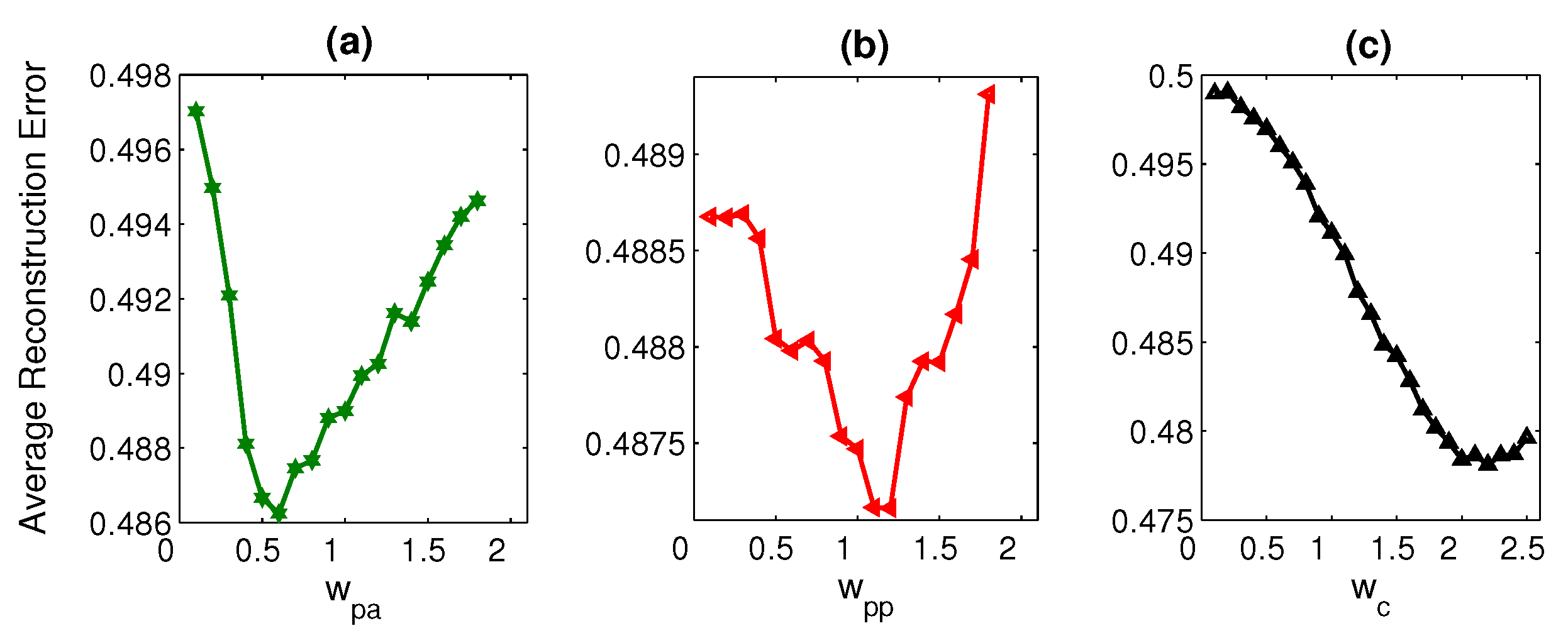
4.2.4. Energy Weights
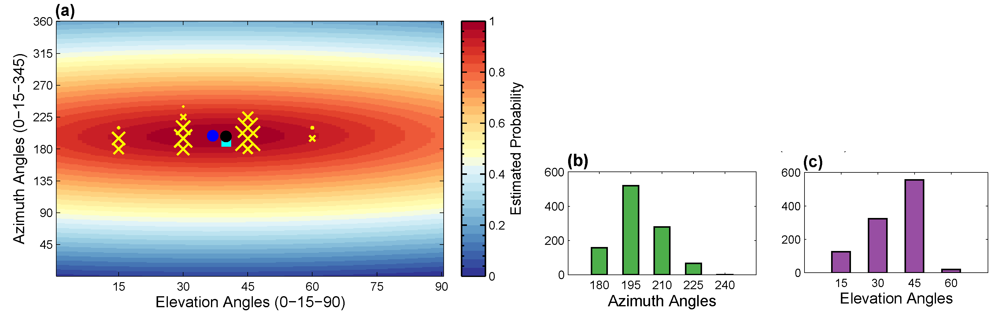
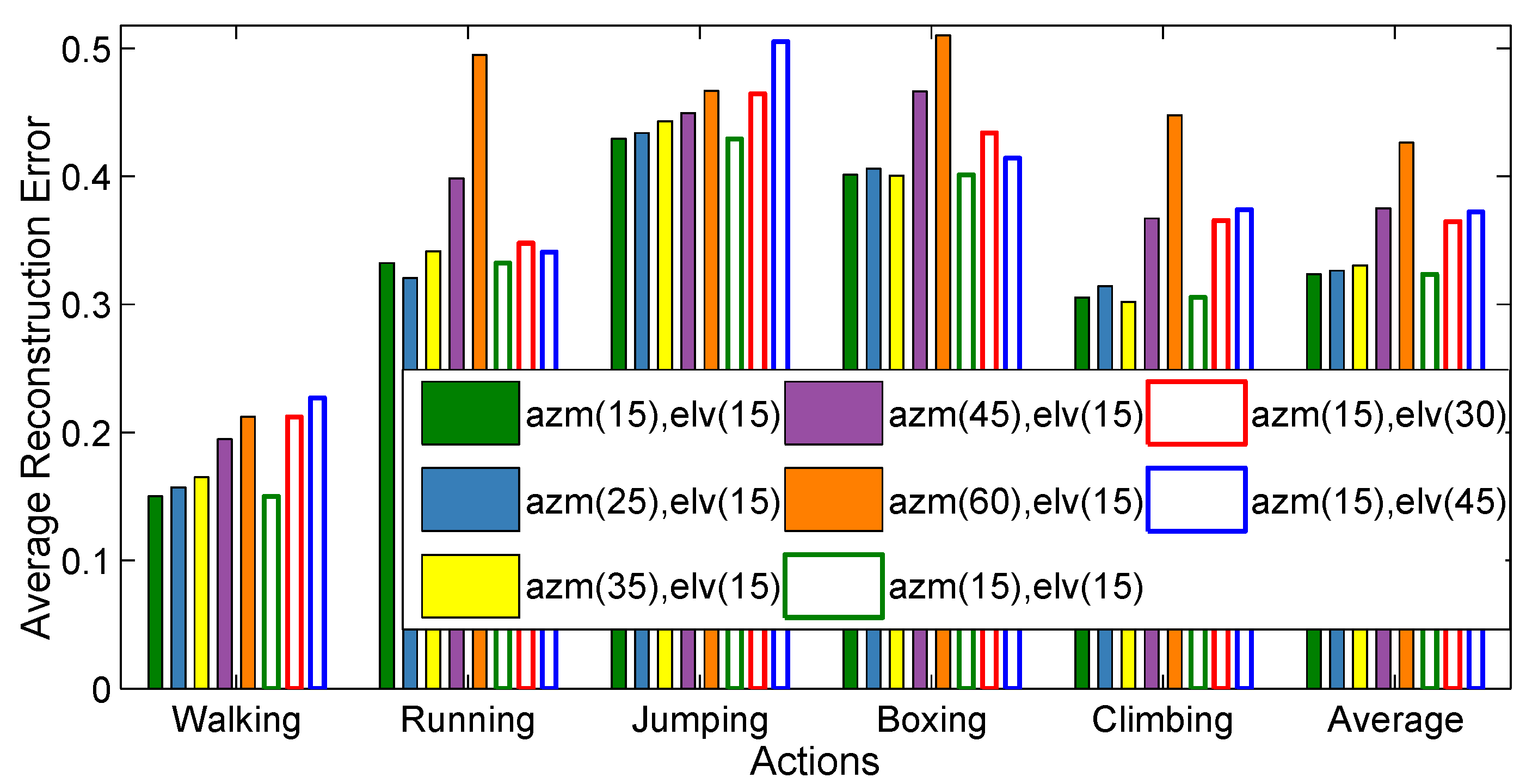
4.2.5. Virtual Cameras
- First, we create virtual cameras just by fixing the elevation (elv) angles (01590) and varying the azimuth (azm) angles (0345 with 15, 25, 35, 45, and 60 step sizes). As a result, we create several virtual cameras as, with azimuth and elevation incremental step sizes , respectively.
- Second, we generate virtual cameras by fixing the azimuth (azm) angles (015345) and by varying the elevation (elv) angles (090 with 15, 30, and 45 step sizes). Consequently, several virtual cameras are created as, with azimuth and elevation incremental step sizes respectively.
4.3. Search and Retrieval
4.4. Quantitative Evaluation
4.4.1. Evaluation on
4.4.2. Evaluation on
4.4.3. Evaluation on
4.4.4. Evaluation on
4.4.5. Evaluation on Noisy Input Data
4.5. Qualitative Evaluation
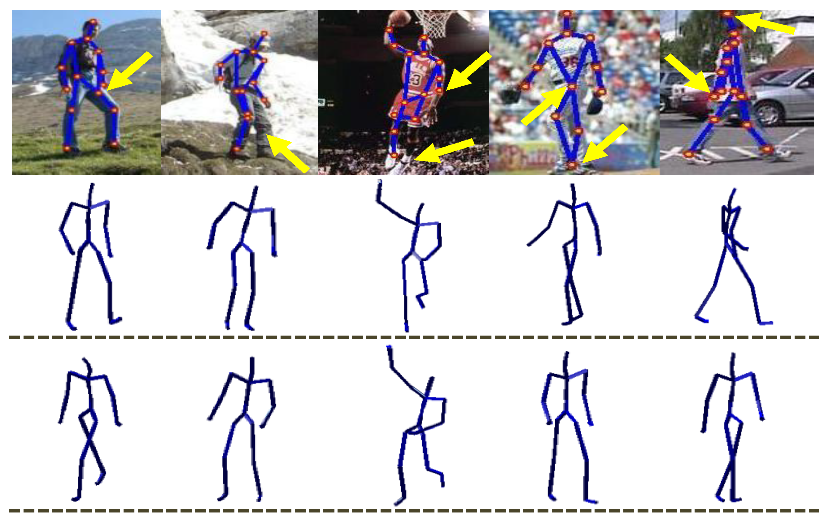
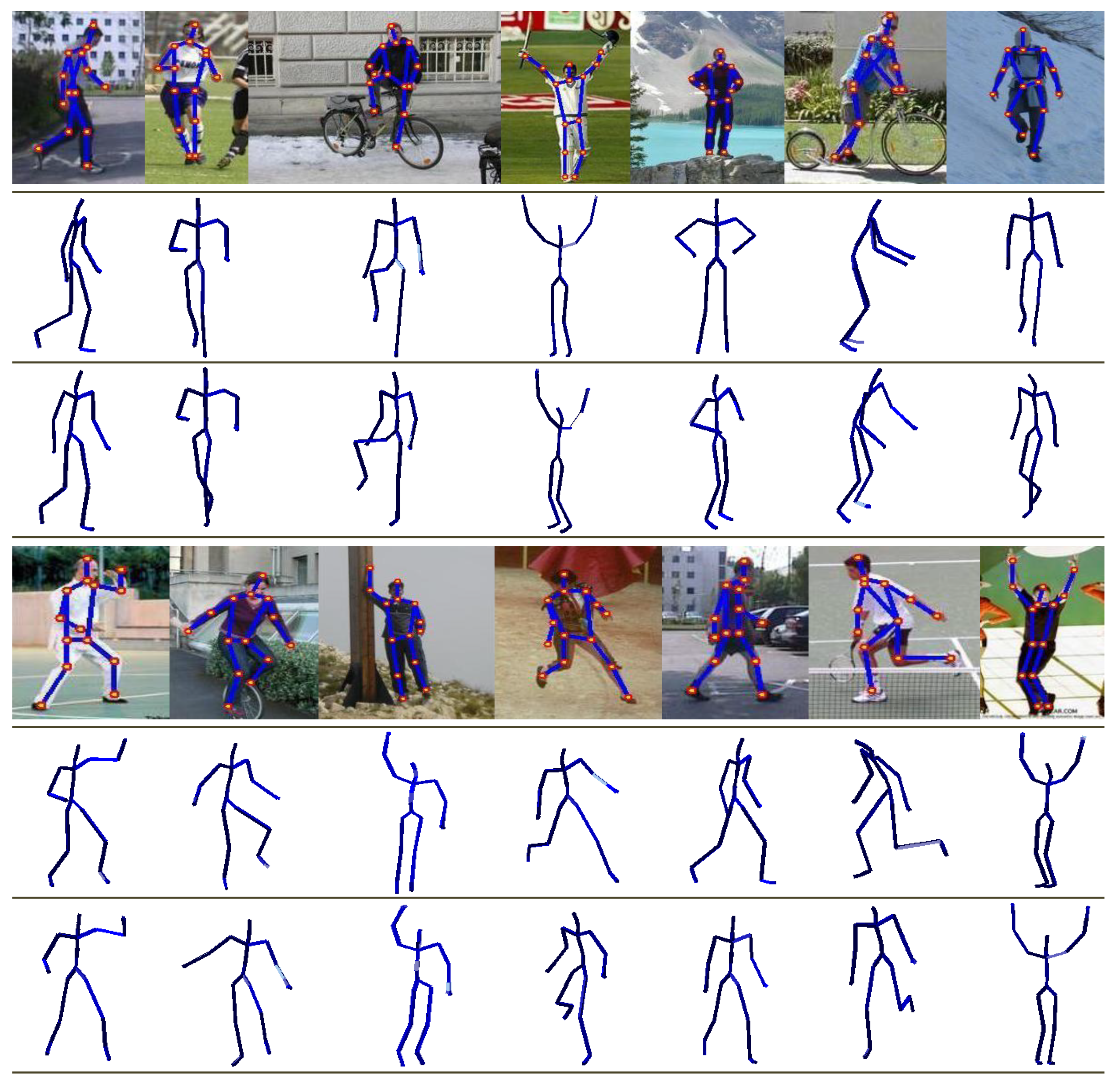
4.5.1. Real Images of Parse Dataset
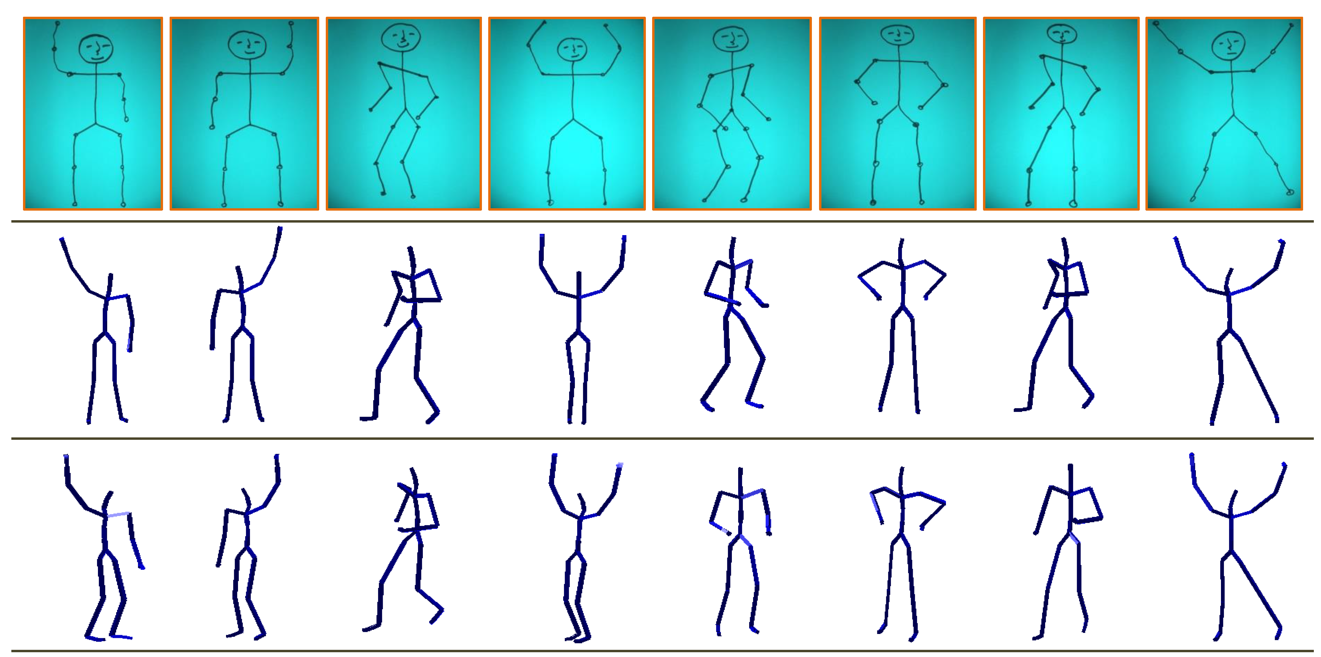
4.5.2. Hand-Drawn Sketches
4.6. Controlled Experiments
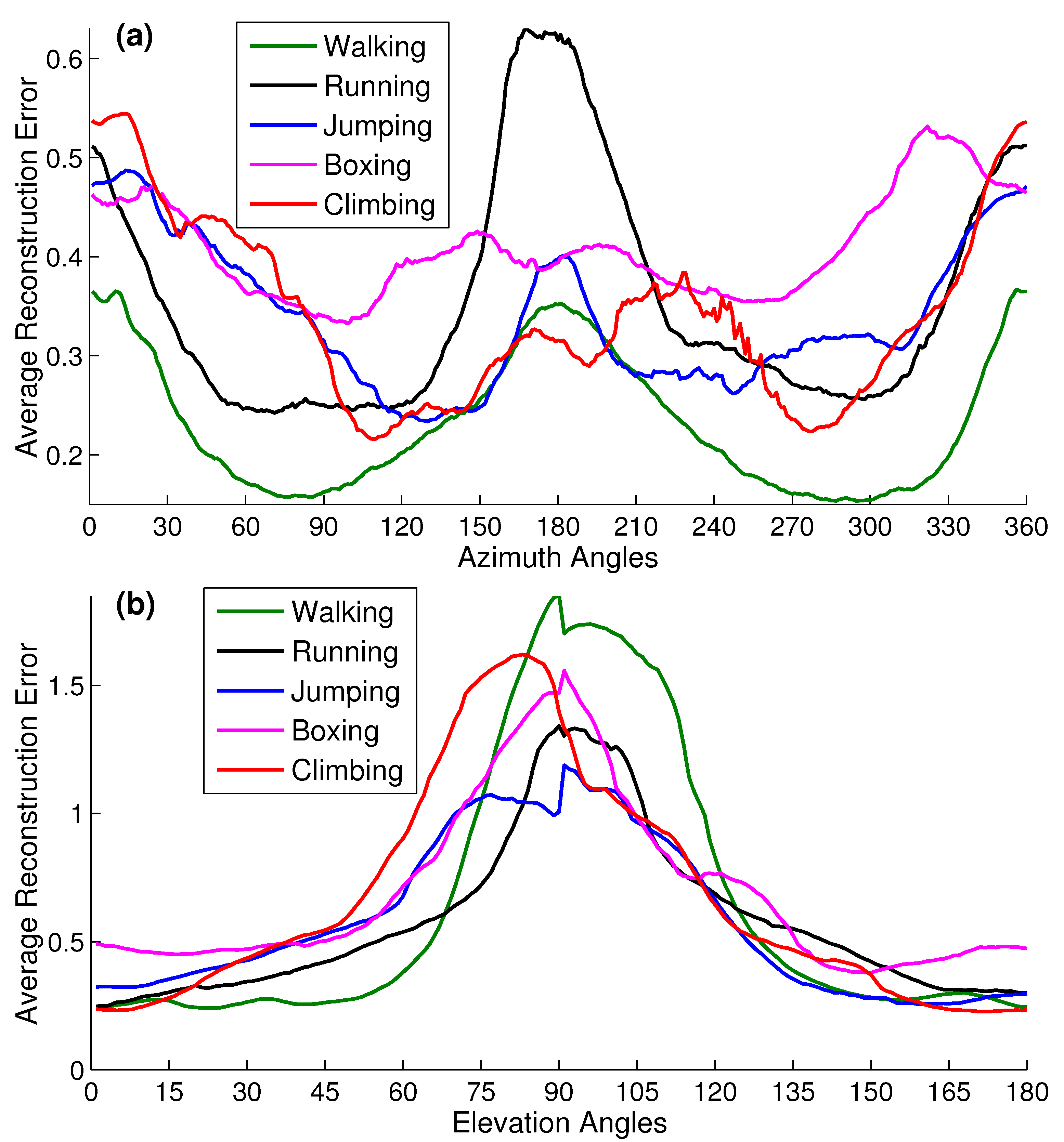
4.6.1. Camera Viewpoints
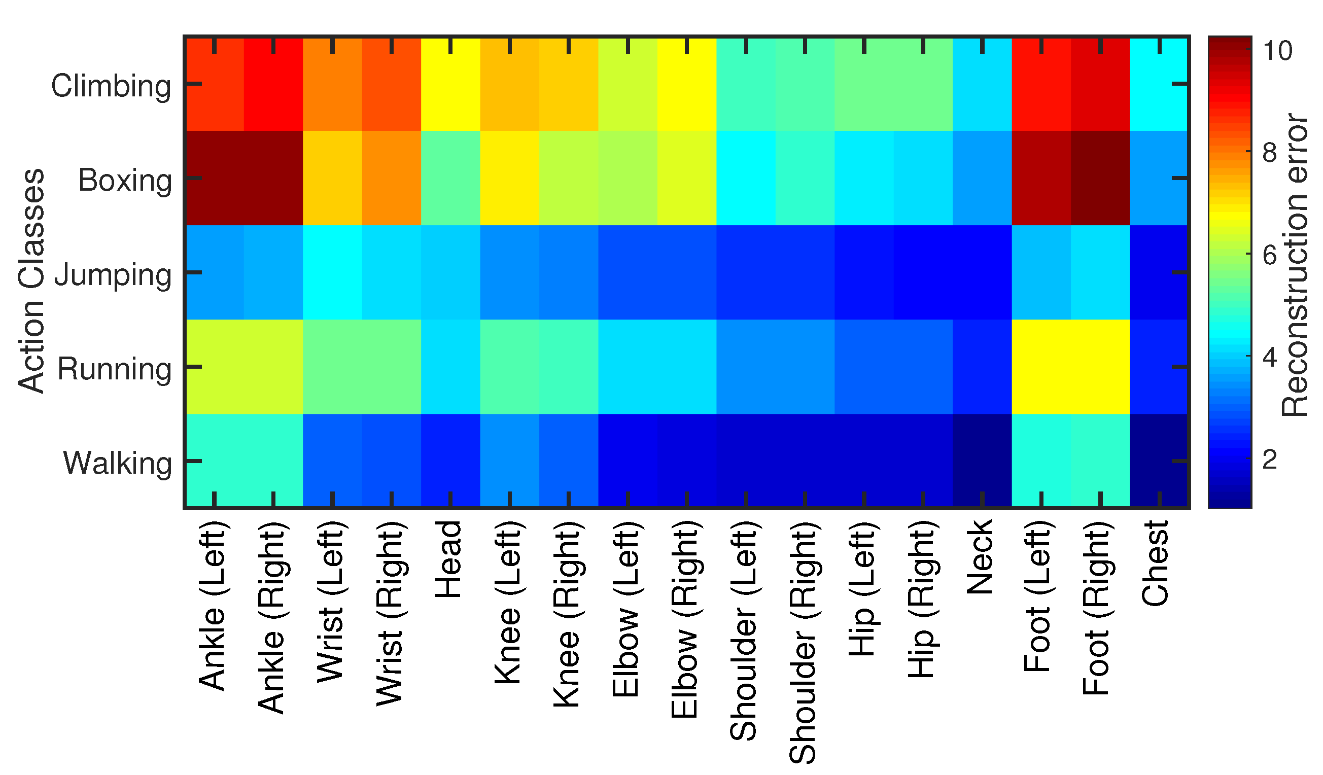
4.6.2. Joints’ Sensitivity
5. Conclusions
Author Contributions
Funding
Institutional Review Board Statement
Informed Consent Statement
Data Availability Statement
Conflicts of Interest
References
- Yasin, H.; Hussain, M.; Weber, A. Keys for Action: An Efficient Keyframe-Based Approach for 3D Action Recognition Using a Deep Neural Network. Sensors 2020, 20, 2226. [Google Scholar] [CrossRef]
- An, K.N.; Jacobsen, M.; Berglund, L.; Chao, E. Application of a magnetic tracking device to kinesiologic studies. J. Biomech. 1988, 21, 613–620. [Google Scholar] [CrossRef]
- Raskar, R.; Nii, H.; deDecker, B.; Hashimoto, Y.; Summet, J.; Moore, D.; Zhao, Y.; Westhues, J.; Dietz, P.; Barnwell, J.; et al. Prakash: Lighting Aware Motion Capture Using Photosensing Markers and Multiplexed Illuminators. ACM Trans. Graph. 2007, 26. [Google Scholar] [CrossRef]
- VICONPEAK. Camera MX 40. 2006. Available online: http://www.vicon.com/products/mx40.html (accessed on 20 November 2020).
- PHASE SPACE INC. Impulse Camera. 2007. Available online: http://www.phasespace.com (accessed on 18 November 2020).
- Pons-Moll, G.; Fleet, D.J.; Rosenhahn, B. Posebits for Monocular Human Pose Estimation. In Proceedings of the IEEE Conference on Computer Vision and Pattern Recognition (CVPR), Columbus, OH, USA, 23–28 June 2014. [Google Scholar]
- Rogez, G.; Schmid, C. MoCap-Guided Data Augmentation for 3D Pose Estimation in the Wild. In Proceedings of the 30th International Conference on Neural Information Processing Systems, NIPS’16, Barcelona, Spain, 4–9 December 2016. [Google Scholar]
- Yasin, H. Towards Efficient 3D Pose Retrieval and Reconstruction from 2D Landmarks. In Proceedings of the 2017 IEEE International Symposium on Multimedia (ISM), Taichung, Taiwan, 11–13 December 2017; pp. 169–176. [Google Scholar]
- Yang, W.; Ouyang, W.; Wang, X.; Ren, J.; Li, H.; Wang, X. 3D Human Pose Estimation in the Wild by Adversarial Learning. In Proceedings of the 2018 IEEE/CVF Conference on Computer Vision and Pattern Recognition, Salt Lake City, UT, USA, 18–23 June 2018. [Google Scholar]
- Yasin, H.; Iqbal, U.; Krüger, B.; Weber, A.; Gall, J. A Dual-Source Approach for 3D Pose Estimation from a Single Image. In Proceedings of the IEEE Conference on Computer Vision and Pattern Recognition (CVPR), Las Vegas, NV, USA, 27–30 June 2016. [Google Scholar]
- Zhou, X.; Huang, Q.; Sun, X.; Xue, X.; Wei, Y. Towards 3D Human Pose Estimation in the Wild: A Weakly-Supervised Approach. In Proceedings of the 2017 IEEE International Conference on Computer Vision (ICCV), Venice, Italy, 22–29 October 2017. [Google Scholar]
- Tome, D.; Russell, C.; Agapito, L. Lifting From the Deep: Convolutional 3D Pose Estimation From a Single Image. In Proceedings of the IEEE Conference on Computer Vision and Pattern Recognition (CVPR), Honolulu, HI, USA, 21–26 July 2017. [Google Scholar]
- Pavllo, D.; Feichtenhofer, C.; Grangier, D.; Auli, M. 3D Human Pose Estimation in Video With Temporal Convolutions and Semi-Supervised Training. In Proceedings of the IEEE/CVF Conference on Computer Vision and Pattern Recognition (CVPR), Long Beach, CA, USA, 15–20 June 2019. [Google Scholar]
- Sharma, S.; Varigonda, P.T.; Bindal, P.; Sharma, A.; Jain, A. Monocular 3D Human Pose Estimation by Generation and Ordinal Ranking. In Proceedings of the IEEE/CVF International Conference on Computer Vision (ICCV, Seoul, Korea, 27 October–2 November 2019. [Google Scholar]
- Wang, L.; Chen, Y.; Guo, Z.; Qian, K.; Lin, M.; Li, H.; Ren, J.S. Generalizing Monocular 3D Human Pose Estimation in the Wild. In Proceedings of the IEEE/CVF International Conference on Computer Vision Workshops (ICCVW), Seoul, Korea, 27–28 October 2019. [Google Scholar]
- CMU. CMU Motion Capture Database. 2003. Available online: http://mocap.cs.cmu.edu/ (accessed on 15 January 2020).
- Müller, M.; Röder, T.; Clausen, M.; Eberhardt, B.; Krüger, B.; Weber, A. Documentation Mocap Database HDM05; Technical Report CG-2007-2; Universität Bonn: Bonn, Germany, 2007. [Google Scholar]
- Ionescu, C.; Papava, D.; Olaru, V.; Sminchisescu, C. Human3.6M: Large Scale Datasets and Predictive Methods for 3D Human Sensing in Natural Environments. IEEE Trans. Pattern Anal. Mach. Intell. 2014, 36, 1325–1339. [Google Scholar] [CrossRef] [PubMed]
- Ramanan, D. Learning to parse images of articulated bodies. In Proceedings of the 19th International Conference on Neural Information Processing Systems (NIPS’06), Vancouver, BC, Canada, 4–7 December 2006. [Google Scholar]
- Chen, Y.; Chai, J. 3D Reconstruction of Human Motion and Skeleton from Uncalibrated Monocular Video. In Proceedings of the Asian Conference on Computer Vision (ACCV), Xi’an, China, 23–27 September 2009. [Google Scholar]
- Akhter, I.; Black, M.J. Pose-Conditioned Joint Angle Limits for 3D Human Pose Reconstruction. In Proceedings of the IEEE Conference on Computer Vision and Pattern Recognition (CVPR), Boston, MA, USA, 7–12 June 2015. [Google Scholar]
- Pons-Moll, G.; Baak, A.; Gall, J.; Leal-Taixe, L.; Mueller, M.; Seidel, H.P.; Rosenhahn, B. Outdoor Human Motion Capture using Inverse Kinematics and von Mises-Fisher Sampling. In Proceedings of the IEEE International Conference on Computer Vision (ICCV), Barcelona, Spain, 6–13 November 2011. [Google Scholar]
- Sminchisescu, C.; Kanaujia, A.; Li, Z.; Metaxas, D.N. Discriminative Density Propagation for 3D Human Motion Estimation. In Proceedings of the IEEE Conference on Computer Vision and Pattern Recognition (CVPR), San Diego, CA, USA, 20–25 June 2005. [Google Scholar]
- Agarwal, A.; Triggs, B. Recovering 3D Human Pose from Monocular Images. Trans. Pattern Anal. Mach. Intell. 2005, 28, 44–58. [Google Scholar] [CrossRef] [PubMed]
- Bo, L.; Sminchisescu, C. Twin Gaussian Processes for Structured Prediction. Int. J. Comput. Vision 2010, 87, 27–52. [Google Scholar] [CrossRef]
- Yu, T.; Kim, T.; Cipolla, R. Unconstrained Monocular 3D Human Pose Estimation by Action Detection and Cross-Modality Regression Forest. In Proceedings of the IEEE Conference on Computer Vision and Pattern Recognition (CVPR), Portland, OR, USA, 23–28 June 2013. [Google Scholar]
- Li, S.; Chan, A.B. 3D Human Pose Estimation from Monocular Images with Deep Convolutional Neural Network. In Proceedings of the Asian Conference on Computer Vision (ACCV), Singapore, 1–5 November 2014. [Google Scholar]
- Li, S.; Zhang, W.; Chan, A. Maximum-Margin Structured Learning with Deep Networks for 3D Human Pose Estimation. In Proceedings of the IEEE International Conference on Computer Vision (ICCV), Santiago, Chile, 7–13 December 2015. [Google Scholar]
- Bo, L.; Sminchisescu, C.; Kanaujia, A.; Metaxas, D. Fast algorithms for large scale conditional 3D prediction. In Proceedings of the IEEE Conference on Computer Vision and Pattern Recognition (CVPR), Anchorage, AK, USA, 23–28 June 2008. [Google Scholar]
- Mori, G.; Malik, J. Recovering 3d human body configurations using shape contexts. Trans. Pattern Anal. Mach. Intell. 2006, 28, 1052–1062. [Google Scholar] [CrossRef] [PubMed]
- Mehta, D.; Sridhar, S.; Sotnychenko, O.; Rhodin, H.; Shafiei, M.; Seidel, H.P.; Xu, W.; Casas, D.; Theobalt, C. VNect: Real-time 3D Human Pose Estimation with a Single RGB Camera. ACM Trans. Graph. 2017, 36, 1–4. [Google Scholar] [CrossRef]
- Tekin, B.; Marquez-Neila, P.; Salzmann, M.; Fua, P. Learning to Fuse 2D and 3D Image Cues for Monocular Body Pose Estimation. In Proceedings of the IEEE International Conference on Computer Vision (ICCV), Venice, Italy, 22–29 October 2017. [Google Scholar]
- Simo-Serra, E.; Quattoni, A.; Torras, C.; Moreno-Noguer, F. A Joint Model for 2D and 3D Pose Estimation from a Single Image. In Proceedings of the IEEE Conference on Computer Vision and Pattern Recognition (CVPR), Portland, OR, USA, 23–28 June 2013. [Google Scholar]
- Kostrikov, I.; Gall, J. Depth Sweep Regression Forests for Estimating 3D Human Pose from Images. In Proceedings of the British Machine Vision Conference (BMVC), Nottingham, UK, 1–5 September 2014. [Google Scholar]
- Ramakrishna, V.; Kanade, T.; Sheikh, Y.A. Reconstructing 3D Human Pose from 2D Image Landmarks. In Proceedings of the European Conference on Computer Vision (ECCV), Florence, Italy, 7–13 October 2012. [Google Scholar]
- Fan, X.; Zheng, K.; Zhou, Y.; Wang, S. Pose Locality Constrained Representation for 3D Human Pose Reconstruction. In Proceedings of the European Conference on Computer Vision (ECCV), Zurich, Switzerland, 5–12 September 2014. [Google Scholar]
- Wang, C.; Wang, Y.; Lin, Z.; Yuille, A.L.; Gao, W. Robust Estimation of 3D Human Poses from a Single Image. In Proceedings of the IEEE Conference on Computer Vision and Pattern Recognition (CVPR), Columbus, OH, USA, 23–28 June 2014. [Google Scholar]
- Yang, Y.; Ramanan, D. Articulated Pose Estimation with Flexible Mixtures-of-parts. In Proceedings of the IEEE Conference on Computer Vision and Pattern Recognition (CVPR), Colorado Springs, CO, USA, 20–25 June 2011. [Google Scholar]
- Kanazawa, A.; Black, M.J.; Jacobs, D.W.; Malik, J. End-to-End Recovery of Human Shape and Pose. In Proceedings of the 2018 IEEE/CVF Conference on Computer Vision and Pattern Recognition, Salt Lake City, UT, USA, 18–23 June 2018. [Google Scholar]
- Chai, J.; Hodgins, J.K. Performance animation from low-dimensional control signals. ACM Trans. Graph. (ToG) 2005, 24, 686–696. [Google Scholar] [CrossRef]
- Tautges, J.; Zinke, A.; Krüger, B.; Baumann, J.; Weber, A.; Helten, T.; Müller, M.; Seidel, H.P.; Eberhardt, B. Motion reconstruction using sparse accelerometer data. ACM Trans. Graph. (ToG) 2011, 30. [Google Scholar] [CrossRef]
- Jain, E.; Sheikh, Y.; Mahler, M.; Hodgins, J. Three-dimensional proxies for hand-drawn characters. ACM Trans. Graph. (ToG) 2012, 31. [Google Scholar] [CrossRef]
- Yasin, H.; Krüger, B.; Weber, A. Model based Full Body Human Motion Reconstruction from Video Data. In Proceedings of the 6th International Conference on Computer Vision/Computer Graphics Collaboration Techniques and Applications (MIRAGE), Berlin, Germany, 6–7 June 2013. [Google Scholar]
- Hornung, A.; Dekkers, E.; Kobbelt, L. Character Animation from 2D Pictures and 3D Motion Data. ACM Trans. Graph. (ToG) 2007, 26. [Google Scholar] [CrossRef]
- Bălan, A.O.; Sigal, L.; Black, M.J.; Davis, J.E.; Haussecker, H.W. Detailed human shape and pose from images. In Proceedings of the IEEE Conference on Computer Vision and Pattern Recognition (CVPR), Minneapolis, MN, USA, 17–22 June 2007. [Google Scholar]
- Simo-Serra, E.; Ramisa, A.; Alenyà, G.; Torras, C.; Moreno-Noguer, F. Single Image 3D Human Pose Estimation from Noisy Observations. In Proceedings of the IEEE Conference on Computer Vision and Pattern Recognition (CVPR), Providence, RI, USA, 16–21 June 2012. [Google Scholar]
- Iqbal, U.; Doering, A.; Yasin, H.; Krüger, B.; Weber, A.; Gall, J. A dual-source approach for 3D human pose estimation from single images. Comput. Vis. Image Underst. 2018, 172, 37–49. [Google Scholar] [CrossRef]
- Zhou, S.; Jiang, M.; Wang, Q.; Lei, Y. Towards Locality Similarity Preserving to 3D Human Pose Estimation. In Proceedings of the Asian Conference on Computer Vision (ACCV), Kyoto, Japan, 30 November–4 December 2020. [Google Scholar]
- Chen, C.; Ramanan, D. 3D Human Pose Estimation = 2D Pose Estimation + Matching. In Proceedings of the 2017 IEEE Conference on Computer Vision and Pattern Recognition (CVPR), Honolulu, HI, USA, 21–26 July 2017; pp. 5759–5767. [Google Scholar]
- Valmadre, J.; Lucey, S. Deterministic 3D Human Pose Estimation Using Rigid Structure. In Proceedings of the European Conference on Computer Vision (ECCV), Crete, Greece, 5–11 September 2010. [Google Scholar]
- Wei, X.K.; Chai, J. Modeling 3D human poses from uncalibrated monocular images. In Proceedings of the International Conference on Computer Vision (ICCV), Kyoto, Japan, 27 September–4 October 2009. [Google Scholar]
- Baak, A.; Muller, M.; Bharaj, G.; Seidel, H.P.; Theobalt, C. A Data-driven Approach for Real-time Full Body Pose Reconstruction from a Depth Camera. In Proceedings of the International Conference on Computer Vision (ICCV), Barcelona, Spain, 6–13 November 2011. [Google Scholar]
- Shotton, J.; Fitzgibbon, A.; Cook, M.; Sharp, T.; Finocchio, M.; Moore, R.; Kipman, A.; Blake, A. Real-time Human Pose Recognition in Parts from Single Depth Images. In Proceedings of the IEEE Conference on Computer Vision and Pattern Recognition (CVPR), Colorado Springs, CO, USA, 20–25 June 2011. [Google Scholar]
- Shum, H.; Ho, E.S. Real-time Physical Modelling of Character Movements with Microsoft Kinect. In Proceedings of the 18th ACM Symposium on Virtual Reality Software and Technology (VRST), Toronto, Canada, 10–12 December 2012. [Google Scholar]
- Zhou, L.; Liu, Z.; Leung, H.; Shum, H.P.H. Posture Reconstruction Using Kinect with a Probabilistic Model. In Proceedings of the 20th ACM Symposium on Virtual Reality Software and Technology (VRST), Edinburgh, UK, 11–13 November 2014. [Google Scholar]
- Pavlakos, G.; Zhou, X.; Daniilidis, K. Ordinal Depth Supervision for 3D Human Pose Estimation. In Proceedings of the 2018 IEEE/CVF Conference on Computer Vision and Pattern Recognition, Salt Lake City, UT, USA, 18–23 June 2018. [Google Scholar]
- Shi, Y.; Han, X.; Jiang, N.; Zhou, K.; Jia, K.; Lu, J. FBI-Pose: Towards Bridging the Gap between 2D Images and 3D Human Poses using Forward-or-Backward Information. arXiv 2018, arXiv:1806.09241. [Google Scholar]
- Sedmidubsky, J.; Elias, P.; Zezula, P. Effective and efficient similarity searching in motion capture data. Multimed. Tools Appl. 2018, 77, 12073–12094. [Google Scholar] [CrossRef]
- Krüger, B.; Tautges, J.; Weber, A.; Zinke, A. Fast Local and Global Similarity Searches in Large Motion Capture Databases. In Proceedings of the ACM SIGGRAPH Symposium on Computer Animation (SCA), Madrid, Spain, 2–4 July 2010. [Google Scholar]
- Antol, S.; Zitnick, C.L.; Parikh, D. Zero-Shot Learning via Visual Abstraction. In Proceedings of the European Conference on Computer Vision (ECCV), Zurich, Switzerland, 6–12 September 2014. [Google Scholar]


| Synthetic 2D Input Testing Dataset (). | ||||||
|---|---|---|---|---|---|---|
| Components | Walking | Running | Jumping | Boxing | Climbing | Total |
| No. of human poses | 13,509 | 2970 | 5913 | 9128 | 12,289 | 43,809 |
| No. of subjects | 8 | 8 | 4 | 4 | 1 | 25 |
| Computational Efficiency in s for Feature Sets. | |||||
|---|---|---|---|---|---|
| Components | |||||
| (a) The development of the knowledge-base | 30.55 | 42.12 | 54.78 | 67.86 | 77.63 |
| (b) The construction of kd-tree | 97.60 | 118.12 | 130.26 | 144.49 | 197.73 |
| (c) The process of retrieval and reconstruction | 0.53 | 0.56 | 0.62 | 0.67 | 0.96 |
| Quantitative Evaluation on , , and . | |||||||
|---|---|---|---|---|---|---|---|
| Methods | Error Metrics | Walking | Running | Jumping | Boxing | Climbing | Average |
| (a) CMU MoCap dataset is used, | |||||||
| PCA (PC-18) | recon-err | 0.546 | 0.573 | 0.454 | 0.694 | 0.651 | 0.583 |
| recon-rate | 21.6% | 18.0% | 22.6% | 8.1% | 17.1% | 17.48% | |
| [35] | recon-err | 0.446 | 0.453 | 0.374 | 0.584 | 0.533 | 0.478 |
| recon-rate | 29.6% | 23.0% | 31.6% | 10.7% | 20.1% | 23.0% | |
| [36] | recon-err | 0.360 | 0.417 | 0.343 | 0.579 | 0.560 | 0.452 |
| recon-rate | 53.4% | 29.8% | 34.12% | 13.3% | 21.7% | 30.46% | |
| recon-err | 0.300 | 0.390 | 0.322 | 0.530 | 0.528 | 0.414 | |
| recon-rate | 71.2% | 35.1% | 39.5% | 17.0% | 27.9% | 38.14% | |
| recon-err | 0.260 | 0.385 | 0.316 | 0.535 | 0.522 | 0.404 | |
| recon-rate | 73.9% | 38.2% | 41.6% | 16.4% | 27.0% | 39.42% | |
| recon-err | 0.272 | 0.432 | 0.321 | 0.534 | 0.526 | 0.417 | |
| recon-rate | 70.4% | 34.0% | 40.2% | 16.8% | 28.1% | 37.9% | |
| [8] | recon-err | 0.195 | 0.286 | 0.196 | 0.396 | 0.409 | 0.296 |
| recon-rate | 84.7% | 62.1% | 84.5% | 45.1% | 40.6% | 63.4% | |
| Our App. | recon-err | 0.183 | 0.253 | 0.179 | 0.365 | 0.391 | 0.274 |
| recon-rate | 85.8% | 64.5% | 85.8% | 49.2% | 41.9% | 65.44% | |
| (b) CMU MoCap dataset is used, | |||||||
| Our App. | recon-err | 0.207 | 0.331 | 0.227 | 0.413 | 0.529 | 0.341 |
| recon-rate | 82.9% | 51.7% | 77.8% | 39.1% | 22.1% | 54.72% | |
| (c) HDM05 MoCap dataset is used, | |||||||
| [8] | recon-err | 0.317 | 0.406 | 0.237 | 0.554 | 0.595 | 0.422 |
| recon-rate | 54.9% | 29.3% | 85.4% | 6.4% | 17.6% | 38.7% | |
| Our App. | recon-err | 0.301 | 0.391 | 0.213 | 0.529 | 0.568 | 0.4 |
| recon-rate | 56.1% | 30.9% | 86.9% | 8.73% | 18.9% | 40.31% | |
| Quantitative Evaluation on . | ||||||||||||||||
|---|---|---|---|---|---|---|---|---|---|---|---|---|---|---|---|---|
| Methods | Dir. | Disc. | Eat | Greet | Ph. | Pose | Pur. | Sit | SitD. | Smoke | Photo | Wait | Walk | WalkD. | WalkT. | Mean |
| [47] | 51.9 | 45.3 | 62.4 | 55.7 | 49.2 | 56.0 | 46.4 | 56.3 | 76.6 | 58.8 | 79.1 | 58.9 | 35.6 | 63.4 | 46.3 | 56.1 |
| [10] | 60.0 | 54.7 | 71.6 | 67.5 | 63.8 | 61.9 | 55.7 | 73.9 | 110.8 | 78.9 | 96.9 | 67.9 | 47.5 | 89.3 | 53.4 | 70.5 |
| [49] | 53.3 | 46.8 | 58.6 | 61.2 | 56.0 | 58.1 | 48.9 | 55.6 | 73.4 | 60.3 | 76.1 | 62.2 | 35.8 | 61.9 | 51.1 | 57.5 |
| [48] | 59.1 | 63.3 | 70.6 | 65.1 | 61.2 | 73.2 | 83.7 | 84.9 | 72.7 | 84.3 | 68.4 | 81.9 | 57.5 | 75.1 | 49.6 | 70.0 |
| Our App. | 50.5 | 42.7 | 60.7 | 54.9 | 48.1 | 54.1 | 44.8 | 55.7 | 73.6 | 57.1 | 77.6 | 57.3 | 33.5 | 62.2 | 43.8 | 54.4 |
| Quantitative Evaluation on Noisy Input Data. | ||||||
|---|---|---|---|---|---|---|
| Methods | Error Metrics | (0.0) | (0.1) | (0.2) | (0.3) | (0.4) |
| [36] | recon-err | 0.414 | 0.449 | 0.485 | 0.561 | 0.630 |
| recon-rate | 32.6% | 28.7% | 24.4% | 18.1% | 13.1% | |
| [35] | recon-err | 0.466 | 0.497 | 0.558 | 0.634 | 0.704 |
| recon-rate | 23.9% | 20.5% | 13.8% | 9.3% | 4.8% | |
| Our App. | recon-err | 0.271 | 0.326 | 0.431 | 0.524 | 0.617 |
| recon-rate | 67.3% | 52.9% | 38.1% | 34.9% | 33.8% | |
Publisher’s Note: MDPI stays neutral with regard to jurisdictional claims in published maps and institutional affiliations. |
© 2021 by the authors. Licensee MDPI, Basel, Switzerland. This article is an open access article distributed under the terms and conditions of the Creative Commons Attribution (CC BY) license (https://creativecommons.org/licenses/by/4.0/).
Share and Cite
Yasin, H.; Krüger, B. An Efficient 3D Human Pose Retrieval and Reconstruction from 2D Image-Based Landmarks. Sensors 2021, 21, 2415. https://doi.org/10.3390/s21072415
Yasin H, Krüger B. An Efficient 3D Human Pose Retrieval and Reconstruction from 2D Image-Based Landmarks. Sensors. 2021; 21(7):2415. https://doi.org/10.3390/s21072415
Chicago/Turabian StyleYasin, Hashim, and Björn Krüger. 2021. "An Efficient 3D Human Pose Retrieval and Reconstruction from 2D Image-Based Landmarks" Sensors 21, no. 7: 2415. https://doi.org/10.3390/s21072415
APA StyleYasin, H., & Krüger, B. (2021). An Efficient 3D Human Pose Retrieval and Reconstruction from 2D Image-Based Landmarks. Sensors, 21(7), 2415. https://doi.org/10.3390/s21072415