
Development of Coral Investigation System Based on Semantic Segmentation of Single-Channel Images

 , ,
, ,
Abstract
1. Introduction
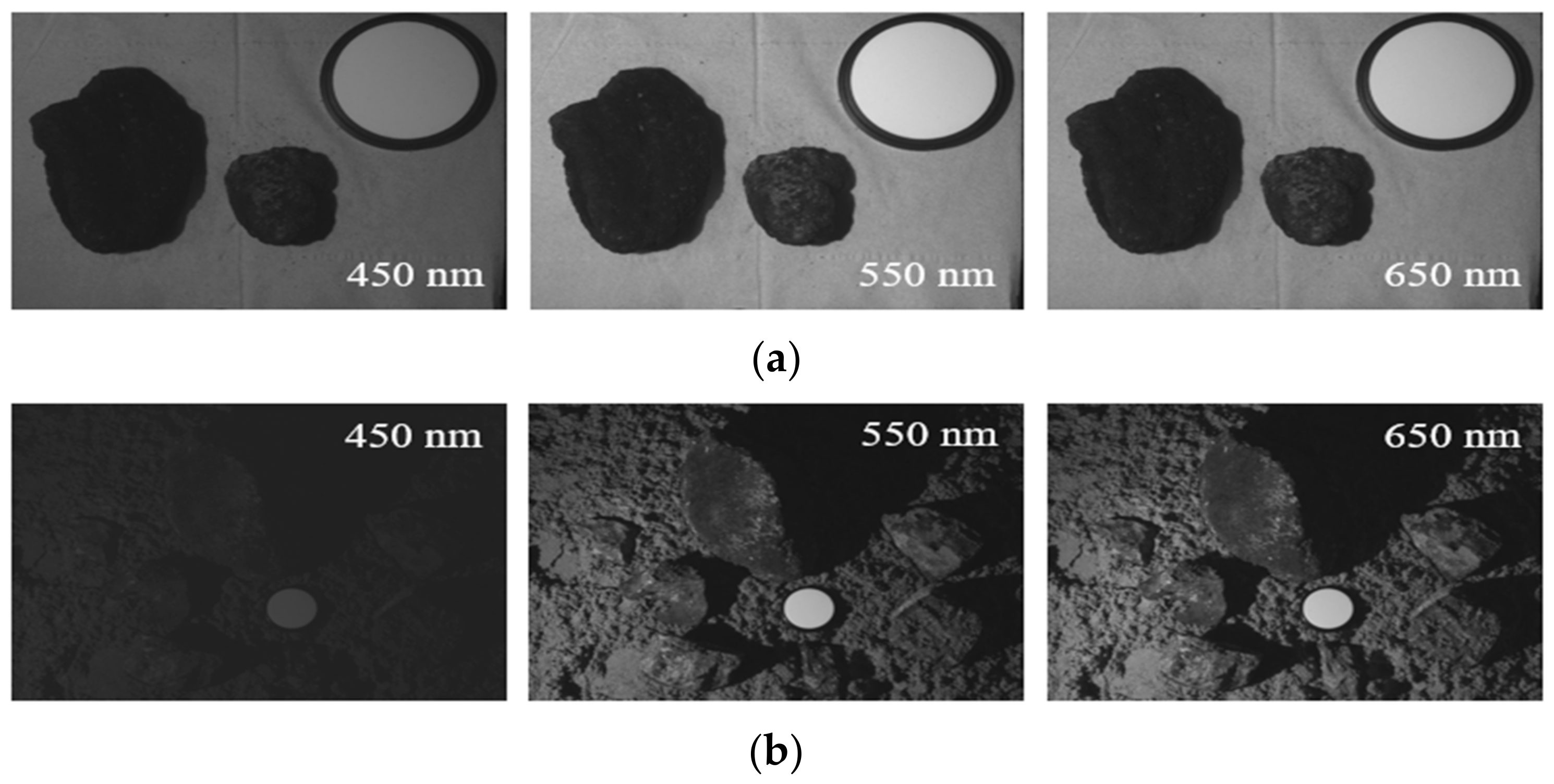
1.1. Segmentation Based on Spectral Features
1.2. Segmentation Based on RGB Image Features
- First, a new CoralS dataset containing single-channel underwater coral images collected in natural underwater environment was constructed using RGB and spectral imaging techniques, developed in laboratory.
- A deep CNN was modelled by fine-tuning deeplabv3+ model and adjusting ResNet34 backbone architecture for semantic segmentation of single-channel coral images. Depth to space module is added to the network to cope with the processing speed and memory usage of graphic processing unit (GPU).
- CAM module was installed at the tail of CNN to enhance visualization of the model’s segmentation effects.
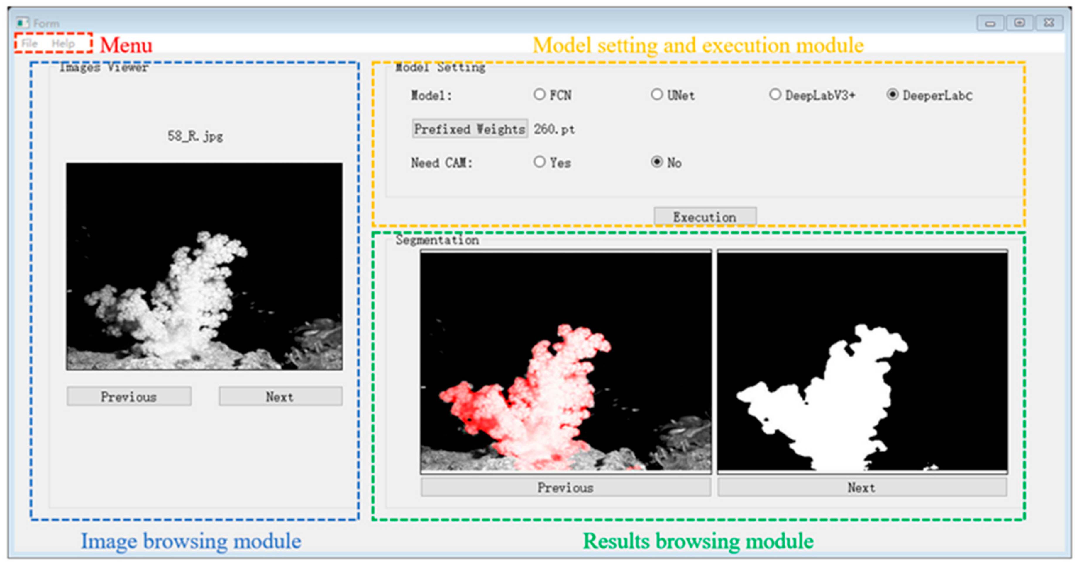
- The fourth contribution is a comparison of the developed model, using the CoralS dataset, to benchmark CNN models; results showed that the proposed model achieved high accuracy. The comparison can be visualized through a GUI developed to perform coral image segmentation.
2. Methodology
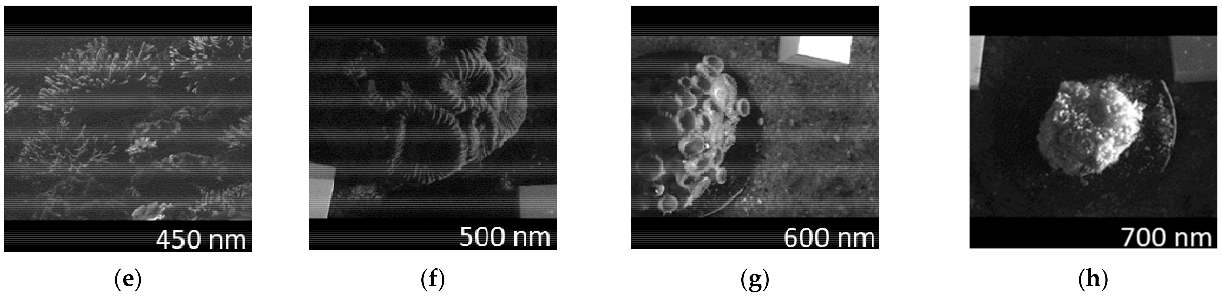
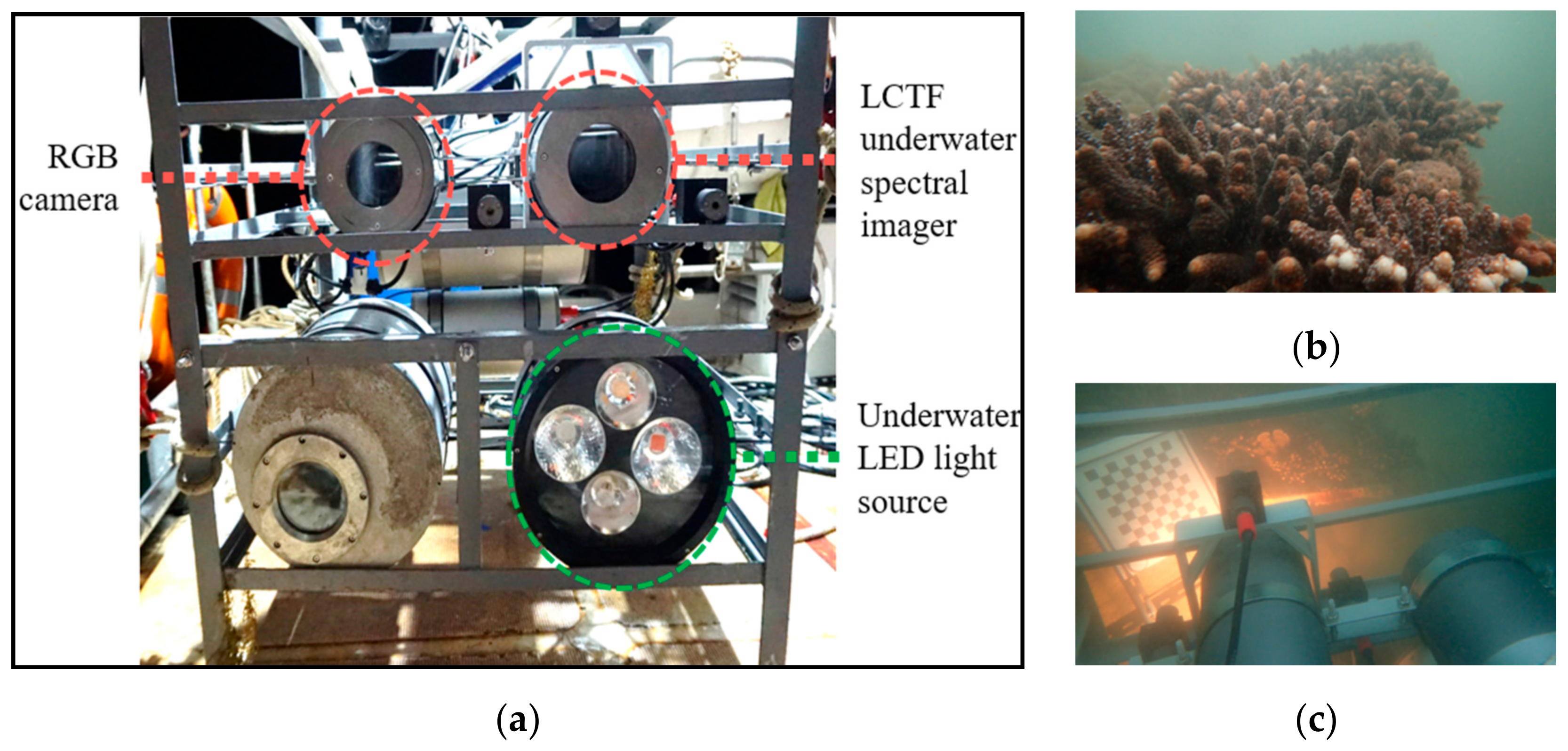
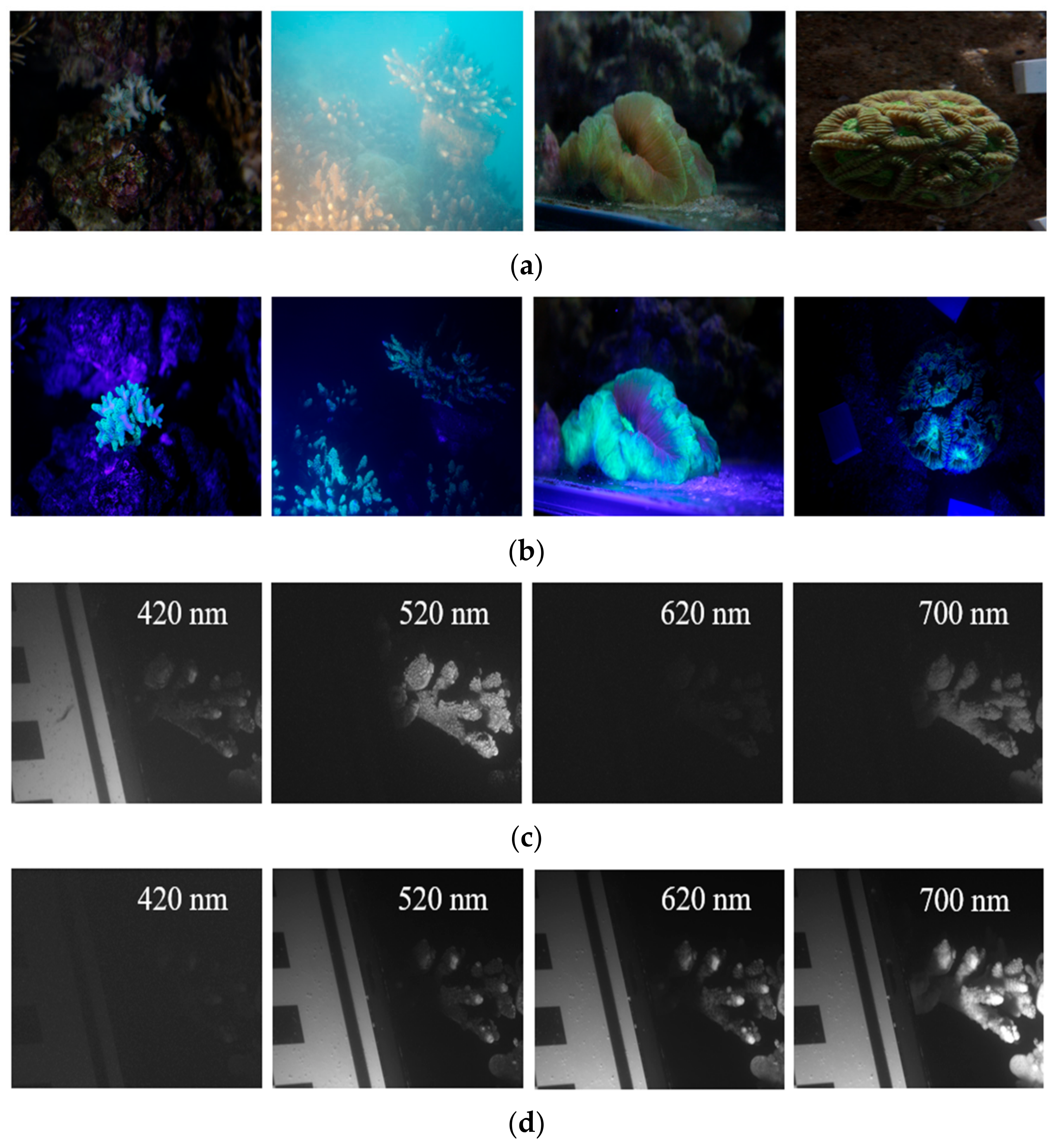
2.1. CoralS Dataset Collection
- ImageCrawler: obtain HTTP path of desired images;
- ImageDownloader: download images to a local directory.
- engine: Baidu;
- keyword: Corals, Dead coral skeleton, and Acropora;
- n_scroll: It defines the number of scrolling in the browser;
- link_save_dir: It holds the directory to save web links of the images;
- image_save_dir: It defines a directory to save images on the local disk.
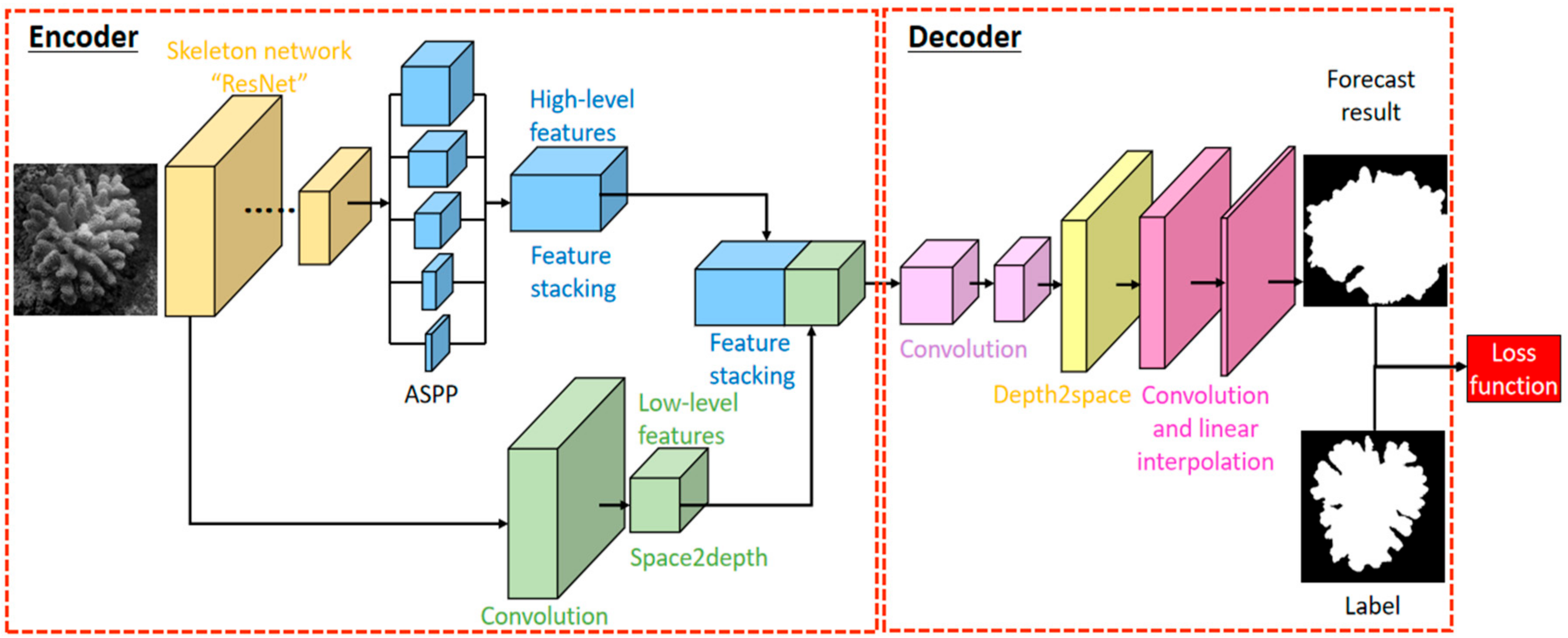
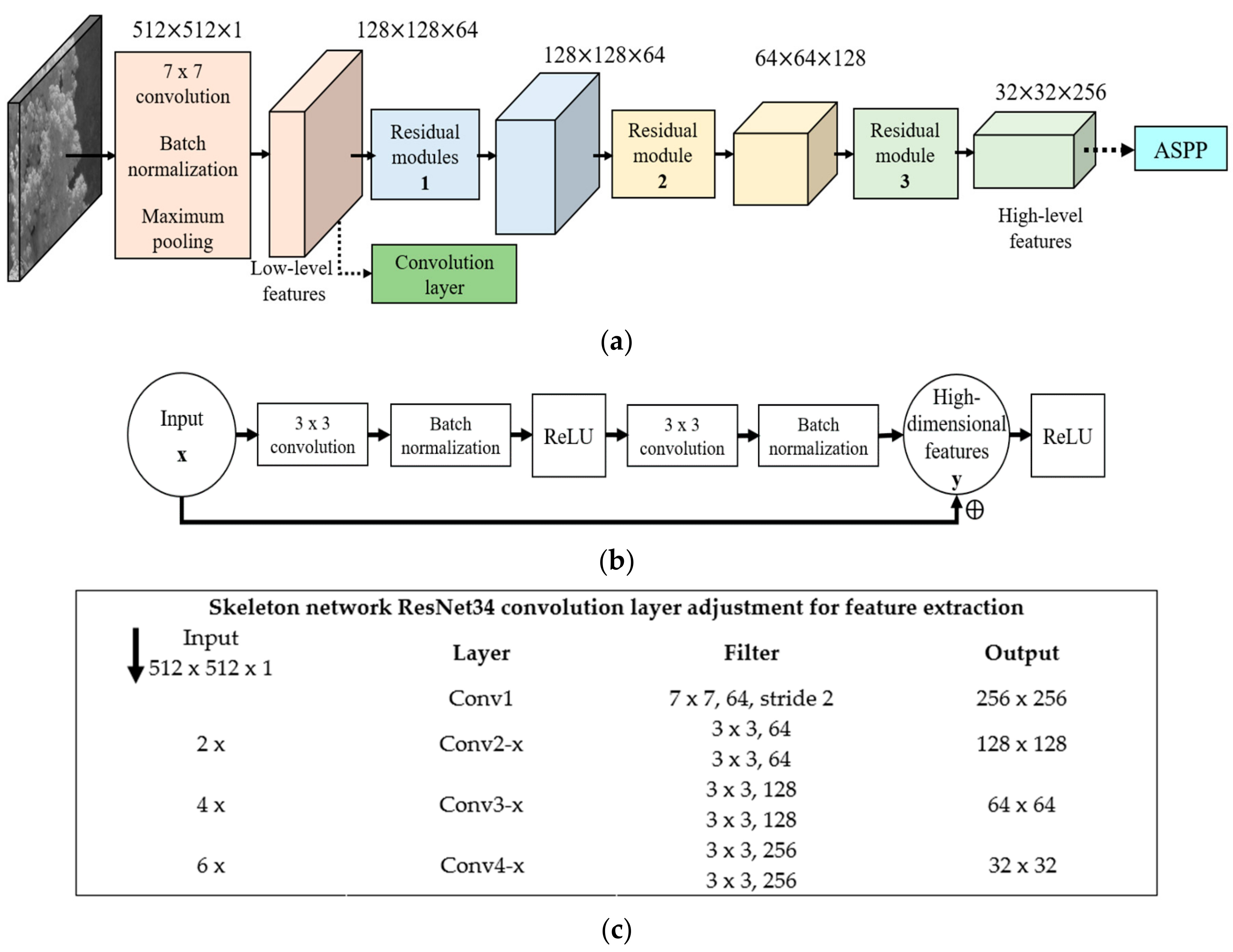
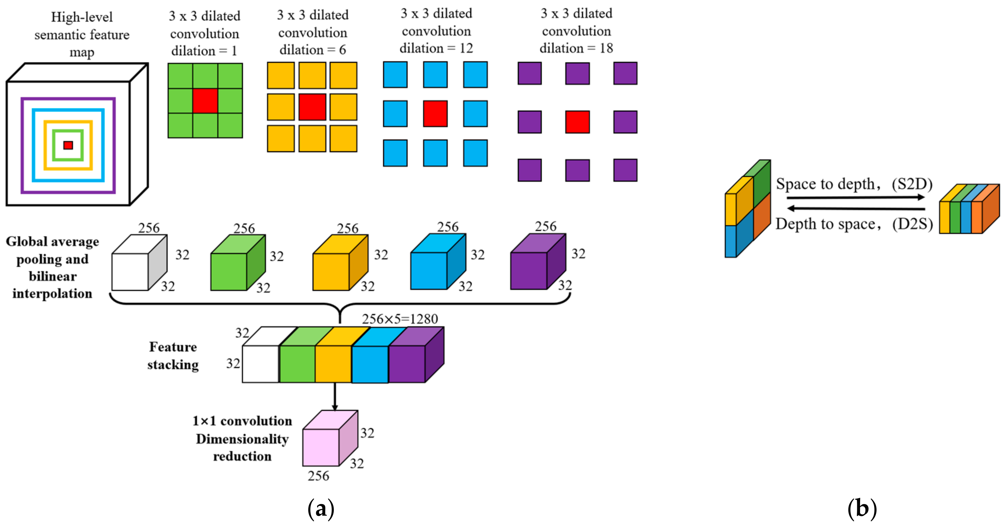
2.2. DeeperLabC Model
3. Experimentation
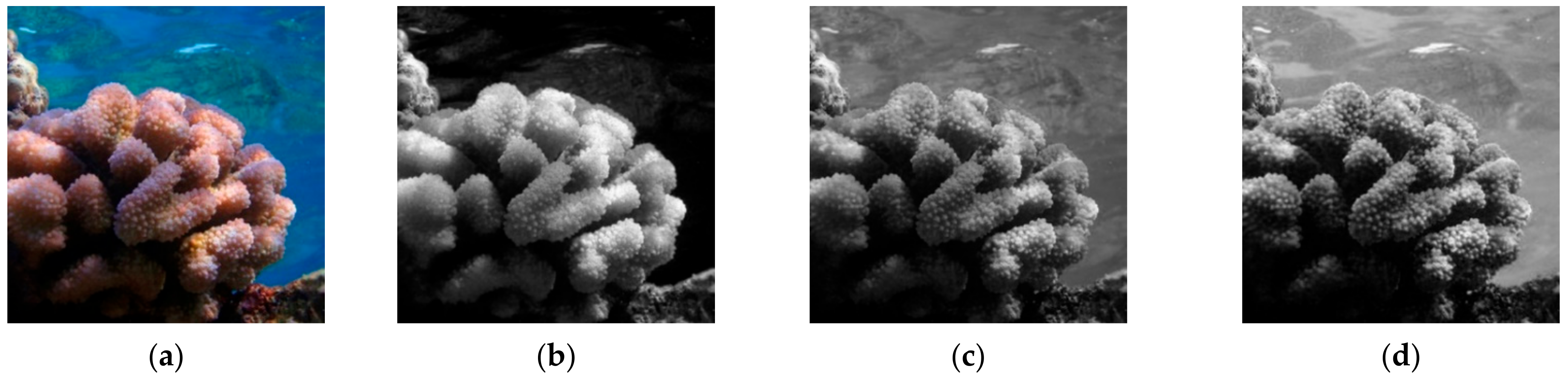
3.1. Data Preprocessing
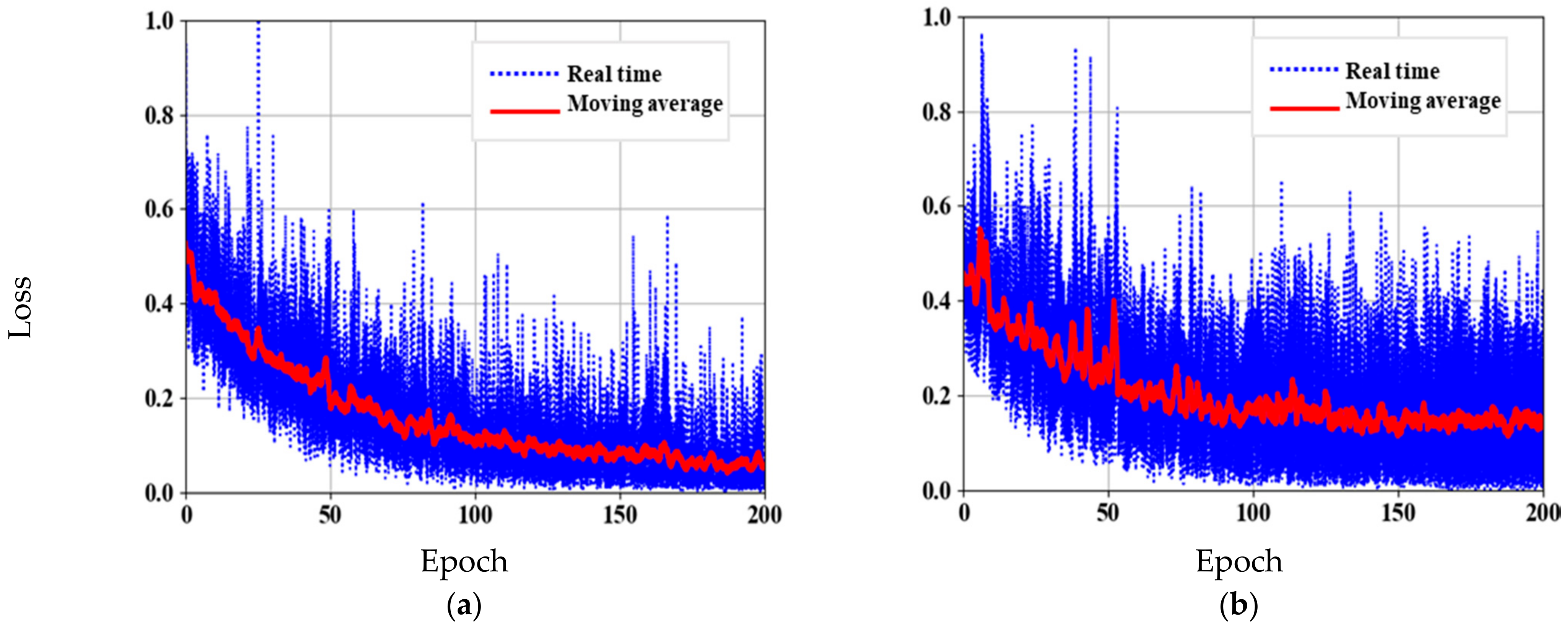
3.2. Skeleton Network Pre-Training
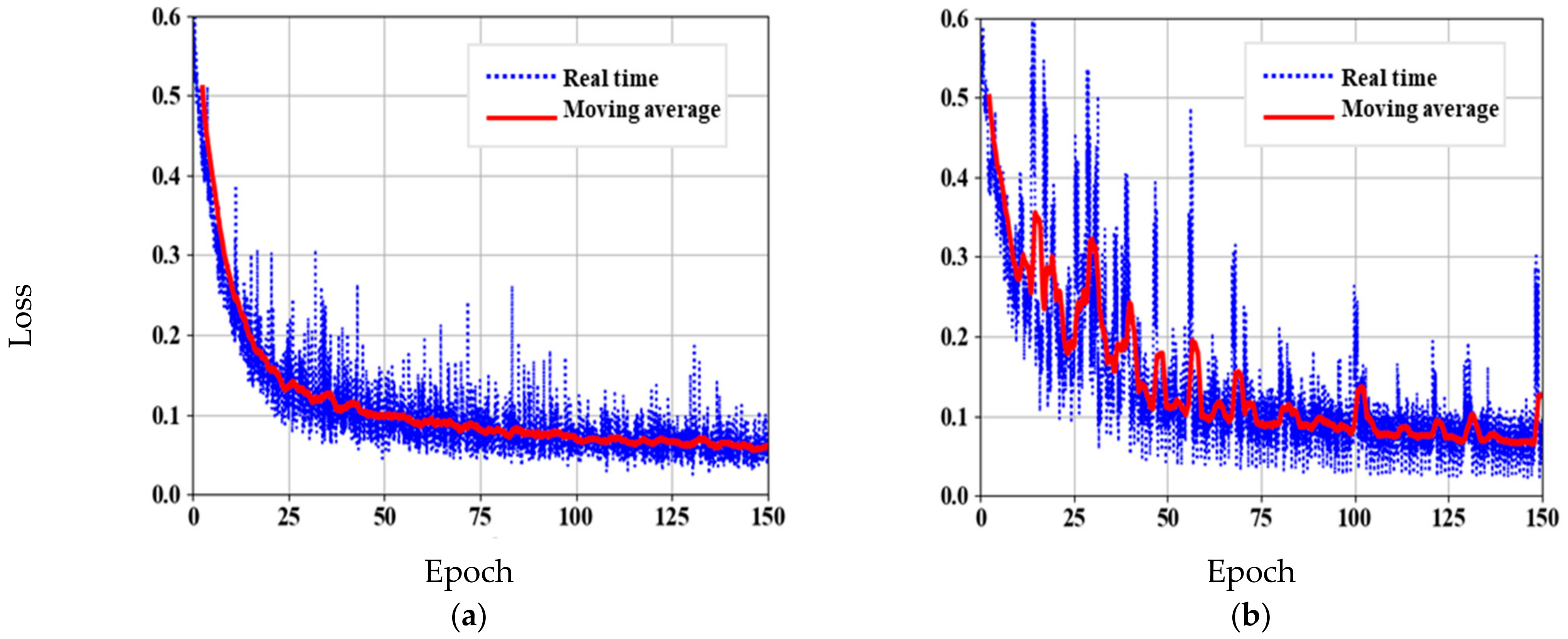
3.3. DeeperLabC Model Training
4. Results and Discussion
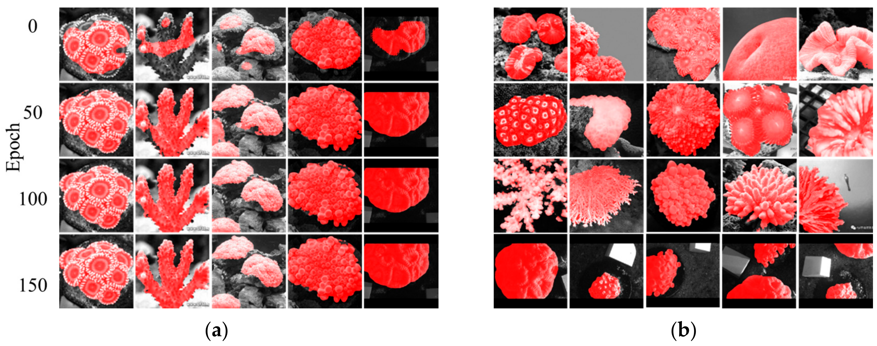
4.1. Visualization and Analysis of Segmentation Routine
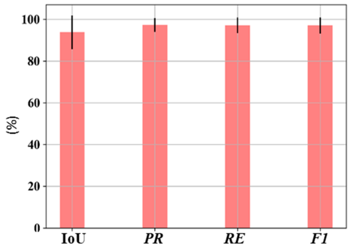
4.2. Performance Evaluation of Segmentation Model
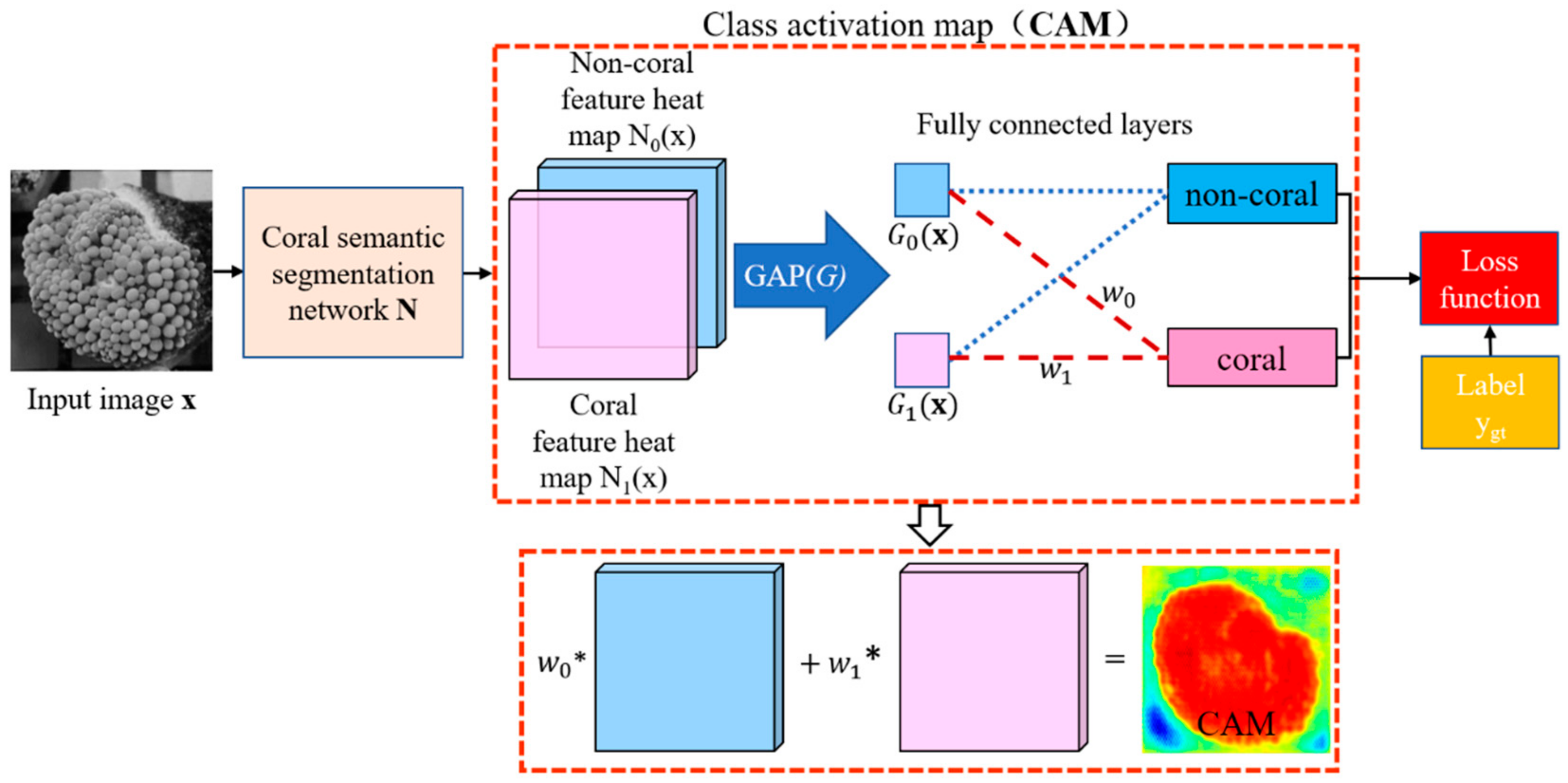
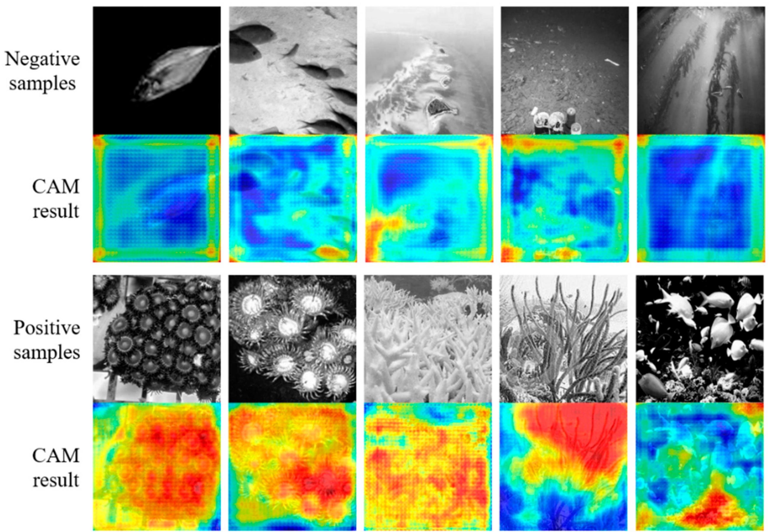
4.3. Visualization of Segmentation Based on CAM
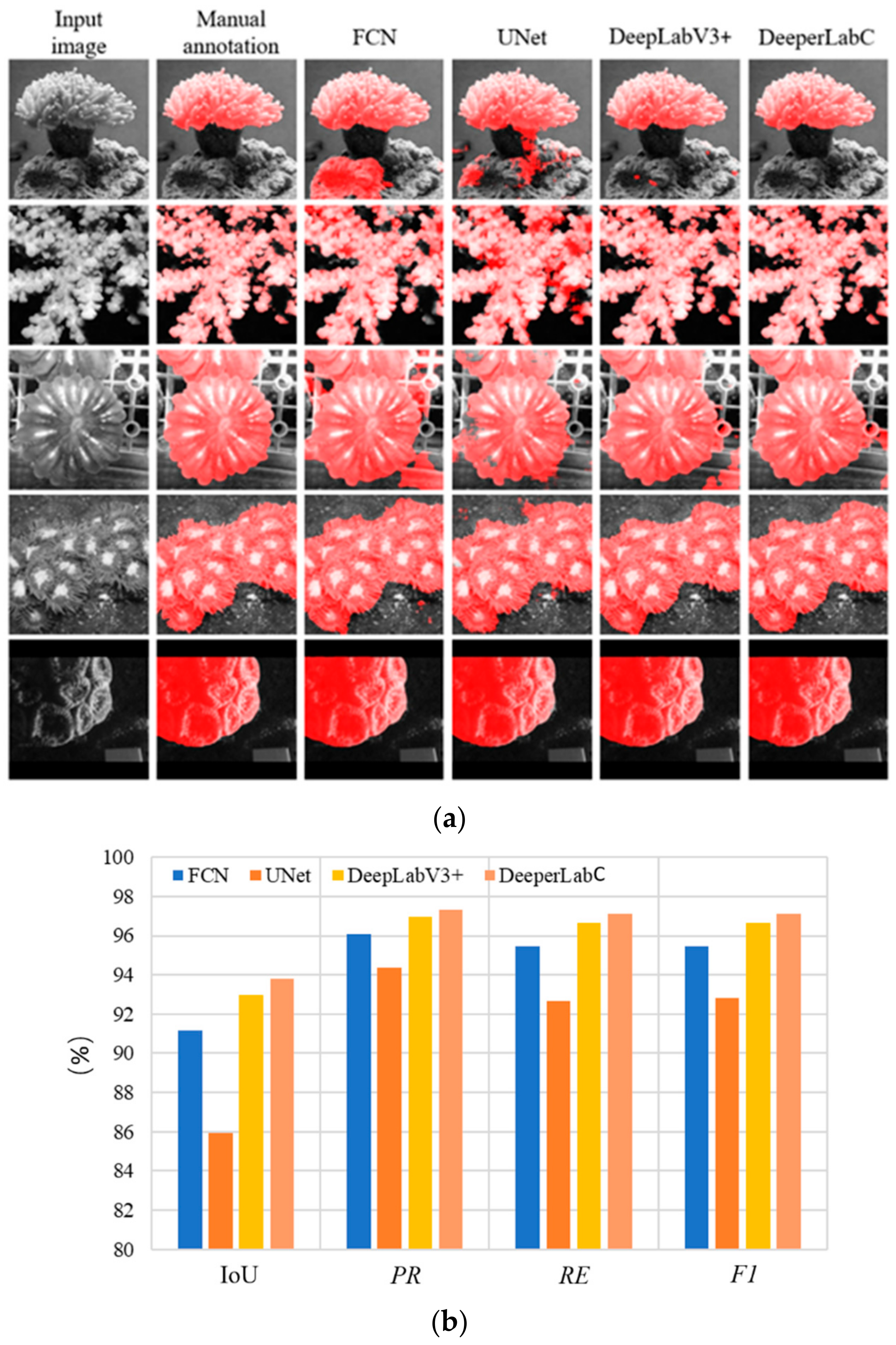
4.4. Comparison with Other Segmentation Models
5. Conclusions
Author Contributions
Funding
Institutional Review Board Statement
Informed Consent Statement
Data Availability Statement
Acknowledgments
Conflicts of Interest
Appendix A


Appendix B

References
- Coker, D.J.; Wilson, S.K.; Pratchett, M.S. Importance of live coral habitat for reef fishes. Rev. Fish. Biol. Fish. 2014, 24, 89–126. [Google Scholar] [CrossRef]
- Cole, A.J.; Pratchett, M.S.; Jones, G.P. Diversity and functional importance of coral-feeding fishes on tropical coral reefs. Fish. Fish. 2008, 9, 286–307. [Google Scholar] [CrossRef]
- Dearden, P.; Theberge, M.; Yasué, M. Using underwater cameras to assess the effects of snorkeler and SCUBA diver presence on coral reef fish abundance, family richness, and species composition. Environ. Monit. Assess. 2010, 163, 531–538. [Google Scholar] [CrossRef]
- Lirman, D.; Gracias, N.R.; Gintert, B.E.; Gleason, A.C.R.; Reid, R.P.; Negahdaripour, S.; Kramer, P. Development and application of a video-mosaic survey technology to document the status of coral reef communities. Environ. Monit. Assess. 2007, 125, 59–73. [Google Scholar] [CrossRef] [PubMed]
- Carleton, J.H.; Done, T.J. Quantitative video sampling of coral reef benthos: Large-scale application. Coral Reefs 1995, 14, 35–46. [Google Scholar] [CrossRef]
- Bertels, L.; Vanderstraete, T.; Coillie, S.; Knaeps, E.; Sterckx, S.; Goossens, R.; Deronde, B. Mapping of coral reefs using hyperspectral CASI data; a case study: Fordata, Tanimbar, Indonesia. Int. J. Remote Sens. 2008, 29, 2359–2391. [Google Scholar] [CrossRef]
- Bajjouk, T.; Mouquet, P.; Ropert, M.; Quod, J.P.; Hoarau, L.; Bigot, L.; Dantec, N.L.; Delacourt, C.; Populus, J. Detection of changes in shallow coral reefs status: Towards a spatial approach using hyperspectral and multispectral data. Ecol. Indic. 2019, 96, 174–191. [Google Scholar] [CrossRef]
- Hochberg, E. Spectral reflectance of coral reef bottom-types worldwide and implications for coral reef remote sensing. Remote Sens. Environ. 2003, 85, 159–173. [Google Scholar] [CrossRef]
- Beijbom, O.; Edmunds, P.J.; Roelfsema, C.; Smith, J.; Kline, D.I.; Neal, B.P.; Dunlap, M.J.; Moriarty, V.; Fan, T.Y.; Tan, C.J.; et al. Towards Automated Annotation of Benthic Survey Images: Variability of Human Experts and Operational Modes of Automation. PLoS ONE 2015, 10, e0130312. [Google Scholar]
- Guo, Y.; Liu, Y.; Oerlemans, A.; Lao, S.; Wu, S.; Lew, M.S. Deep learning for visual understanding: A review. Neurocomputing 2016, 187, 27–48. [Google Scholar] [CrossRef]
- Athanasios, V.; Doulamis, N.; Doulamis, A.; Protopapadakis, E. Deep learning for computer vision: A brief review. Comput. Intell. Neurosci. 2018, 2018, 7068349. [Google Scholar]
- Sharif, S.M.A.; Naqvi, R.A.; Biswas, M. Learning Medical Image Denoising with Deep Dynamic Residual Attention Network. Mathematics 2020, 8, 2192. [Google Scholar] [CrossRef]
- Naqvi, R.A.; Hussain, D.; Loh, W.K. Artificial Intelligence-Based Semantic Segmentation of Ocular Regions for Biometrics and Healthcare Applications. CMC-Comput. Mater. Con. 2021, 66, 715–732. [Google Scholar]
- Song, H.; Mehdi, S.R.; Huang, H.; Shahani, K.; Zhang, Y.; Raza, K.; Junaidullah; Khan, M.A. Classification of Freshwater Zooplankton by Pre-trained Convolutional Neural Network in Underwater Microscopy. Int. J. Adv. Comput. Sci. Appl. 2020, 11, 252–258. [Google Scholar]
- Hui, H.; Wang, C.; Liu, S.; Sun, Z.; Zhang, D.; Liu, C.; Jiang, Y.; Zhan, S.; Zhang, H.; Xu, R. Single spectral imagery and faster R-CNN to identify hazardous and noxious substances spills. Environ. Pollut. 2020, 258, 113688. [Google Scholar]
- Mogstad, A.A.; Johnsen, G. Spectral characteristics of coralline algae: A multi-instrumental approach, with emphasis on underwater hyperspectral imaging. Appl. Opt. 2017, 56, 9957–9975. [Google Scholar] [CrossRef]
- Foglini, F.; Angeletti, L.; Bracchi, V.; Chimienti, G.; Grande, V.; Hansen, I.M.; Meroni, A.N.; Marchese, F.; Mercorella, A.; Prampolini, M.; et al. Underwater Hyperspectral Imaging for seafloor and benthic habitat mapping. In Proceedings of the 2018 IEEE International Workshop on Metrology for the Sea, Learning to Measure Sea Health Parameters (MetroSea), Bari, Italy, 8–10 October 2018; pp. 201–205. [Google Scholar]
- Mogstad, A.A.; Johnsen, G.; Ludvigsen, M. Shallow-Water Habitat Mapping using Underwater Hyperspectral Imaging from an Unmanned Surface Vehicle: A Pilot Study. Remote Sens. 2019, 11, 685. [Google Scholar] [CrossRef]
- Letnes, P.A.; Hansen, I.M.; Aas, L.M.S.; Eide, I.; Pettersen, R.; Tassara, L.; Receveur, J.; Floch, S.L.; Guyomarch, J.; Camus, L.; et al. Underwater hyperspectral classification of deep-sea corals exposed to 2-methylnaphthalene. PLoS ONE 2019, 14, e0209960. [Google Scholar] [CrossRef] [PubMed]
- Otsu, N. A Threshold Selection Method from Gray-Level Histograms. IEEE Trans. Syst. Man Cybern. 1979, 9, 62–66. [Google Scholar] [CrossRef]
- Cuevas, E.; Zaldivar, D.; Cisneros, M.P. A novel multi-threshold segmentation approach based on differential evolution optimization. Expert Syst. Appl. 2010, 37, 5265–5271. [Google Scholar] [CrossRef]
- Chien, S.Y.; Huang, Y.W.; Hsieh, B.Y.; Ma, S.Y.; Chen, L.G. Fast Video Segmentation Algorithm with Shadow Cancellation, Global Motion Compensation, and Adaptive Threshold Techniques. IEEE Trans. Multimed. 2004, 6, 732–748. [Google Scholar] [CrossRef]
- Xu, Z.; Gao, G.; Hoffman, E.A.; Saha, P.K. Tensor scale-based anisotropic region growing for segmentation of elongated biological structures. In Proceedings of the 2012 9th IEEE International Symposium on Biomedical Imaging (ISBI), Barcelona, Spain, 2–5 May 2012; pp. 1032–1035. [Google Scholar]
- Shihavuddin, A.S.M.; Gracias, N.; Garcia, R.; Gleason, A.; Gintert, B. Image-Based Coral Reef Classification and Thematic Mapping. Remote Sens. 2013, 5, 1809–1841. [Google Scholar] [CrossRef]
- Kanopoulos, N.; Vasanthavada, N.; Baker, R.L. Design of an image edge detection filter using the Sobel operator. IEEE J. Solid-St. Circ. 1998, 23, 358–367. [Google Scholar] [CrossRef]
- Davis, L.S. A survey of edge detection techniques. Comput. Gr. Image Process. 1975, 4, 248–270. [Google Scholar] [CrossRef]
- Prewitt, J. Object enhancement and extraction. Picture Process. Psychopictorics 1970, 10, 15–19. [Google Scholar]
- Canny, J. A Computational Approach to Edge Detection. IEEE Trans. Pattern Anal. Mach. Intell. 1986, 8, 679–698. [Google Scholar] [CrossRef] [PubMed]
- Awalludin, E.A.; Hitam, M.S.; Yussof, W.N.J.H.W.; Bachok, Z. Modification of canny edge detection for coral reef components estimation distribution from underwater video transect. In Proceedings of the 2017 IEEE International Conference on Signal and Image Processing Applications (ICSIPA), Kuching, Malaysia, 12–14 September 2017; pp. 413–418. [Google Scholar]
- Krizhevsky, A.; Sutskever, I.; Hinton, G.E. ImageNet Classification with Deep Convolutional Neural Networks. In Advances in Neural Information Processing Systems 25; Pereira, F., Burges, C.J.C., Bottou, L., Weinberger, K.Q., Eds.; Curran Associates, Inc.: Red Hook, NY, USA, 2012; pp. 1097–1105. [Google Scholar]
- Simonyan, K.; Zisserman, A. Very Deep Convolutional Networks for Large-Scale Image Recognition. arXiv 2015, arXiv:1409.1556. [Google Scholar]
- He, K.; Zhang, X.; Ren, S.; Sun, J. Deep Residual Learning for Image Recognition. In Proceedings of the 2016 IEEE Conference on Computer Vision and Pattern Recognition (CVPR), Las Vegas, NV, USA, 27–30 June 2016; pp. 770–778. [Google Scholar]
- Huang, G.; Liu, Z.; Maaten, L.V.D.; Weinberger, K.Q. Densely Connected Convolutional Networks. In Proceedings of the 2017 IEEE Conference on Computer Vision and Pattern Recognition (CVPR), Honolulu, HI, USA, 21–26 July 2017; pp. 2261–2269. [Google Scholar]
- Long, J.; Shelhamer, E.; Darrell, T. Fully convolutional networks for semantic segmentation. In Proceedings of the 2015 IEEE Conference on Computer Vision and Pattern Recognition (CVPR), Boston, MA, USA, 7–12 June 2015; pp. 3431–3440. [Google Scholar]
- Ronneberger, O.; Fischer, P.; Brox, T. U-Net: Convolutional Networks for Biomedical Image Segmentation. In Medical Image Computing and Computer-Assisted Intervention—MICCAI 2015; Lecture Notes in Computer Science; Navab, N., Hornegger, J., Wells, W.M., Frangi, A.F., Eds.; Springer International Publishing: New York, NY, USA, 2015; pp. 234–241. [Google Scholar]
- Yu, F.; Koltun, V. Multi-Scale Context Aggregation by Dilated Convolutions. arXiv 2016, arXiv:1511.07122. [Google Scholar]
- Chen, L.C.; Papandreou, G.; Kokkinos, I.; Murphy, K.; Yuille, A.L. Semantic Image Segmentation with Deep Convolutional Nets and Fully Connected CRFs. arXiv 2016, arXiv:1412.7062. [Google Scholar]
- Chen, L.C.; Papandreou, G.; Kokkinos, I.; Murphy, K.; Yuille, A.L. DeepLab: Semantic Image Segmentation with Deep Convolutional Nets, Atrous Convolution, and Fully Connected CRFs. IEEE Trans. Pattern Anal. Mach. Intell. 2018, 40, 834–848. [Google Scholar] [CrossRef]
- Chen, L.C.; Papandreou, G.; Schroff, F.; Adam, H. Rethinking Atrous Convolution for Semantic Image Segmentation. arXiv 2017, arXiv:1706.05587. [Google Scholar]
- Chen, L.C.; Zhu, Y.; Papandreou, G.; Schroff, F.; Adam, H. Encoder-Decoder with Atrous Separable Convolution for Semantic Image Segmentation. In Computer Vision—ECCV 2018; Lecture Notes in Computer Science; Ferrari, V., Hebert, M., Sminchisescu, C., Weiss, Y., Eds.; Springer International Publishing: New York, NY, USA, 2018; Volume 11211, pp. 833–851. [Google Scholar]
- King, A.; Bhandarkar, S.M.; Hopkinson, B.M. A Comparison of Deep Learning Methods for Semantic Segmentation of Coral Reef Survey Images. In Proceedings of the 2018 IEEE/CVF Conference on Computer Vision and Pattern Recognition Workshops (CVPRW), Salt Lake City, UT, USA, 18–22 June 2018; pp. 1394–1402. [Google Scholar]
- Song, H.; Wan, Q.; Wu, C.; Shentu, Y.; Wang, W.; Yang, P.; Jia, W.; Li, H.; Huang, H.; Wang, H.; et al. Development of an underwater spectral imaging system based on LCTF. Infrared Laser Eng. 2020, 49, 0203005. [Google Scholar] [CrossRef]
- Yang, T.J.; Collins, M.D.; Zhu, Y.; Hwang, J.J.; Liu, T.; Zhang, X.; Sze, V.; Papandreou, G.; Chen, L.C. DeeperLab: Single-Shot Image Parser. arXiv 2019, arXiv:1902.05093. [Google Scholar]
- Zhou, B.; Khosla, A.; Lapedriza, A.; Oliva, A.; Torralba, A. Learning Deep Features for Discriminative Localization. In Proceedings of the 2016 IEEE Conference on Computer Vision and Pattern Recognition (CVPR), Las Vegas, NV, USA, 27–30 June 2016; pp. 2921–2929. [Google Scholar]
- Zuo, X.; Su, F.; Zhang, J.; Wu, W. Using Landsat Data to Detect Change in Live to Recently (<6 Months) Dead Coral Cover in the Western Xisha Islands, South China Sea. Sustainability 2020, 12, 5237. [Google Scholar]
- Dung, L.D. The status of coral reefs in central Vietnam’s coastal water under climate change. Aquat. Ecosyst. Health Manag. 2020, 23, 323–331. [Google Scholar] [CrossRef]


| Location | Coral Species | Reference Figure |
|---|---|---|
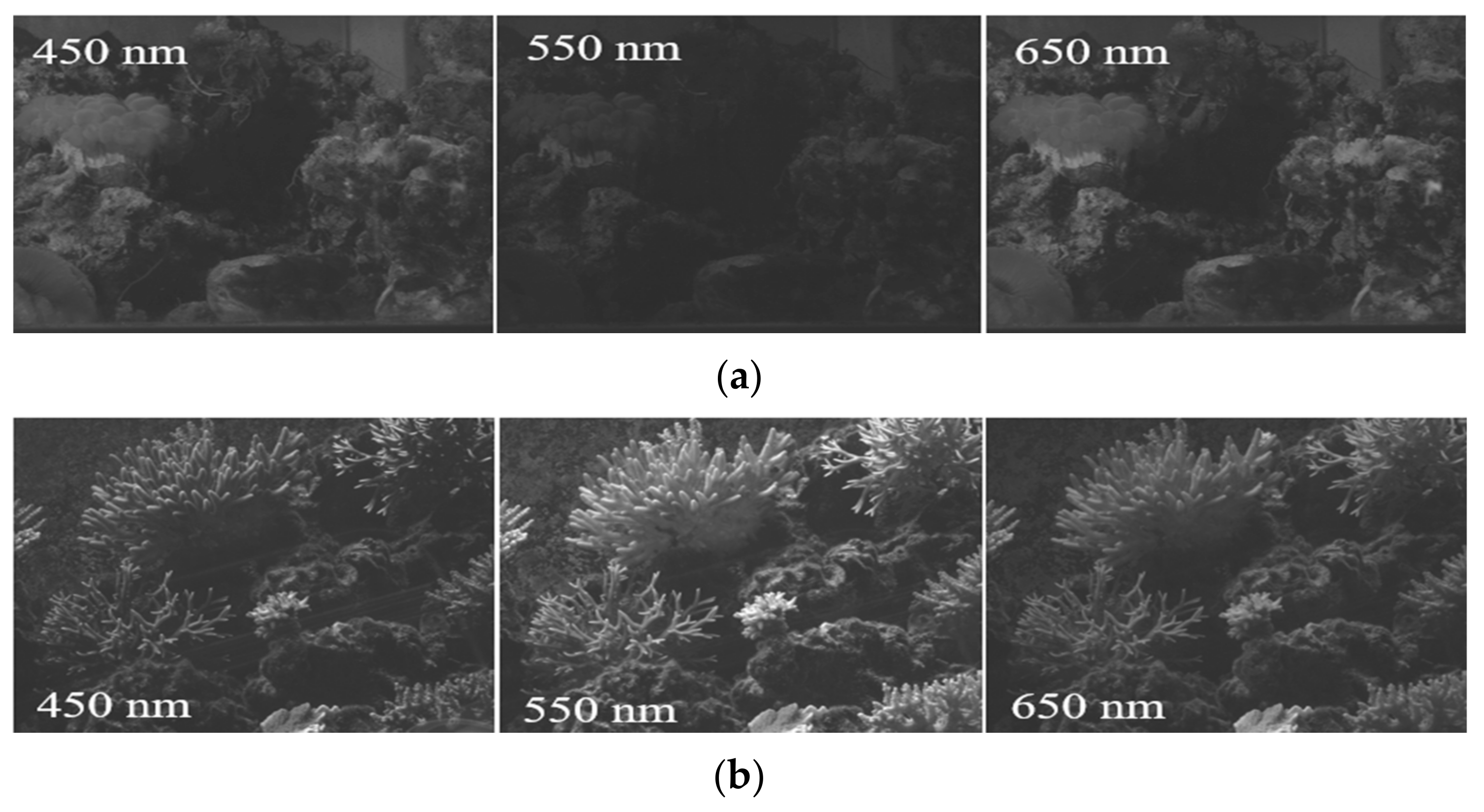
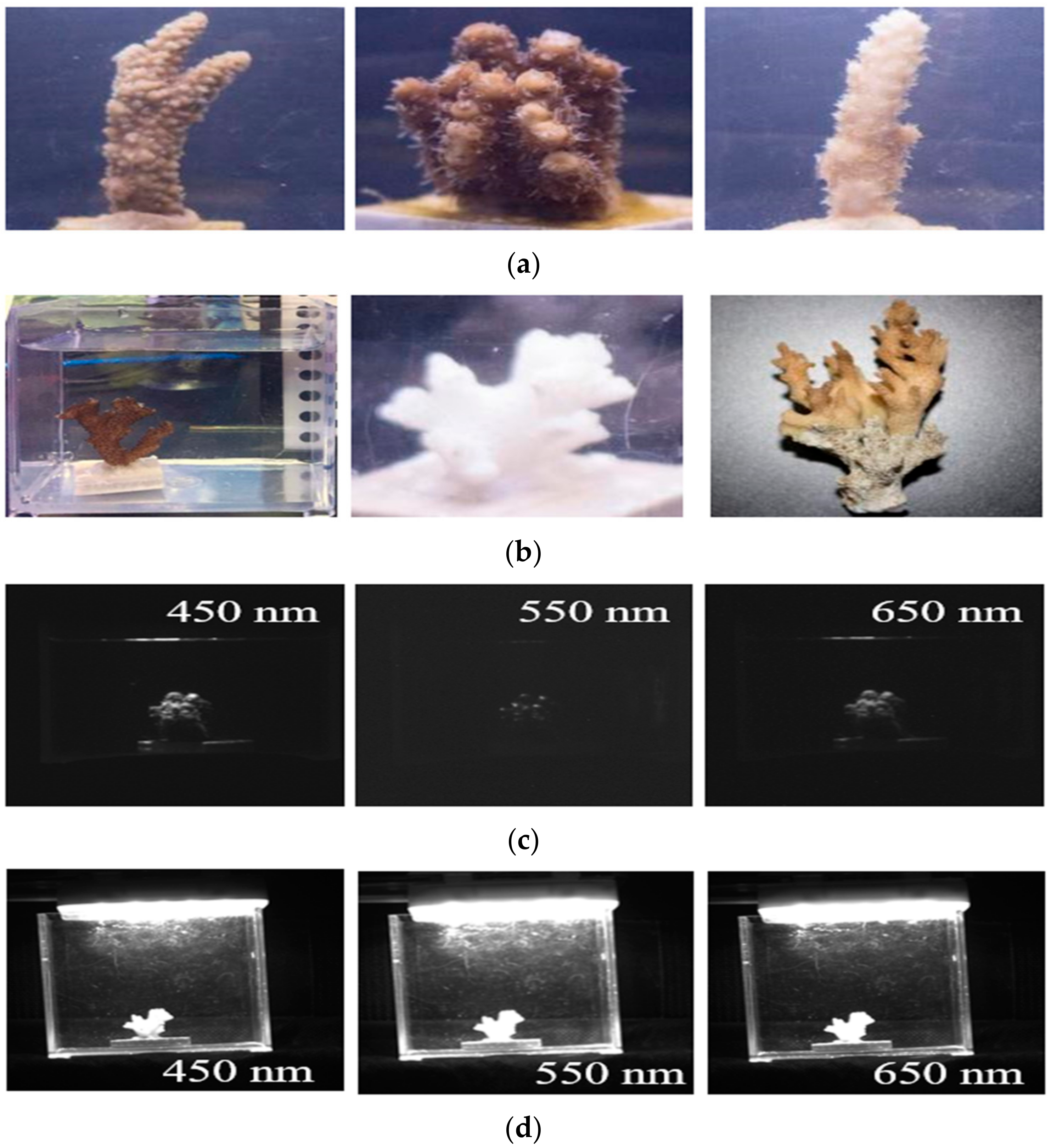
| Third Institute of Oceanography, MNR, Fujian, Xiamen. | Plerogyra sinuosa, Acropora sp. | Figure A1 |
| Institute of Deep-sea Science and Engineering, Chinese Academy of Sciences, Hainan, Sanya. | Dead coral skeleton, Acropora sp. | Figure A2 |
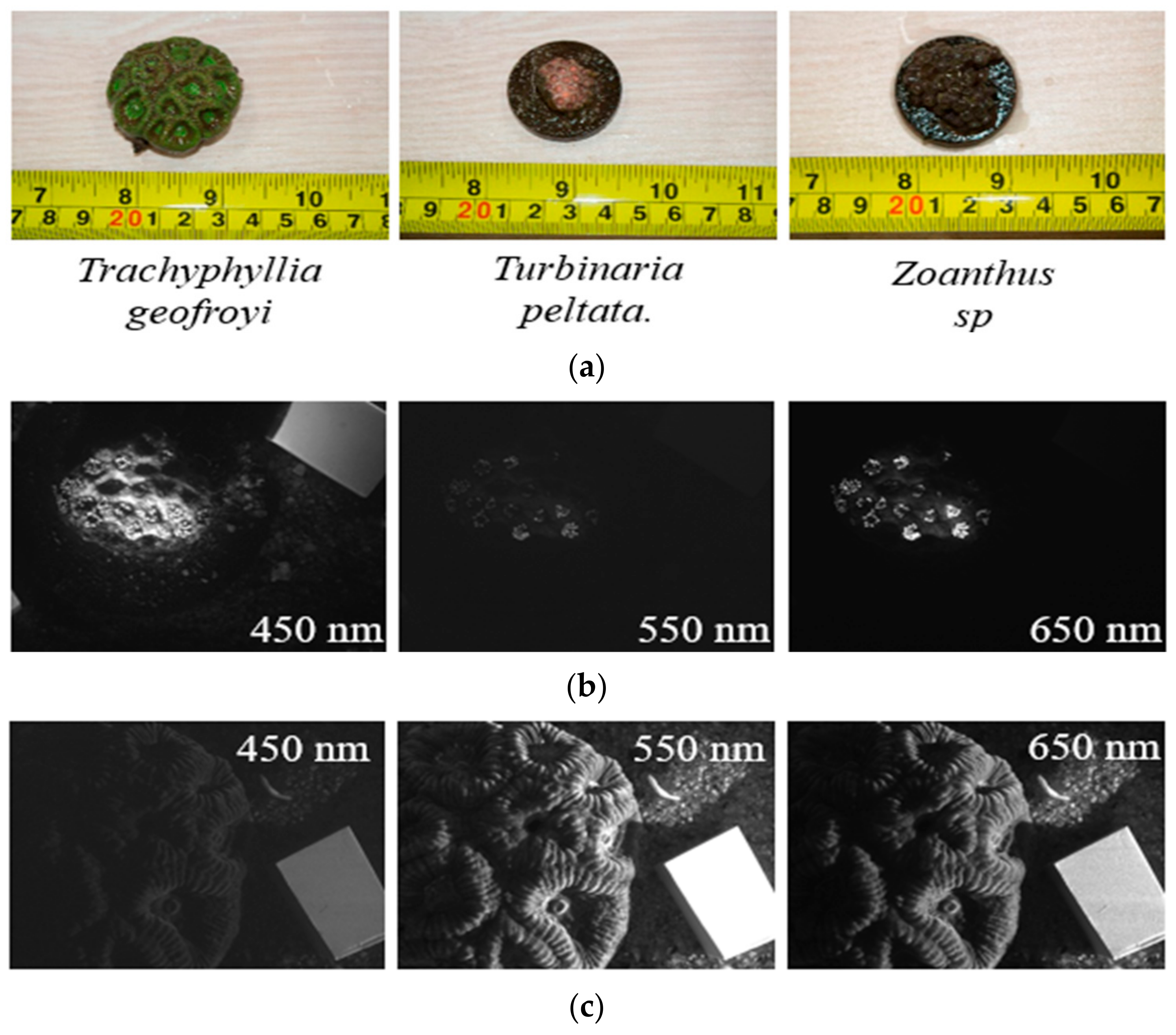
| Ocean Optics Laboratory of Zhejiang University, Zhejiang, Zhoushan. | Trachyphyllia Geofroyi, Turbinaria peltate, Zoanthus sp. | Figure A3 |
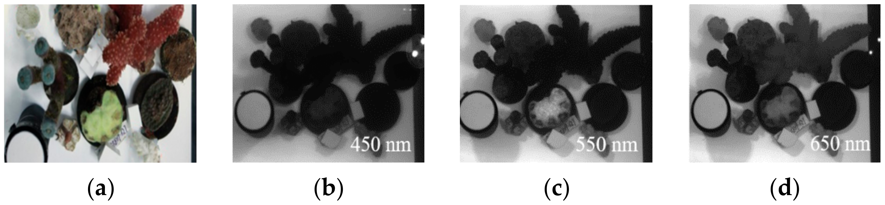
| Ocean Optics Laboratory of Zhejiang University, Zhejiang, Zhoushan. | Dead coral skeleton, Montipora Capricornis, Trachyphyllia Geofroyi, Montipora digitate, Caulastrea furcate, Hydnophora exesa, Nephthyigorgia sp. | Figure A4 |
| Shenzhen Da’ao Bay, Coral conservation base about 8 m depth. 22°33′47″ N and 114°27′37″ E | Mainly Acropora sp. | Figure A5 and Figure A6 |
| Spectral Images | RGB Images | RGB Images from Web Crawler | Total | |
|---|---|---|---|---|
| Positive sample | 144 | 2128 | 400 | 2672 |
| Negative sample | 150 | 1209 | 100 | 1459 |
| Total | 294 | 3337 | 500 | 4131 |
| Training Set 90% | Validation Set 10% | Total | |
|---|---|---|---|
| Single channel RGB image | 10,359 | 1152 | 11,511 |
| Spectral image | 174 | 20 | 194 |
| Total | 10,533 | 1172 | 11,705 |
| Training Set 90% | Validation Set 10% | Total | |
|---|---|---|---|
| Single channel RGB image | 1552 | 176 | 1728 |
| Spectral image | 1369 | 153 | 1522 |
| Total | 2921 | 329 | 3250 |
Publisher’s Note: MDPI stays neutral with regard to jurisdictional claims in published maps and institutional affiliations. |
© 2021 by the authors. Licensee MDPI, Basel, Switzerland. This article is an open access article distributed under the terms and conditions of the Creative Commons Attribution (CC BY) license (http://creativecommons.org/licenses/by/4.0/).
Share and Cite
Song, H.; Mehdi, S.R.; Zhang, Y.; Shentu, Y.; Wan, Q.; Wang, W.; Raza, K.; Huang, H. Development of Coral Investigation System Based on Semantic Segmentation of Single-Channel Images. Sensors 2021, 21, 1848. https://doi.org/10.3390/s21051848
Song H, Mehdi SR, Zhang Y, Shentu Y, Wan Q, Wang W, Raza K, Huang H. Development of Coral Investigation System Based on Semantic Segmentation of Single-Channel Images. Sensors. 2021; 21(5):1848. https://doi.org/10.3390/s21051848
Chicago/Turabian StyleSong, Hong, Syed Raza Mehdi, Yangfan Zhang, Yichun Shentu, Qixin Wan, Wenxin Wang, Kazim Raza, and Hui Huang. 2021. "Development of Coral Investigation System Based on Semantic Segmentation of Single-Channel Images" Sensors 21, no. 5: 1848. https://doi.org/10.3390/s21051848
APA StyleSong, H., Mehdi, S. R., Zhang, Y., Shentu, Y., Wan, Q., Wang, W., Raza, K., & Huang, H. (2021). Development of Coral Investigation System Based on Semantic Segmentation of Single-Channel Images. Sensors, 21(5), 1848. https://doi.org/10.3390/s21051848