Article

Artificial Neural Networks, Sequence-to-Sequence LSTMs, and Exogenous Variables as Analytical Tools for NO2 (Air Pollution) Forecasting: A Case Study in the Bay of Algeciras (Spain)

by
Javier González-Enrique
1,*,
Juan Jesús Ruiz-Aguilar
2,
José Antonio Moscoso-López
2,
Daniel Urda
3,
Lipika Deka
4 and
Ignacio J. Turias
1
1
Intelligent Modelling of Systems Research Group (MIS), Department of Computer Science Engineering, Polytechnic School of Engineering, University of Cádiz, 11204 Algeciras, Spain
2
Intelligent Modelling of Systems Research Group (MIS), Department of Industrial and Civil Engineering, Polytechnic School of Engineering, University of Cádiz, 11204 Algeciras, Spain
3
Grupo de Inteligencia Computacional Aplicada (GICAP), Departamento de Ingeniería Informática, Escuela Politécnica Superior, Universidad de Burgos, Av. Cantabria s/n, 09006 Burgos, Spain
4
The De Montfort University Interdisciplinary Group in Intelligent Transport Systems (DIGITS), Department of Computer Science and Informatics, De Montfort University, Leicester LE1 9BH, UK
*
Author to whom correspondence should be addressed.
Sensors 2021, 21(5), 1770; https://doi.org/10.3390/s21051770
Submission received: 11 February 2021 / Revised: 22 February 2021 / Accepted: 28 February 2021 / Published: 4 March 2021

Abstract

:
This study aims to produce accurate predictions of the NO2 concentrations at a specific station of a monitoring network located in the Bay of Algeciras (Spain). Artificial neural networks (ANNs) and sequence-to-sequence long short-term memory networks (LSTMs) were used to create the forecasting models. Additionally, a new prediction method was proposed combining LSTMs using a rolling window scheme with a cross-validation procedure for time series (LSTM-CVT). Two different strategies were followed regarding the input variables: using NO2 from the station or employing NO2 and other pollutants data from any station of the network plus meteorological variables. The ANN and LSTM-CVT exogenous models used lagged datasets of different window sizes. Several feature ranking methods were used to select the top lagged variables and include them in the final exogenous datasets. Prediction horizons of t + 1, t + 4 and t + 8 were employed. The exogenous variables inclusion enhanced the model’s performance, especially for t + 4 (ρ ≈ 0.68 to ρ ≈ 0.74) and t + 8 (ρ ≈ 0.59 to ρ ≈ 0.66). The proposed LSTM-CVT method delivered promising results as the best performing models per prediction horizon employed this new methodology. Additionally, per each parameter combination, it obtained lower error values than ANNs in 85% of the cases.

1. Introduction

Nowadays, air pollution represents one of the main problems that affect the population’s quality of living, especially in densely populated areas. Low air quality can produce very harmful effects on human health, particularly on children and senior citizens [1,2]. Additionally, it also generates a sizable economic impact due to the increase in the cost of healthcare services.
Among air pollutants, nitrogen dioxide (NO2) generates a great deal of concern as it is considered a critical factor for air quality demise in urban areas [3]. This toxic gas is highly corrosive, very reactive, and possesses an intense irritating capacity [4]. NO2 origins are manifold: it is linked with traffic emissions and industrial operations, including combustion processes [5]. However, it is mainly a secondary pollutant, and its primary source can be found in the oxidation reactions between nitrogen oxides (NO) and ozone (O3) in the atmosphere [6]. The adverse effects of exposure to nitrogen dioxide include several diseases, such as bronchitis or pneumonia [7]. Its long-term impact on mortality is as remarkable as the effect produced by particulate matter [8]. Additionally, it has a significant role in generating photochemical smog acid rain [9].
Considering all the harmful effects that nitrogen dioxide may produce, it becomes essential to create accurate models to determine its future concentrations. Previous studies have addressed this purpose using two main approaches: deterministic approaches and statistical prediction. The deterministic approach employs mathematical formulations and the simulation of various physical and chemical processes, such as emission models, to predict airborne pollutants [10,11]. On the other hand, the statistical prediction approach creates statistical models based on historical data [12]. Unlike deterministic models, statistical techniques are not based on understanding the processes that regulate the change mechanism of pollutant concentrations. They are centered on discovering relations among historical data. Once found, these correlations are applied to the forecasting of future pollution levels. This statistical approach has been recognized as a viable alternative to the deterministic methods and, according to Catalano and Galatioto [13], can deliver better-performing models in short-term air pollutant concentrations. However, statistical methods are based on the assumption that the relations between variables are linear [14]. The irruption of machine learning (ML) techniques made possible the creation of models that could detect and capture non-linear relationships between variables. As a result, ML methods have been widely adopted by researchers for air quality prediction.
Several works devoted to NO2 time series forecasting using ML models can be found in the scientific literature in the last two decades. We can cite the work of Gardner and Dorling [15], who addressed the modeling of hourly NO2 concentrations using artificial neural networks (ANNs) in conjunction with meteorological data. Their results revealed how the proposed approach outperformed regression-based models. Another interesting study was undertaken by Kolehmainen et al. [16], where ANNs were employed to predict NO2 concentrations in Stockholm (Sweden). The authors obtained remarkable results using average NO2 values and several meteorological variables to feed the models. Viotti et al. [17] used ANNs for short and middle long-term forecasting of several pollutants, including NO2. Models exhibited excellent performances with a 1-h ahead prediction horizon. As the prediction horizon increased, the model’s performance decreased but was still better than deterministic models. Kukkonen et al. [18] evaluated the ANN model’s performance compared to other linear and deterministic models. Results brought to light how the neural network models provided better performances than the rest of the techniques tested. Aguirre-Basurko et al. [19] predicted O3 and NO2 in Bilbao (Spain). The authors compared ANN and multiple linear regression models using traffic data and meteorological variables as exogenous inputs in their study. Models were tested in several prediction horizons from t + 1 to t + 8, and ANN models showed the best performances in nearly all the proposed cases. Kumar and Jain [20] utilized an autoregressive moving average (ARIMA) approach to forecasting O3, NO, NO2, and CO with satisfactory results. Rahman et al. [21] compared ARIMA, fuzzy logic models, and ANN models to forecast the Air Pollution Index (API) in Malaysia. The API prediction implies predicting five pollutant concentrations: PM10, O3, CO2, SO2, and NO2. Results showed how ANN models gave the smallest forecasting errors. Bai et al. [22] utilized ANNs in conjunction with wavelet decomposition techniques to predict several pollutants, including NO2. The prediction horizon was set to 24 h, and results showed how the combined approach produced better results than standard ANNs. Finally, Van Roode et al. [23] proposed a hybrid model to forecast the NO2 concentration values with a one-hour prediction horizon in the Bay of Algeciras area (Spain). The authors employed LASSO to predict the linear part of the time series and ANN models to predict the residuals in a two-stage approach. The results confirmed that the proposed hybrid approach presented better performances than any of the particular methods employed.
Among machine learning methods, deep learning (DL) techniques have gained tremendous popularity in recent years. DL uses denser artificial neural networks combined with sequential layers and larger datasets than traditional machine learning methods. Long short-term memory networks (LSTMs) are recurrent neural networks specially designed for supervised time series learning [24]. Several studies have employed LSTMs to forecast pollutants in the scientific literature. We can cite the work of Kök et al. [25], where LSTMs and support vector regression (SVR) models were used to predict NO2 and O3 with a t + 1 horizon. Results showed how the LSTM model outperformed the SVR model. Another interesting study was undertaken by Pardo and Malpica [26], who proposed different LSTM models to predict NO2 levels for t + 8, t + 16 and t + 24 prediction horizons in Madrid (Spain). Finally, Rao et al. [27] compared LSTM based recurrent neural networks and SVR applied to air quality prediction. The results showed how the LSTM approach obtained better forecasting performances than the remaining method employed for all the pollutants considered.
Despite not explicitly being devoted to nitrogen dioxide forecasting, there are two interesting works worth mentioning. Kim et al. [28] developed a system to obtain daily PM10 and PM2.5 predictions in South Korea. In this work, the performances of LSTMs and chemical transport model simulations (more specifically, the Community Multiscale Air Quality (CMAQ) model) were compared. Different meteorological variables and several pollutants data (particulate matter, SO2, NO2 and NO3) were employed as input variables of the LSTM models. Results showed how LSTMs were able to outperform the CMAQ predictions in most of the cases considered. In the case of the study carried out by Carnevale et al. [29], a system to predict air quality in Milan (Italy) was proposed. This study was focused on obtaining up to 2 days ahead PM10 and ozone concentration predictions. A two-stage procedure was followed. In the first stage, neural network predictions were obtained for a monitoring network station located in the study area using exogenous variables. In the second stage, the forecasts obtained at each station were interpolated using the cokriging technique. Additionally, a deterministic chemical transport model was also included as a secondary variable. The proposed methodology provided satisfactory results and constituted a reliable way to give the decision-makers air quality forecasting.
In the present study, ANNs and sequence-to-sequence LSTMs models are developed to forecast NO
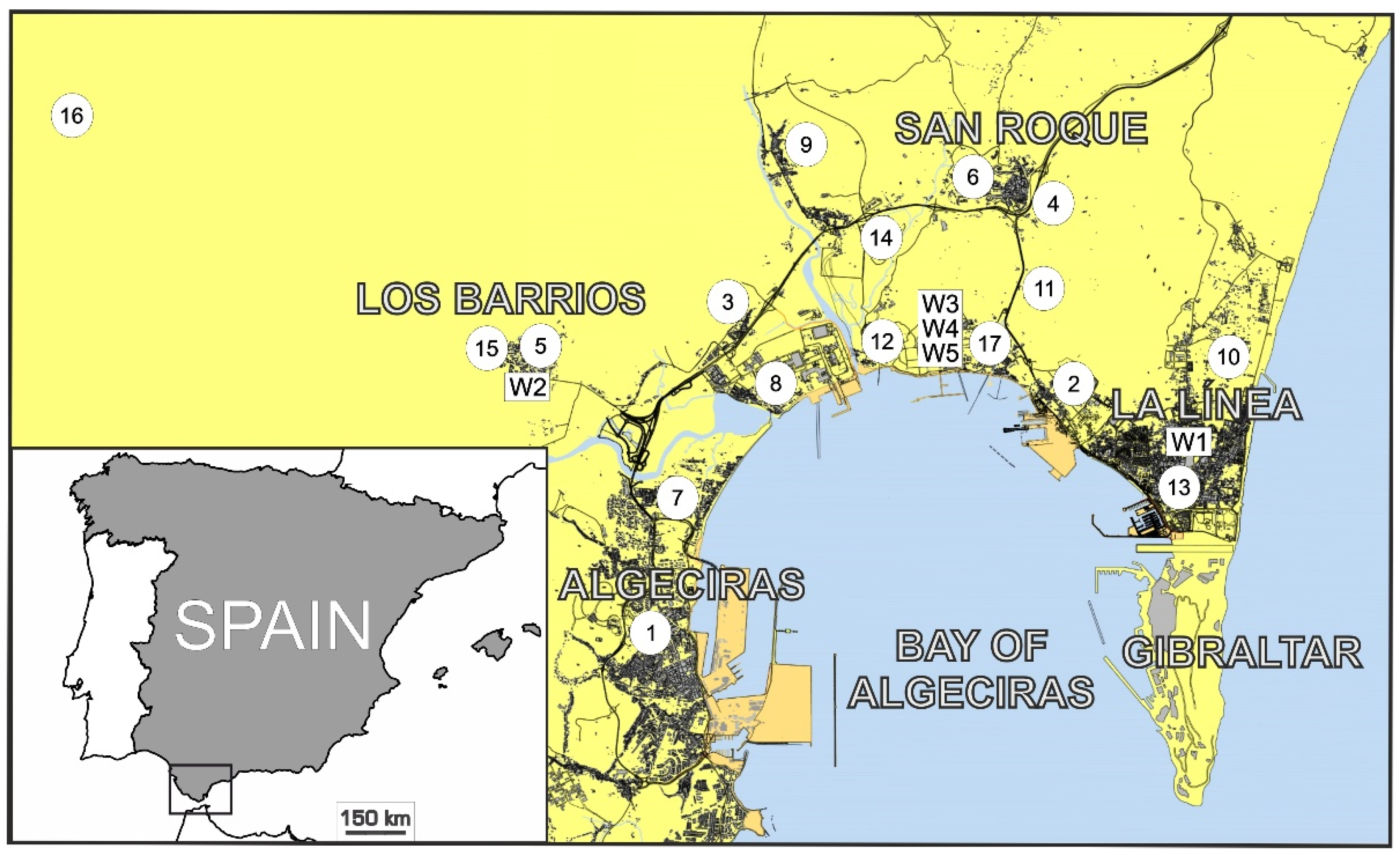
2 concentrations in a specific station of a monitoring network located in the Bay of Algeciras area (Spain). The selected station is located in Algeciras, the study area’s principal city (see Figure 1). The primary goal is to build accurate statistical models to predict NO2 levels with t + 1, t + 4, and t + 8 prediction horizons. Two different approaches were followed to create the forecasting models. Only the NO2 data from the selected station were employed to feed the models in the first approach. In the second approach, exogenous variables were added to the set of predictor variables. In that sense, NO2 data from the network’s remaining stations, data from other pollutants (NOx, SO2, O3) from EPS Algeciras and other stations, and several meteorological variables were included (see Table 1). Based on the previously mentioned techniques, ANNs, standard sequence-to-sequence LSTMs, and LSTMs using a rolling window scheme in conjunction with a cross-validation procedure for time series (LSTM-CVT) were designed in both approaches. Finally, the obtained results were statistically analyzed and compared to determine the best performing model.
The rest of this paper is organized as follows. Section 2 details the study area and the data used. The modeling methods and feature ranking techniques used in this work are depicted in Section 3. Section 4 describes the experimental design. Section 5 discusses the results. Finally, the conclusions are presented in Section 6.

2. Data and Area Description

The Bay of Algeciras is a densely populated and heavily industrialized region situated in the south of Spain. The total population of this region in 2020 is estimated at 300,000 inhabitants [30]. It contains an oil refinery, a coal-fired power plant, a large petrochemical industry cluster, and one of the leading stainless-steel factories in Europe.
As stated in the Introduction section, this work aims to predict the NO2 concentration levels with different time horizons in a monitoring network’s specific monitoring station. This station is EPS Algeciras (see Figure 1). It is located in Algeciras, the study area’s most populous city. With more than 120,000 inhabitants, its air quality is severely affected by the neighboring industries’ pollutant emissions. Additionally, the Port of Algeciras Bay can be found between the top 5 ship-trading ports in Europe. The high number of import and export operations held in this port implies high numbers of heavy vehicles and vessels every year. Combustion processes related to industrial activities and dense traffic episodes favor NO2 emissions, producing a very complicated pollution scenario (15 × 15 km2).
As was previously indicated, NO2 is one of the main factors of air quality decrease in urban areas. Therefore, having accurate models to predict its forthcoming concentrations becomes a critical task for environmental and governmental agencies. The proposed models can constitute a useful set of tools to predict exceedance episodes and take the corresponding corrective measures to avoid them. Additionally, the techniques presented in this article can also be applied to improve other pollutants’ predictions. These improved values can also help enhance the Air Quality Index’s [31] forecasts for the area of study.
The data used in this work was measured by an air monitoring network deployed in the Bay of Algeciras area. It contains 17 monitoring stations and five weather stations. These weather stations are located in Los Barrios (W1), La Línea (W2), and a refinery property of the CEPSA company in different heights (W3 at 10 m, W4 at 60 m, and W5 at 15 m). Figure 1 shows the position of the stations in the study area.
The database contains records of NO2, NOx, SO2, and O3 average hourly concentrations from January 2010 to October 2015. Several meteorological variables, measured hourly at the mentioned weather stations for the same period, are also included. The Andalusian Environmental Agency kindly provided all these measures. The complete list of variables included in the database is shown in Table 1.
Table 2 details the correspondence between the codes used in Figure 1 and the monitoring and weather stations. In this table, the pollutants and meteorological variables measured at each station are also indicated. It is important to note that not all pollutants are measured in all the monitoring stations.
The database was preprocessed to eliminate possible outlier values and inaccurate measures caused by instrumental errors. After that, a process to impute this database’s missing values was applied using artificial neural networks as the estimation method.

3. Methods

Different models have been created to predict the NO2 level concentrations in this study. Two main forecasting techniques were employed: artificial neural networks and sequence-to-sequence LSTMs. Additionally, a new methodology was proposed based on the LSTM technique previously mentioned: LSTM-CVT. A concise description of these forecasting techniques is presented in Section 3.1.
The input data for ANNs and the input sequence for LSTM-CVT have been obtained using a rolling window method. The procedure to build the new lagged variables dataset is described in Section 3.2. Additionally, the ANN and LSTM-CVT models employ a cross-validation method for time series described in Section 3.3.
As was stated in the Introduction section, two different approaches have been compared in this study according to the type of input variables used. In the second one, the use of exogenous variables implies a group of lagged variables for ANN and LSTM-CVT models equal to the selected window size multiplied by the total number of input variables. Section 3.4 describes the feature ranking methods employed in this work to selects the best among these lagged variables.

3.1. Forecasting Techniques

3.1.1. Artificial Neural Networks

Artificial neural networks are a branch of machine learning techniques inspired by how the human brain operates to recognize the underlying relationships in a data set. They are made of several interconnected non-linear processing elements, called neurons. These neurons are arranged in layers, which are linked by connections, called synapses weights. ANNs can detect and determine non-linear relationships between variables. They can act as non-linear functions that map predictors and dependent variables.
Feedforward multilayer perceptron trained by backpropagation (BPNN) [32] is the most commonly used neural network type. Its architecture includes an input layer, one or more hidden layers, and an output layer. The networks are organized in fully connected layers. Their learning process is based on information going forward to the following layers and errors being propagated backward, in a process called backpropagation. According to Hornik et al. [33], feedforward neural networks with a single hidden layer can approach any function if they are correctly trained and contain sufficient hidden neurons. Hence, they are considered a type of universal approximators. BPNNs can be applied either to regression or classification problems [34] where no a priori knowledge is known about the relevance of the input variables. These characteristics make them an adequate method to solve different problems of high complexity, especially non-linear mappings [35]. However, ANNs also present some disadvantages: the inexistence of a standard approach to determine the number of hidden units and possible overfitting affecting the models.
In this work, BPNNs models have been trained using the scaled conjugate gradient backpropagation algorithm [36] to build NO2 forecasting models. The generalization capability of the mentioned models constitutes a crucial matter. Generalization can be defined as the network’s ability to produce good results for unseen new data [34]. Therefore, the reduction of the generalization error becomes essential to obtain accurate prediction models. In that sense, the early stopping technique [35,37] was employed in the models’ training phase to reduce overfitting and avoid generalization issues. The optimal number of hidden neurons was settled by a resampling procedure using 5-fold time-series cross-validation (see Section 3.3). The authors have successfully applied a similar resampling procedure in previous works [38,39,40,41,42], but in this case, it has been modified to time series prediction.

3.1.2. Long Short-Term Memory Networks

Long short-term memory networks are a type of recurrent neural network proposed by Hochreiter and Schmidhuber [43]. Some years later, they were greatly enhanced by Gers et al. [24] by including the fundamental forget gate concept. Standard RNNs can learn past temporal patterns and correlations but are limited when dealing with long-term dependencies in sequences because of the vanishing gradient problem [44,45]. LSTMs overcome this situation by including a special type of unit called memory blocks in their architecture. These units allow LSTMs to decide which meaningful information must be retained, learn long-term dependencies and capture contextual information from data, making them especially suitable for time series prediction [46].
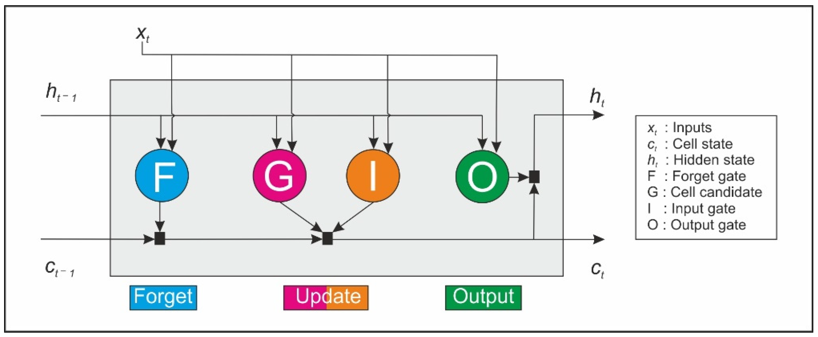
The basic architecture of the LSTM models includes an input layer, a recurrent hidden layer (LSTM layer) containing the memory blocks (also called neurons), and an output layer. One or more self-connected memory cells are included in each memory block. Additionally, three multiplicative units are also contained inside the memory blocks: input, output and forget gates. These gates provide read, write and reset capabilities, respectively, to the memory block. Additionally, they enable LSTMs to decide which meaningful information must be retained and which not relevant information must be discarded. Therefore, they allow the control of information flow and permit the memory cell to store long-term-dependencies. A schematic representation of a memory block with a single cell is shown in Figure 2.
A typical LSTM includes several memory blocks or neurons in the LSTM layer arranged in a chain-like structure. A schematic representation of this structure is depicted in Figure 3.
The cell state and the hidden state are the main properties of this type of network. These properties are sent forward from one memory block to the next one. At time t, the hidden state (ht) represents the LSTM layer’s output for this specific time step. The cell state constitutes the memory that contains the information learning from the previous timestamps. Data can be added or eliminated from this memory employing the gates. The forget gate F controls the connection of the input (xt) and the output of the previous block (hidden state ht−1) with the cell state received from the previous block (ct−1). Then it selects which values from ct−1 must be retained and which ones discarded. After that, the input gate decides which values of the cell state should be updated. The cell candidate then creates a vector of new candidate values, and the cell state is updated, producing ct. Finally, the outputs of the memory block are calculated in the output gate. All this process can be formulated as described in Equations (1)–(5) [47].
i t = δ ( W x i x t + W h i h t 1 + W c i c t 1 + b i )
f t = δ ( W x f x t + W h f h t 1 + W c f c t 1 + b f ) ,
c t = f t c t 1 + i t tan h ( W x c x t + W h c h t 1 + b c )
o t = δ ( W x o x t + W h o h t 1 + W c o c t + b o )
h t = o t tan h ( c t ) ,
where ft, it and ot indicate the state of the forget gate, the input gate and the output gate at time t, respectively. Additionally, ht refers to the hidden state and ct stands for the cell state. Wxi, Whi, Wci, Wxf, Whf, Wcf, Wxc, Whc, Wxo, Who and Wco, correspond to the trainable parameters. The operator denotes the Hadamard product, and the bias terms are represented bi, bf, bc and bo. Finally, δ corresponds to the sigmoid function and tanh indicates the hyperbolic tangent function, which are expressed in Equations (6) and (7), respectively.
δ ( x ) = ( 1 + e x ) 1
tan h ( x ) = e x e x e x + e x
The function of the memory blocks is similar to the neurons in shallow neural networks. In that sense, in the rest of the paper, these memory blocks are referred to as LSTM neurons.

3.2. Lagged Dataset Creation

The time series were transformed into a dataset suitable for the ANN and LSMT-CVT models using a rolling window approach. Autoregressive window sizes of 24, 48 and 72 h were employed. The lagged dataset creation follows a different procedure depending on the type of input variables used: univariate time series and multivariate time series.
In the first case, only the hourly NO2 measures from the selected station were used. New lagged variables were built based on samples of consecutive observations [48]. Thus, the datasets were defined as D k , w s = { x w s i ,   y k i } i = 1 T where T indicates the number of samples, k is the prediction horizon and ws corresponds to the window size. Each i-th sample (row of the dataset) was defined as an input vector x i = { x i ( t ) , , x i ( t ( w s 1 ) ) } concatenated to its corresponding output value y i = ( t + k ) . These new lagged datasets were split into a subset for training and a second subset for testing. The first one included the first 70% of the records and was used to train the models and determine their hyperparameters. The remaining 30% was used as the test subset. In this sense, the models’ performance was tested using unseen data from this subset.
In the second case, data from exogenous features were also included in the group of initial inputs. These time series were also transformed into new lagged datasets appropriate to feed the models using the same window sizes as the previous case. The following steps summarize this process:
  • For each initial variable vj, lagged variables (column vectors) were built in a similar way to the univariate case: { v j ( t ) , , v j ( t ( w s 1 ) ) }.
  • As a second step, the group of potential input variables Pws was created including all the previously created lagged variables Pws = { ( v 1 ( t ) , , v 1 ( t ( w s 1 ) ) ) , , ( v j ( t ) , , v j ( t ( w s 1 ) ) ) } where j indicates the total number of initial variables (77 variables, see Table 1).
  • Then, new datasets were created, including the potential group of variables and the output variable. These datasets were split into training (first 70% records) and test subsets (ending 30% records).
  • As a next step, several feature ranking methods were applied to the elements of Pws in the training subset. The feature ranking methods applied were: mutual information, mutual information using the minimum-redundancy-maximum-relevance algorithm, Spearman’s rank correlation, a modified version of the previously mentioned algorithm using Spearman’s rank correlation, and maximal information coefficient (see Section 3.4). The objective was to select the most relevant among the lagged variable concerning the output variable y = ( t + k ) . The selected lagged variables of the training set were included in the S T r a i n k , w s , f r , p e r set, where fr indicates the feature ranking method applied and per corresponds to the percentage of lagged features selected. Thus, only a small portion of the potential lagged variables was chosen to be finally included as a column in the dataset (the top 5%, top 10% and top 15% variables). Once the ranking and selection process was completed, the same selection criteria were applied to the test set, obtaining the S T e s t k , w s , f r , p e r set.
As the final step, the final training and test datasets were defined as D T r a i n k , w s , f r , p e r = { S T r a i n k , w s , f r , p e r i ,   y k i } i = 1 T and D T e s t k , w s , f r , p e r = { S T e s t k , w s , f r , p e r i ,   y k i } i = 1 T . Each i-th sample (row) of these datasets was defined as an input vector which included the selected lagged variables, as well as its corresponding output value y i = ( t + k ) . Consequently, the datasets included the selected lagged variables in separate columns and the output variable y occupying the final column.

3.3. Time Series Cross-Validation

Cross-validation is a widespread technique in machine learning. However, as was stated by Bergmeir and Benítez [49], there exist some problems regarding dependencies and temporal evolutionary effects within the time-series data. Traditional cross-validation methods do not adequately address these issues. In the k-fold cross-validation method [50,51], all the available training data is randomly divided into k folds. The training procedure is then performed using k − 1, folds, and the error is obtained using the remaining fold as the test set. This procedure is repeated k times so that each fold is used as the test set once. Finally, the error estimate is obtained as the average error rate on test examples.
Bergmeir and Benítez [49] recommend using a blocked cross-validation method for time series forecasting to overcome these shortcomings. This procedure follows the same steps as the k-fold cross-validation method, but data is partitioned into k sequential folds respecting the temporal order. Additionally, dependent values between the training and test sets must be removed. In this sense, an amount of lagged values equal to the window size used is removed from the borders where the training and the test sets meet.
In this work, a 5-fold blocked cross volition method was followed. This method allowed us to determine the hyperparameters of the ANN y LSTM-CVT models (in this last case, in conjunction with the Bayesian optimization technique, see Section 4). A representation of this scheme is presented in Figure 4 [52].

3.4. Feature Ranking Methods

The feature ranking methods employed to select the most meaningful lag variables in the lagged dataset creation are briefly presented in this Section.

3.4.1. Mutual Information

Mutual information (MI) [53] measures the amount of information that one vector contains about a second vector. It can determine the grade of dependency between variables. MI can be defined by Equation (8).
M I ( x , y ) = p ( x , y )   log p ( x , y ) p ( x ) · p ( y )   d x d y ,
where x and y are two continuous random vectors, is their joint probability density and p(x) and p(y) are their marginal probability density. Equation (8) can be reformulated to obtain Equation (11) utilizing entropy (Equation (9)) and conditional entropy (Equation (10)).
H ( x ) = S p ( x ) log p ( x ) d x ,
where S is the set of the random vector with p(x) > 0.
H ( y | x ) = p ( x , y ) log p ( x ) p ( x , y ) d x d y ,
where 0 < H ( y | x ) < H ( x ) .
M I ( x , y ) = H ( y ) H ( y | x ) .
The ITE Toolbox [54] was employed to calculate MI throughout the present manuscript.

3.4.2. Maximal Information Coefficient

Proposed by Reshef et al. [55], the maximal information coefficient (MIC) can reveal linear and non-linear relationships between variables and measure the strength of the relationship between them. Given two vectors, x and y, their MIC can be obtained employing Equation (12) [56].
M I C ( x , y ) = max { M I ( x , y ) / log 2 min { n x , n y } } ,
where MI(x,y) indicates the mutual information between x and y, and nx,ny corresponds to the number of bins dividing x and y. This study’s MIC values were obtained through the Minepy package for Matlab [57].

3.4.3. Spearman’s Rank Correlation Coefficient

Spearman’s rank correlation (SRC) assesses the monotonic relationship’s strength and direction between two variables. This non-parametric measure is calculated operating on the data ranks, with values ranging from [−1,1]. Given two variables x and y, the Spearman’s rank correlation between them can be calculated using Equation (13).
r x , y = i = 1 n { ( x i x ¯ ) · ( y i y ¯ ) } i = 1 n ( x i x ¯ ) 2 · i = 1 n ( y i y ¯ ) 2 .

3.4.4. Minimum-Redundancy-Maximum-Relevance

Minimum-redundancy-maximum relevance (mRMR) [58] is a feature ranking algorithm that penalizes redundant features. This algorithm aims to rank the input variables according to their balance between having maximum relevance with the target variable and minimum redundancy with the remaining features. Relevancies and redundancies are calculated using mutual information. The pseudocode of the mRMR algorithm [59], modified to be used in regression problems, is shown in Algorithm A1 of Appendix A.
In this work, MI, MIC, SRC and mRMR were used to select the most relevant variables when exogenous variables were employed (see Section 3.2). Additionally, the mRMR algorithm was also modified so that Spearman’s rank correlation was used to calculate relevancies and redundancies between variables (mRMR-SRC). Consequently, the relevance term (line 2) and the redundancy term (line 5) of the algorithm were modified, as shown in Algorithm A2 of Appendix A.

4. Experimental Procedure

In this study, ANNs, sequence-to-sequence LSTM and the proposed LSTM-CVT method were used to predict the NO2 concentration levels in the EPS Algeciras monitoring station (see Table 2 and Figure 1). The following prediction horizons were used to create the forecasting models: t + 1, t + 4, and t + 8. Additionally, two different approaches were followed in the model’s creation regarding the initial input data used: using only the NO2 data from the EPS Algeciras station (univariate dataset) or using all the available data (exogenous dataset). This second possibility includes all the 77 variables listed in Table 1 (NO2 and other pollutants (NOx, SO2, O3) from EPS and the remaining stations and several meteorological variables). As was mentioned in Section 2, the database included hourly measures from January 2010 to October 2015. As the first step for both approaches, all the dataset was preprocessed and standardized.
The performance indexes utilized to evaluate the generalization capabilities of the models and their performance were the Pearson’s correlation coefficient (ρ), the mean squared error (MSE), the mean absolute error (MAE) [60] and the index of agreement (d). Lower values of MSE and MAE are associated with more accurate predictions, while higher values of d and ρ indicate higher performance levels of the models. Their corresponding definitions are shown in Equations (14)–(17).
ρ = i = 1 N ( O i O ¯ ) · ( P i P ¯ ) i = 1 N ( O i O ¯ ) 2 · i = 1 N ( P i P ¯ ) 2 ,
M S E = 1 N   i = 1 N ( P i O i ) 2 ,
M A E = 1 N   i = 1 N | P i O i | ,
d = 1 i = 1 N ( P i O i ) 2 i = 1 N ( | ( P i O ¯ | + | O i O ¯ | ) 2 ,
where P indicates the model predicted values and O represents the observed values.
Table 3 summarizes the characteristics of the forecasting models employed in this paper. A detailed description of the experimental procedure followed in each case is presented in the following subsections.

4.1. LSTM-UN and LSTM-EX Models

These models were built using sequence-to-sequence LSTMs. The sequence-to-sequence architecture employs an encoder-decoder structure to transform the inputs by an encoding procedure to a fixed dimensionality vector. This intermediate vector is then decoded to produce the final output sequence [61]. In this technique, minimal assumptions are made on the sequence structure, and the LSTM models map an input sequence of values corresponding to T time steps x = ( x 1 , , x T ) to an output sequence of values y = ( y 1 , , y T ) .
The univariate and exogenous datasets were split into two disjoint training and testing subsets as a first step. The training subset included the first 70% of the records and was used to train the models and determine their hyperparameters. The remaining 30% was used as the test subset. In this sense, the models’ performance was tested using unseen data from this subset.
In the case of the LSTM-UN models, the univariate datasets were used. Input and output sequences were created for the training and test subsets. The output sequences were obtained from their corresponding input sequences with values shifted by k time steps, where k indicates the forecasting horizon (t + 1, t + 4 and t + 8 in this work). After that, the models were trained using the input and output sequences corresponding to the training subset. Bayesian optimization [62,63] was employed to select the optimal learning hyperparameters utilizing the bayesopt MATLAB function with 500 interactions. The root mean square error was the metric employed in this optimization process. The parameters used are shown in Table 4.
The Adam optimizer was employed to train the LSTM models, whose architecture is detailed in Table 5. A dropout layer [64] was added to the standard architecture used in sequence-to-sequence regression problems. This layer aims to prevent overfitting by randomly setting input elements to zero with a given probability.
Then, the training phase’s best network was fed with the input sequence corresponding to the test subset. As a result, the NO2 predicted values were obtained. Finally, performance measures were assessed by comparing the test subset’s output sequence against these forecasted values.
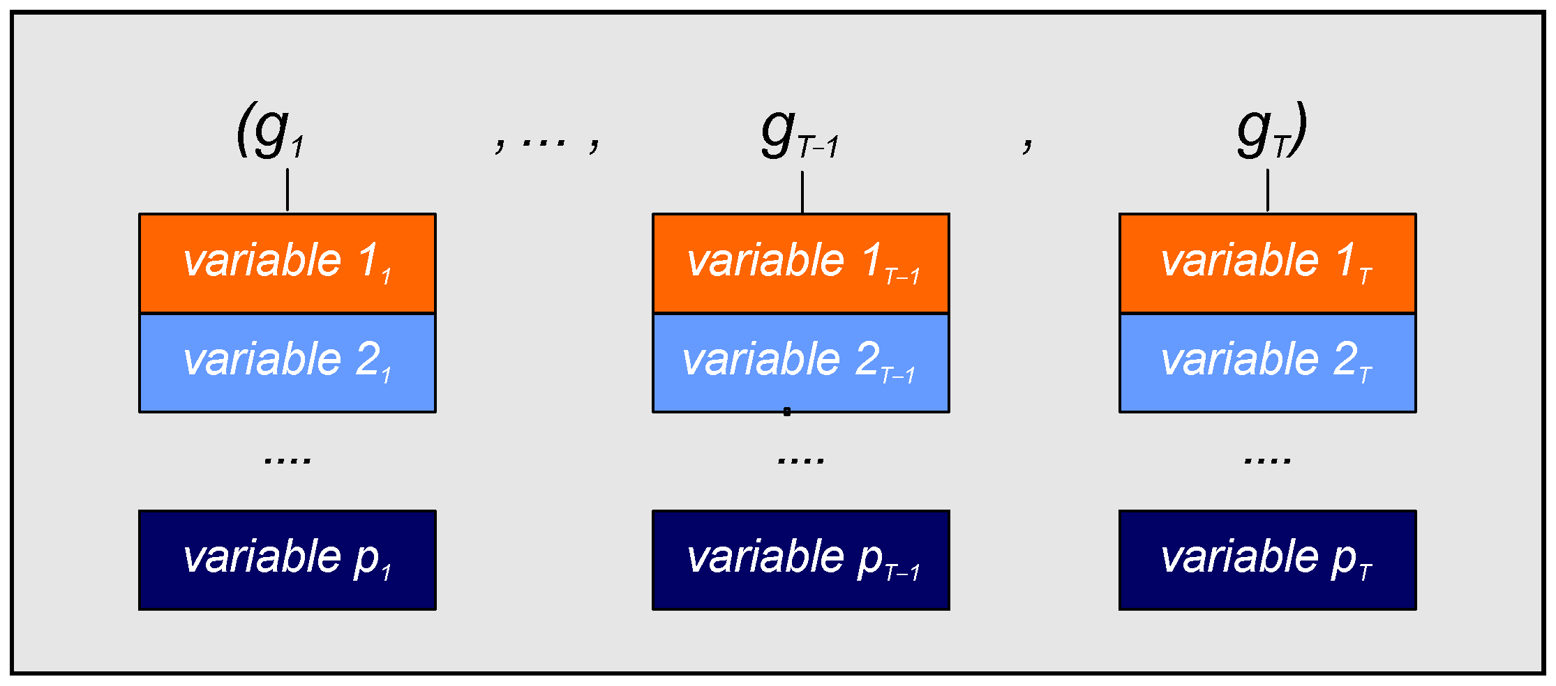
In the case of the LSTM-EX, the process followed is precisely the same as the LSTM-UN models, except for the sequences employed. Thus, the original input sequences corresponding to the training and test subsets had to be modified as these models used the exogenous datasets. Each element of a given original input sequence x was updated to include the new exogenous variables. As a result, an exogenous input sequence g = ( g 1 , , g T ) was obtained. In this new sequence, every element was a column matrix, with g j p x 1 and p corresponding to the total number of variables used (see Table 1). A graphical representation of this exogenous sequence is presented in Figure 5.

4.2. ANN-UN and ANN-EX Models

The NO2 forecasting models using ANNs are illustrated in this subsection. In the first step, lagged training and test datasets were created for each case, as described in Section 3.2. BPNNs were trained using the lagged training dataset following a 5-fold fold cross-validation scheme for time series, as described in Section 3.3. This model’s architecture included a fully connected single hidden layer and several hidden units (1 to 25). The scaled conjugate gradient backpropagation algorithm was employed in conjunction with the early stopping technique. This process was repeated 20 times, and the average results were calculated and stored. Table 6 summarizes all the parameters used in the ANN models.
Additionally, a multi comparison procedure aimed to discover the simplest model without significant statistical differences with the best performing model was undertaken. As a first step, the Friedman test [65] was applied to the test repetitions previously stored. This test (non-parametric alternative to ANOVA) allowed us to determine if relevant differences were present between models built using a different number of hidden units. If differences were detected, models statistically equivalent to the best performing model were found employing the Bonferroni method [66]. Among them, the simplest model was finally selected according to Occam’s razor principle.
After that, a final BPNN model was trained using the entire lagged training dataset. The number of hidden units used was the one determined in the previous step. Once trained, the inputs of the test lagged dataset were used to feed this model. As a result, the NO2 predicted values were obtained, and performance measures were calculated comparing predicted against measured values. This process was repeated 20 times, and the average results were calculated.

4.3. LSTM-CVT-UN and LSTM-CVT-EX Models

The proposed LSTM-CVT method employed sequence-to-sequence LSTMs. However, the input data sequences used did not comprise all the T time steps. In contrast, a rolling window approach was utilized to create lagged training and test datasets, following the procedure described in Section 3.2.
In the case of the LSTM-CVT-UN, the univariate dataset was used to create the lagged training and test datasets. The same parameters (see Table 4) and network architecture (see Table 5) described in the case of the LSTM-UN were also employed in this case. The Adam optimizer was employed in the training process, and 500 interactions were used to determine the optimal hyperparameters through the Bayesian optimization algorithm. The average MSE was the metric employed in this optimization procedure.
Each of these interactions represents a different parameter combination. Per each of them, a 5-fold fold cross-validation scheme for time series (see Section 3.3) was applied to the lagged training dataset. Thus, this dataset was divided into five sequential folds: four of these folds acted as the training subset, while the reaming one served as the test subset. Additionally, an amount of lagged values equal to the window size was eliminated from zones where training and test subsets come together (see Figure 4). Then, the training subset’s input and output sequences were used to train the sequence-to-sequence LSTM models. Once the model was trained, it was fed by the input sequence of the test subset, and the MSE was calculated by comparing the predicted values against the output sequence of the test subset. This procedure was repeated five times until all the folds were employed once as the test subset. Finally, the average value of MSE was calculated.
After the optimal parameters were found, a sequence-to-sequence final LSTM model was trained using the entire lagged training dataset. Once trained, the input sequence of the test lagged dataset was used to feed this model. As a result, the NO2 predicted values were obtained. Performance measures were calculated comparing these values against the output sequence of the test lagged dataset. This process was repeated 20 times, and the average results were calculated.
In the LSTM-EX models, the procedure followed is the same as described in LSTM-UN models. However, as the exogenous datasets were used, the input sequences of their corresponding training and test lagged datasets had to be modified. This modification was performed as described for the LSTM-EX models case (see Section 4.1 and Figure 5).

5. Results and Discussion

This section contains the results obtained in this study on forecasting the NO2 concentration in the EPS Algeciras monitoring station situated in the Bay of Algeciras area. All the calculations were carried out using MATLAB 2020a running on an Intel Xenon 6230 Gold workstation, equipped with 128 GB of RAM and an NVidia Titan RTX graphic card.
The performance metrics depicted in this section correspond to the final models calculated using the test subset with the ending 30% of the database’s records. The models were built employing ANNs, sequence-to-sequence LSTMs and the novel LSTM-CVT method as the forecasting techniques. Prediction horizons of t + 1, t + 4 and t + 8 were established, and their performance was compared in two different scenarios depending on the dataset used (univariate or exogenous datasets, see Section 4).
In the ANN and LSTM-CVT models, different sizes of autoregressive windows were used (24, 48 and 72 h). In the models where an exogenous dataset was used, only the top 5%, 10% or 15% lagged variables were kept (see Section 3.2). This selection was made according to several feature ranking techniques: mutual information, mRMR, Spearman’s rank correlation, mRMR-SRC and MIC (see Section 3.4).
Table 7 shows the average performance for the top models per each prediction horizon. In this table, ws corresponds to the window size, nh is the number of units in the hidden layer (neurons), DP denotes the dropout probability, MBS is the minibatch size, LR corresponds to the learning rate, L2R is the level 2 regularization factor and GD is the gradient decay factor. In the exogenous datasets scenario, the top models per window size are presented. Additionally, Table A1, Table A2, Table A3, Table A4, Table A5 and Table A6 in Appendix A show the results obtained using the univariate dataset and the top models per window size using exogenous datasets. The complete list of models built using exogenous datasets is also presented in Table A7, Table A8 and Table A9 of the mentioned appendix.
A first comparison of the results based on the prediction horizon shows how performance indices worsen as the forecast horizon grows. As further in the future, the prediction goes, the accuracy of the models lowers. Thus, the best performing models go from ρ ≈ 0.90 for t + 1 to ρ ≈ 0.66 for t + 8. A comparison between the top models for each prediction horizon of 
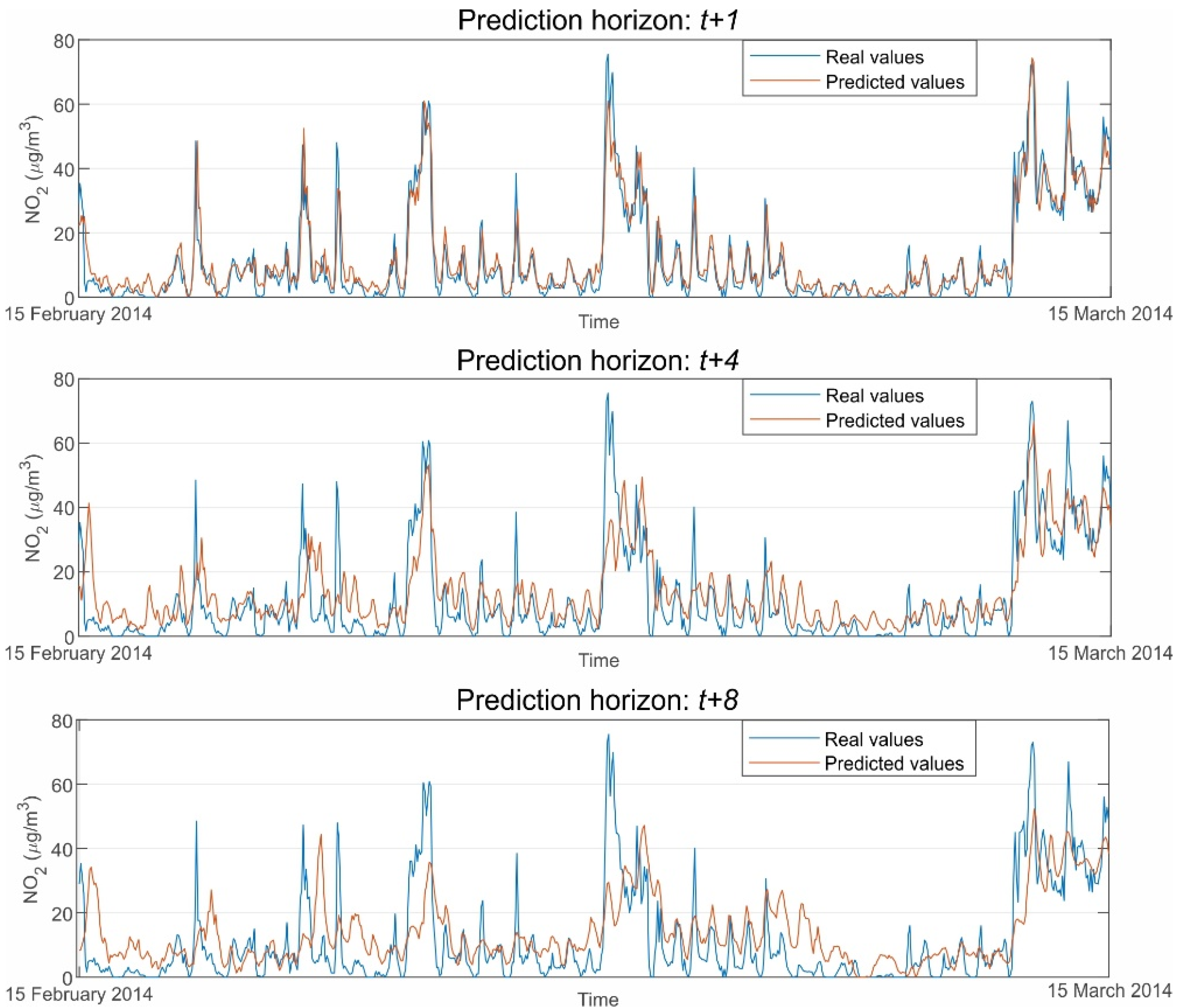
Table 7 is presented in Figure 6. In this figure, observed vs. predicted values of NO2 hourly average concentrations are depicted for the period between the 15 February 2014 and the 15 March 2014.
As can be seen, the fit and adjustment to the measured values are excellent for the best model of the t + 1 prediction horizon. However, the fit’s goodness decreases as the prediction horizons grow, confirming what was previously stated.
Another essential factor in this work is the possible influence of exogenous variables on the models’ performance. In light of the results, exogenous variables’ inclusion boosts the model’s forecasting performance, regardless of the forecasting technique used or the prediction horizon considered. Table 8 shows the perceptual changes in ρ and MSE of the models from Table A1, Table A2, Table A3, Table A4, Table A5 and Table A6 (see Appendix A).
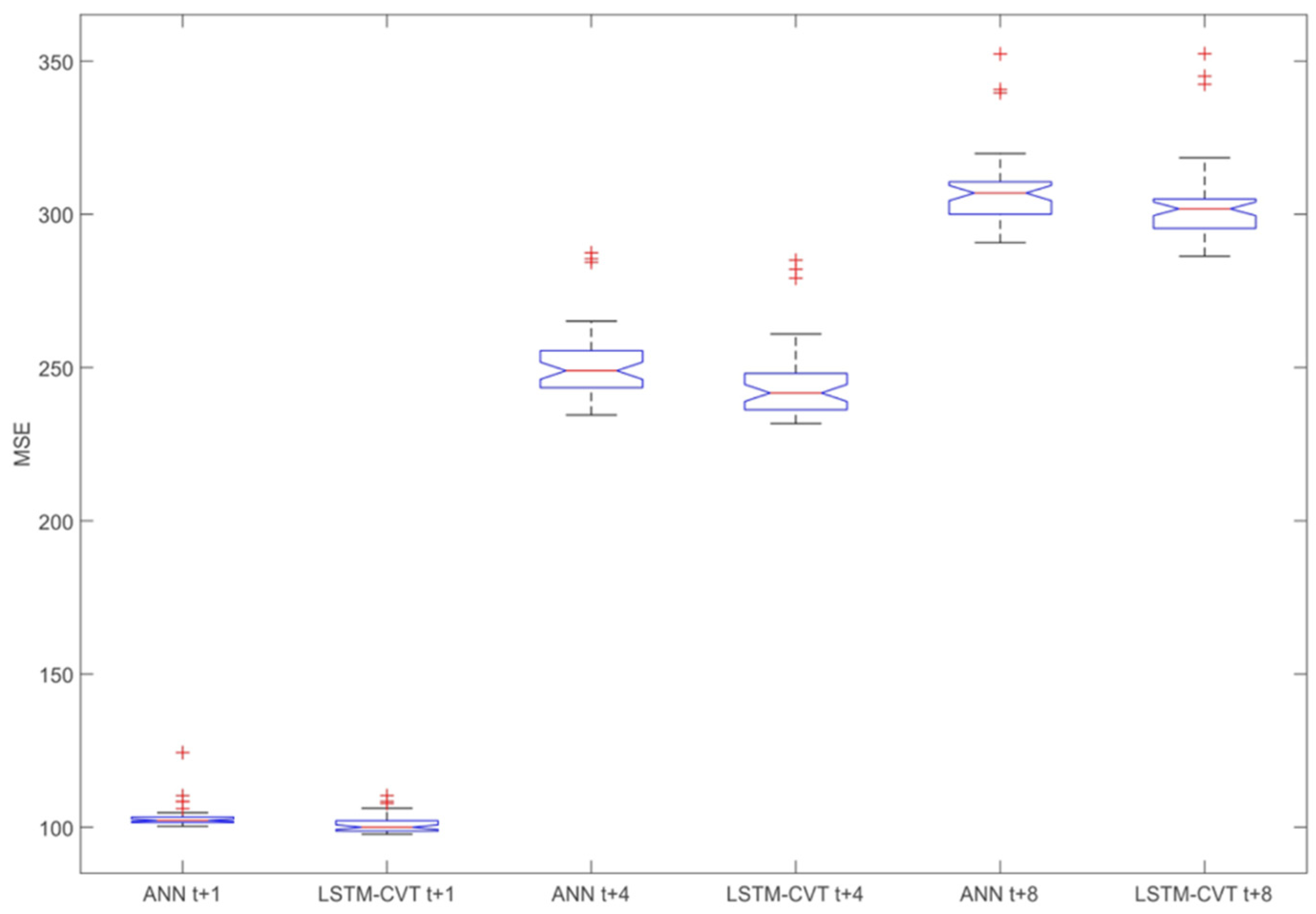
As can be observed, exogenous variables produce a noticeable enhancement in all the cases considered. This improvement becomes greater for t + 4 and t + 8, especially for the Pearson’s correlation coefficient. An in-depth look at the results shows how the proposed LSTM-CVT-EX models lead the prediction horizon scenarios’ performance rankings. Additionally, the LSTM-CVT and ANN best-performing models provide better performance indexes than sequence-to-sequence LSTMs in all the proposed cases. This observation emphasizes the positive effect of the lagged dataset and the time series cross-validation on the LSTM-CVT models, which internally uses sequence-to-sequence LSTMs.
The comparison of the LSTM-CVT and the ANNs models reveals that their performances are much closer than in the previous case. However, all the best performing models per prediction horizon are LSTM-CVT models. This fact can also be observed for each prediction horizon/window size combination presented in Table A1, Table A2, Table A3, Table A4, Table A5 and Table A6. Figure 7 depicts box-plot comparisons of these models for exogenous datasets and t + 1, t + 4 and t + 8 prediction horizons. For each case, their average MSE values have been compared, including all the possible windows size, feature ranking and percentage combinations considered in this work (see Appendix A for the complete list of cases for the exogenous datasets).
Additionally, per each parameter combination (window size + feature ranking method + percentage), ANN and LSTM-VCT models have been compared. The rates of parameter combinations where each technique provides better average MSE values are presented in Figure 8. The representations in Figure 7 and Figure 8 confirm the forecasting capability of the LSTM-CVT method as it offers a lower average MSE than ANN models in the 85% of the total combinations considered.
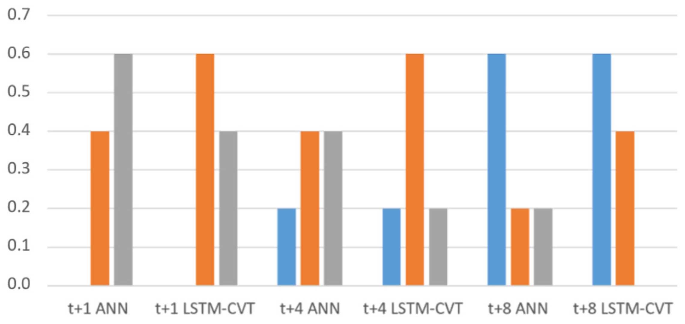
Another interesting aspect is related to the window size, percentage of lagged variables selected used by the top-performing models. Figure 9, Figure 10 and Figure 11 depicts the usage rates of their possible values for these parameters by the top 10% performing models.
As shown in Figure 9, window sizes of 48 h are among the more employed, with an approximate usage of the 43% of the models considered. However, 72 and 24 h are also employed with use percentages of around 30%. The difference is that t + 1 models tend to use larger window sizes (48–72 h), while t + 8 models do the opposite (24 is the preferred window size in this prediction horizon).
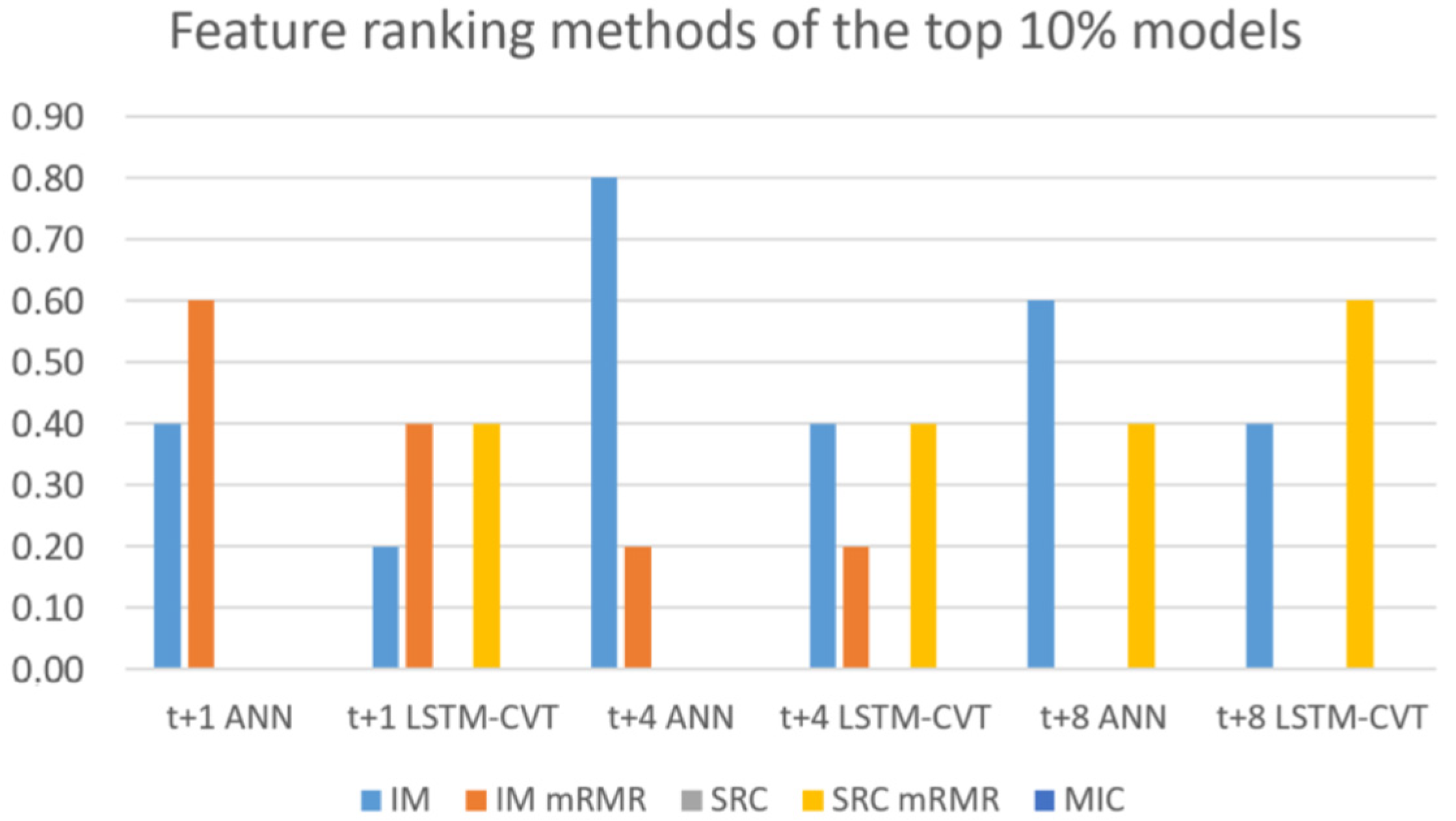
Regarding the feature ranking techniques employed, it is essential to note the influence of these methods in the exogenous lagged dataset creation and, hence, the model’s future performance. Figure 10 shows how the top-performing models only use mutual information, mRMR and mRMR-SRC. In contrast, MIC and standard Spearman’s rank correlation are not employed by these top-performing models. On the one hand, mutual information is applied by around 50% of the models. A closed look to Figure 10 reveals that MI is especially significant in ANN models, while LSTM-CVT models use mRMR-SRC much more. Additionally, the use of mRMR decreases as the prediction horizon grows (it is not employed by any of the top-performing models in t + 8).
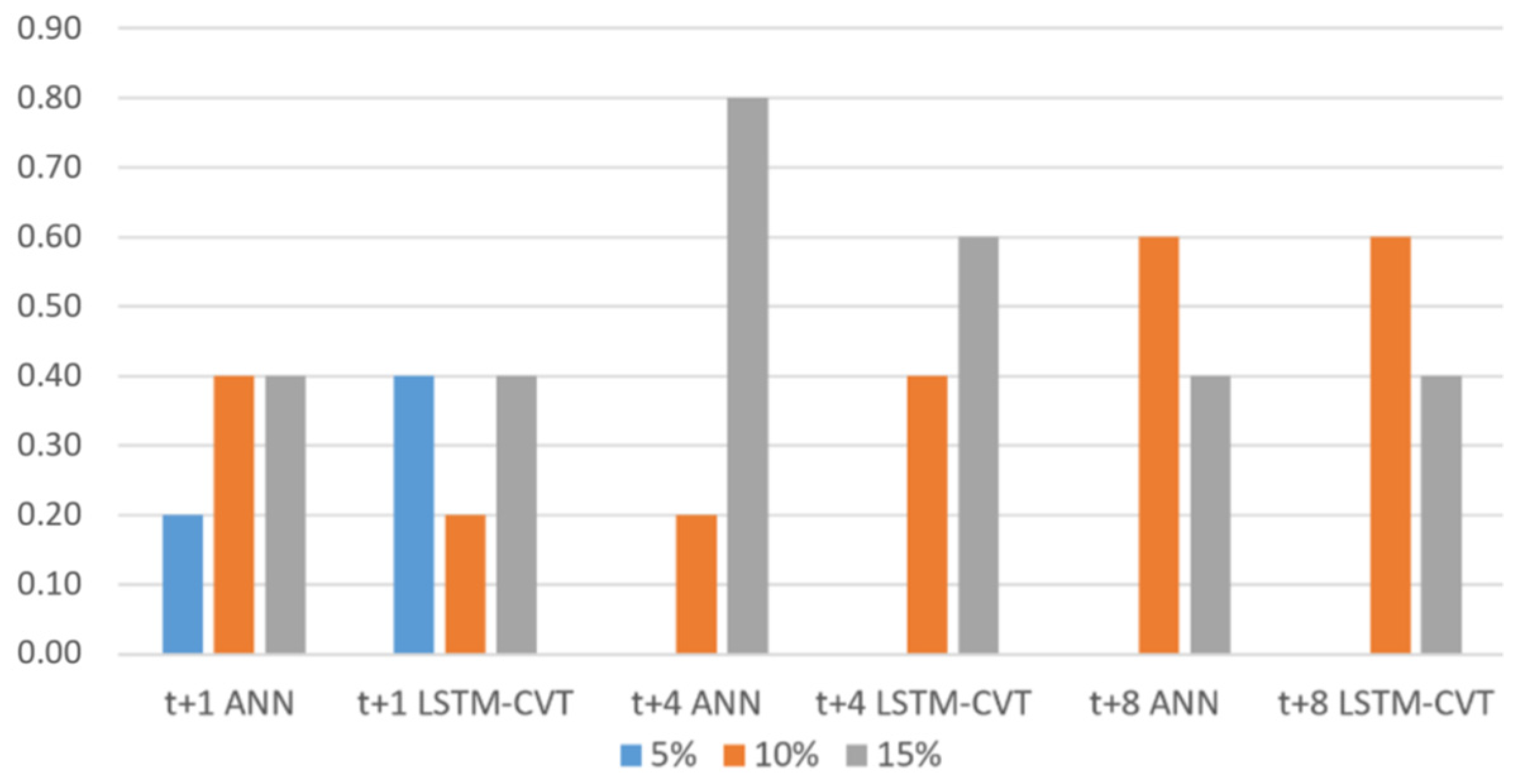
Concerning the percentage of lagged variables used presented in Figure 11, the options of 15% and 10% are used in all the cases. Their use is especially remarkable in longer time horizons. Conversely, the 5% option is only used by t + 1 models that do not need as much information as t + 4 or t + 8 models to provide good forecasting results.

6. Conclusions

This paper aims to produce accurate forecasting models to predict the NO2 concentration levels at the EPS Algeciras monitoring station in the Bay of Algeciras area, Spain. The forecasting techniques employed include ANNs, LSTMs and the newly proposed LSTM-CVT method. This method merges sequence-to-sequence LSTMs with a time-series cross-validation procedure and a rolling window approach to utilize lagged datasets. Additionally, a methodology used to feed standard sequence-to-sequence LSTMs with exogenous variables was also presented. Bayesian optimization was employed to automatically determine the optimal hyperparameters of the LSTM models, including LSTM-CVT.
Three different prediction horizons (t + 1, t + 4 and t + 8) were established to test the forecasting capabilities. Additionally, two different approaches were followed regarding the input data. On the one hand, the first option used a univariate dataset with just the hourly NO2 data measured at the EPS Algeciras monitoring station. On the other hand, the second approach added exogenous features, including NO2 data from different monitoring stations, other pollutants (SO2, NOx and O3) from EPS and the remaining stations, and several meteorological variables.
The procedure used to create the ANN and LSTM-CVT exogenous models includes creating lagged datasets with different window sizes (24, 48 and 72 h). The high number of features employed made it unfeasible to use all the lagged variables produced. Hence, several feature ranking methods were presented and used to select the top 5%, 10% and 15% lagged variables into the final exogenous datasets. Consequently, 45 window size/feature ranking/percentage combinations were arranged and tested per each prediction horizon (see Appendix A).
Exogenous datasets produced a noticeable enhancement in the model’s performance, especially for t + 4 (ρ ≈ 0.68 to ρ ≈ 0.74) and t + 8 (ρ ≈ 0.59 to ρ ≈ 0.66). In the case of the t + 1 horizon, results were closer (ρ ≈ 0.89 to ρ ≈ 0.90). These improvements are found no matter the prediction technique used (see Table A1, Table A2, Table A3, Table A4, Table A5 and Table A6 in Appendix A and Table 8). Despite the noticeable gains in the LSTM model’s performance due to exogenous features, the ANN and LSTM-CVT models’ overachieved all the sequence-to-sequence LSTM models.
The proposed LSTM-CVT method produced promising results as all the best performing models per prediction horizon employed this new methodology. This tendency can also be observed for each prediction horizon/window size combination presented in Table A1, Table A2, Table A3, Table A4, Table A5 and Table A6. Per each parameter combination (window size + feature ranking method + percentage), the performances of this new methodology and ANNs were compared. Results showed how the LSTM-CVT models delivered a lower average MSE than the ANN models in 85% of the total combinations considered. Additionally, models using this methodology performed better than sequence-to-sequence LSTMs models, especially for the t + 4 (ρ ≈ 0.70 against ρ ≈ 0.74) and t + 8 (ρ ≈ 0.63 against ρ ≈ 0.66) prediction horizons.
The percentages of lagged features selected, the feature ranking to be employed and the optimal window sizes were also discussed. Results reveal that forecasting models using a further prediction horizon need to use more information and more exogenous variables. In contrast, models for a closer prediction horizon only need the time series data and less exogenous features.
As results indicate, the new LSTM-CVT technique could be a valuable alternative to standard LSTMs and ANNs to predict NO2 concentrations. This novel method represents an improvement against all the other methods used, which are among the most representative in NO2 time series forecasting literature. Additionally, it is also important to outline the excellent performance of the exogenous models. In the case of ANN-EX and LSTM-CVT-EX models, a new methodology using feature ranking methods was also proposed to deal with the increasing lagged variables as the window sizes grow. In this approach, the importance of the selection of the more significant lagged features becomes essential. Thus, new feature selection techniques will be tested with LSTM-CVT in future works. Furthermore, it is also necessary to highlight the Bayesian optimization procedure employed to train the sequence-to-sequence LSTM models. According to a set of limits previously established, this procedure allows an automatic search of optimal hyperparameters. As a result, the chances of finding the real optimal hyperparameters are considerably higher than other approaches followed in the scientific literature.
Finally, as stated in previous sections, nitrogen dioxide plays a principal role among air pollutants due to the study area’s inherent characteristics. The proposed models and the new methodologies presented can help to predict exceedance episodes in the NO2 concentrations. They can act as decision-making tools that allow the governmental and environmental agencies to take the necessary measures to avoid the possible harmful effects and the associated air quality demise. Additionally, these new methodologies can be applied to other pollutants forecasting and help obtain better AQI predictions in the study area.

Author Contributions

Conceptualization, J.G.-E. and I.J.T.; data curation, J.G.-E. and J.J.R.-A.; formal analysis, J.G.-E.; funding acquisition, I.J.T.; investigation, J.G.-E. and J.J.R.-A.; methodology, J.G.-E.; project administration, I.J.T.; resources, J.G.-E., J.A.M.-L., D.U. and L.D.; software, J.G.-E., J.J.R.-A., J.A.M.-L. and D.U.; supervision, J.J.R.-A., J.A.M.-L., D.U., L.D. and I.J.T.; validation, J.G.-E., J.J.R.-A., J.A.M.-L., D.U. and L.D.; visualization, J.G.-E.; writing—original draft, J.G.-E., J.J.R.-A. and J.A.M.-L.; writing—review and editing, J.G.-E., D.U., L.D. and I.J.T. All authors have read and agreed to the published version of the manuscript.

Funding

This research was funded by MICINN (Ministerio de Ciencia e Innovación-Spain), grant number RTI2018-098160-B-I00, and grant “Ayuda para Estancias en Centros de Investigación del Programa de Fomento e Impulso de la actividad Investigadora de la Universidad de Cádiz”.

Institutional Review Board Statement

Not applicable.

Informed Consent Statement

Not applicable.

Data Availability Statement

Not applicable.

Acknowledgments

Monitoring data has been kindly provided by the Environmental Agency of the Andalusian Government. This research has been carried out during the research stay at the DIGITS Research Group of the De Montfort University (United Kingdom).

Conflicts of Interest

The authors declare no conflict of interest.

Appendix A

Additional tables showing the complete list of models built using univariate datasets and the top models per window size and method using exogenous datasets are presented in this appendix (Table A1, Table A2, Table A3, Table A4, Table A5 and Table A6). Additionally, the complete list of models created using the exogenous dataset is shown in Table A7, Table A8 and Table A9. In these tables, ws is the size of the autoregressive window, nh is the number of hidden units, DP is de dropout probability, MBS is the size of the minibatch, LR indicates the learning rate, L2R is the level 2 regularization factor and GD is the gradient decay factor.
Table A1. Results obtained using the univariate dataset and a prediction horizon of t + 1.
Method NamewsρMSEdMAEnhDPMBSLRL2RGD
LSTM UN-0.876117.8600.9307.112210.009160.0400.0010.559
LSTM-CVT-UN240.884110.4850.9356.7755990.57210240.0050.0000.697
LSTM-CVT-UN480.885109.2110.9366.7595520.09710240.0060.0010.543
LSTM-CVT-UN720.886108.7660.9366.7525070.1905120.0010.0000.430
ANN-UN240.884110.9110.9356.75290.0000---
ANN-UN480.884110.0210.9366.74380.0000---
ANN-UN720.885109.6070.9366.74730.0000---
Table A2. Top models per window size and method using exogenous datasets and a prediction horizon of t + 1.
Method NamewsFeature Ranking Method%ρMSEdMAEnhDPMBSLRL2RGD
LSTM EX--00.892111.5760.9316.8391880.22220480.0080.0010.902
LSTM-CVT-EX24mRMR-SRC100.89998.1770.9416.5565350.6555120.0010.0000.813
LSTM-CVT-EX48IM150.89997.7070.9426.5345800.2455120.0020.0010.331
LSTM-CVT-EX72mRMR50.89997.8490.9416.5293170.6105120.0010.0010.771
ANN-EX24mRMR150.895101.3300.9416.6548-----
ANN-EX48mRMR100.895100.3040.9416.6468-----
ANN-EX72mRMR50.896100.5090.9416.6137-----
Table A3. Results obtained using the univariate dataset and a prediction horizon of t + 4.
Method NamewsρMSEdMAEnhDPMBSLRL2RGD
LSTM UN-0.635303.1610.73912.749990.1845120.0480.0000.404
LSTM-CVT-UN240.669279.0610.78011.9045440.65010240.0250.0000.662
LSTM-CVT-UN480.677273.6860.78611.7936440.72410240.0060.0000.481
LSTM-CVT-UN720.679272.4950.78511.8335550.74910240.0030.0010.492
ANN-UN240.663282.9130.77811.89490.0000---
ANN-UN480.673276.2210.78611.75080.0000---
ANN-UN720.675275.4010.78611.77060.0000---
Table A4. Top models per window size and method using exogenous datasets and a prediction horizon of t + 4.
Method NamewsFeature Ranking Method%ρMSEdMAEnhDPMBSLRL2RGD
LSTM EX---0.701281.2310.78811.6471510.38320480.0050.0000.453
LSTM-CVT-EX24IM150.737231.7150.82910.8795070.13310240.0030.0010.947
LSTM-CVT-EX48mRMR150.739233.0060.82911.2624960.9032560.0010.0010.911
LSTM-CVT-EX72mRMR-SRC150.735234.1170.82511.2466240.9411280.0010.0000.665
ANN-EX24IM150.731236.0960.82510.8627-----
ANN-EX48mRMR150.724242.0630.82011.3663-----
ANN-EX72IM100.732234.5200.82710.9456-----
Table A5. Results obtained using the univariate dataset and a prediction horizon of t + 8.
Method NamewsρMSEdMAEnhDPMBSLRL2RGD
LSTM UN-0.558348.8210.68313.953610.06710240.0230.0000.092
LSTM-CVT-UN240.585332.1770.70813.4883080.2895120.0050.0000.468
LSTM-CVT-UN480.588330.7720.70513.6173070.69410240.0020.0010.040
LSTM-CVT-UN720.588331.0650.71013.5667860.00910240.0020.0010.026
ANN-UN240.581334.8760.70413.4535-----
ANN-UN480.587330.9070.71013.4135-----
ANN-UN720.587331.1040.71013.4334-----
Table A6. Top models per window size and method using exogenous datasets and a prediction horizon of t + 8.
Method NamewsFeature Ranking Method%ρMSEdMAEnhDPMBSLRL2RGD
LSTM EX---0.634305.7330.75112.5633710.47220480.0070.0000.920
LSTM-CVT-EX24mRMR-SRC150.659286.3640.76912.6835510.90810240.0020.0010.304
LSTM-CVT-EX48IM100.658286.5860.77012.4657970.05420480.0020.0010.765
LSTM-CVT-EX72IM150.651292.5850.75912.3984290.9202560.0010.0010.614
ANN-EX24mRMR-SRC100.647294.6920.75412.6412-----
ANN-EX48IM100.652290.7730.76312.5306-----
ANN-EX72IM100.651293.3710.75812.4035-----
Table A7. Forecasting models using exogenous datasets and a prediction horizon of t + 1.
Method NamewsFeature Ranking Method%ρMSEdMAEnhDPMBSLRL2RGD
LSTM EX---0.892111.5760.9316.8391880.22220480.0080.0010.902
ANN-EX24IM50.885110.2740.9346.78616-----
ANN-EX24IM100.891104.6450.9386.6897-----
ANN-EX24IM150.893102.9620.9396.6549-----
ANN-EX24mRMR50.894102.2560.9406.5883-----
ANN-EX24mRMR100.895101.6130.9406.6075-----
ANN-EX24mRMR150.895101.3300.9416.6548-----
ANN-EX24MIC50.890106.0480.9376.6791-----
ANN-EX24MIC100.891104.7010.9386.6662-----
ANN-EX24MIC150.893103.3470.9396.6714-----
ANN-EX24SRC50.892104.6050.9386.6652-----
ANN-EX24SRC100.892103.7810.9386.6872-----
ANN-EX24SRC150.893103.3200.9396.6794-----
ANN-EX24mRMR-SRC50.894102.6450.9396.6323-----
ANN-EX24mRMR-SRC100.894102.0410.9396.6769-----
ANN-EX24mRMR-SRC150.895101.5250.9416.6149-----
ANN-EX48IM50.887108.4030.9356.75115-----
ANN-EX48IM100.894102.1730.9396.64312-----
ANN-EX48IM150.894101.5630.9406.6696-----
ANN-EX48mRMR50.895100.9240.9406.6077-----
ANN-EX48mRMR100.895100.3040.9416.6468-----
ANN-EX48mRMR150.895100.6060.9416.66210-----
ANN-EX48MIC50.845124.3450.8987.2322-----
ANN-EX48MIC100.894102.8650.9406.6567-----
ANN-EX48MIC150.893102.6900.9406.7116-----
ANN-EX48SRC50.894102.2370.9396.6328-----
ANN-EX48SRC100.894101.9180.9406.67210-----
ANN-EX48SRC150.894102.0230.9406.7258-----
ANN-EX48mRMR-SRC50.895101.1900.9406.6416-----
ANN-EX48mRMR-SRC100.894101.5610.9406.6535-----
ANN-EX48mRMR-SRC150.894102.1750.9406.6548-----
ANN-EX72IM50.887108.4110.9356.76020-----
ANN-EX72IM100.895100.7360.9416.62310-----
ANN-EX72IM150.895100.8790.9416.64110-----
ANN-EX72mRMR50.896100.5090.9416.6137-----
ANN-EX72mRMR100.895101.3480.9416.7556-----
ANN-EX72mRMR150.893103.0730.9396.9445-----
ANN-EX72MIC50.893103.3870.9396.6806-----
ANN-EX72MIC100.893102.8850.9396.7124-----
ANN-EX72MIC150.893103.1890.9396.8045-----
ANN-EX72SRC50.894102.2670.9396.6608-----
ANN-EX72SRC100.894101.9850.9406.7298-----
ANN-EX72SRC150.893102.8220.9396.8005-----
ANN-EX72mRMR-SRC50.895101.6110.9406.6656-----
ANN-EX72mRMR-SRC100.894103.0520.9396.6925-----
ANN-EX72mRMR-SRC150.894102.2270.9406.7406-----
LSTM-CVT-EX24IM50.885110.3030.9336.8713500.49310240.0070.0010.383
LSTM-CVT-EX24IM100.894101.9850.9396.5705380.0255120.0030.0000.815
LSTM-CVT-EX24IM150.893103.8470.9366.7947300.90610240.0030.0010.629
LSTM-CVT-EX24mRMR50.89898.5480.9426.5014320.0785120.0010.0000.259
LSTM-CVT-EX24mRMR100.89898.8330.9416.5485210.5255120.0010.0000.527
LSTM-CVT-EX24mRMR150.89898.3900.9426.5517990.0185120.0040.0010.685
LSTM-CVT-EX24MIC50.893103.4700.9386.6467980.6995120.0010.0010.841
LSTM-CVT-EX24MIC100.896100.5970.9406.5454570.0042560.0010.0010.984
LSTM-CVT-EX24MIC150.89799.4950.9416.5407930.6302560.0010.0010.345
LSTM-CVT-EX24SRC50.895101.6560.9396.5965910.4835120.0020.0000.334
LSTM-CVT-EX24SRC100.89799.8480.9406.5567850.2835120.0010.0010.912
LSTM-CVT-EX24SRC150.897100.0810.9406.5822080.3765120.0010.0010.929
LSTM-CVT-EX24mRMR-SRC50.897100.0010.9406.6131280.40110240.0110.0010.679
LSTM-CVT-EX24mRMR-SRC100.89998.1770.9416.5565350.6555120.0010.0000.813
LSTM-CVT-EX24mRMR-SRC150.897100.1880.9396.6656120.8692560.0010.0010.375
LSTM-CVT-EX48IM50.888107.7100.9356.7508000.26010240.0040.0010.644
LSTM-CVT-EX48IM100.897100.0050.9406.5827210.2605120.0120.0010.760
LSTM-CVT-EX48IM150.89997.7070.9426.5345800.2455120.0020.0010.331
LSTM-CVT-EX48mRMR50.89898.4750.9416.5547940.7785120.0010.0000.189
LSTM-CVT-EX48mRMR100.89799.7010.9406.6882490.49010240.0010.0010.862
LSTM-CVT-EX48mRMR150.89997.9710.9426.5916280.7345120.0010.0010.644
LSTM-CVT-EX48MIC50.896100.7490.9406.5867210.2605120.0120.0010.760
LSTM-CVT-EX48MIC100.895103.8670.9356.7717360.9215120.0020.0010.912
LSTM-CVT-EX48MIC150.896102.6410.9386.7004500.60810240.0010.0000.591
LSTM-CVT-EX48SRC50.89799.7770.9406.5687970.5895120.0010.0010.488
LSTM-CVT-EX48SRC100.89898.3700.9426.5335450.2185120.0080.0010.819
LSTM-CVT-EX48SRC150.896100.3740.9406.6497840.01210240.0010.0010.913
LSTM-CVT-EX48mRMR-SRC50.897100.7290.9396.7674300.5175120.0010.0000.827
LSTM-CVT-EX48mRMR-SRC100.89997.8810.9426.5237210.2605120.0120.0010.760
LSTM-CVT-EX48mRMR-SRC150.896100.7530.9416.6225570.0442560.0010.0010.996
LSTM-CVT-EX72IM50.887108.4590.9346.8087830.32710240.0020.0010.515
LSTM-CVT-EX72IM100.89898.4770.9426.5887960.4785120.0010.0000.743
LSTM-CVT-EX72IM150.896102.4680.9376.8127510.86810240.0020.0010.510
LSTM-CVT-EX72mRMR50.89997.8490.9416.5293170.6105120.0010.0010.771
LSTM-CVT-EX72mRMR100.89798.8630.9416.6887990.6785120.0010.0010.447
LSTM-CVT-EX72mRMR150.892104.8960.9367.0505240.81510240.0010.0010.909
LSTM-CVT-EX72MIC50.89899.3850.9406.5284280.5235120.0010.0010.959
LSTM-CVT-EX72MIC100.892106.2180.9346.9777950.00810240.0010.0000.615
LSTM-CVT-EX72MIC150.896101.9620.9386.7507790.6825120.0010.0010.471
LSTM-CVT-EX72SRC50.89799.3350.9416.5335730.5905120.0010.0000.878
LSTM-CVT-EX72SRC100.89799.0670.9416.5685500.6782560.0010.0010.955
LSTM-CVT-EX72SRC150.897100.3830.9396.7238000.6245120.0030.0010.874
LSTM-CVT-EX72mRMR-SRC50.89998.0500.9416.5187750.6155120.0050.0010.643
LSTM-CVT-EX72mRMR-SRC100.89899.3170.9416.5325930.6292560.0010.0010.776
LSTM-CVT-EX72mRMR-SRC150.893105.5620.9356.8717710.9025120.0010.0010.586
Table A8. Forecasting models using exogenous datasets and a prediction horizon of t + 4.
Method NamewsFeature Ranking Method%ρMSEdMAEnhDPMBSLRL2RGD
LSTM EX---0.701281.2310.78811.6471510.38320480.0050.0000.453
ANN-EX24IM50.660285.4920.76912.10119-----
ANN-EX24IM100.699260.0180.79311.4816-----
ANN-EX24IM150.731236.0960.82510.8627-----
ANN-EX24mRMR50.712249.6920.80711.3075-----
ANN-EX24mRMR100.719244.9330.81311.2433-----
ANN-EX24mRMR150.720244.3750.81711.3274-----
ANN-EX24MIC50.692265.1080.78911.5464-----
ANN-EX24MIC100.709252.4270.80611.2253-----
ANN-EX24MIC150.705258.0000.79811.2373-----
ANN-EX24SRC50.695262.7260.79011.5933-----
ANN-EX24SRC100.706254.1250.80311.4103-----
ANN-EX24SRC150.713249.0920.81311.1685-----
ANN-EX24mRMR-SRC50.702257.0630.79811.4643-----
ANN-EX24mRMR-SRC100.704256.1190.79811.5782-----
ANN-EX24mRMR-SRC150.711251.3200.80711.2032-----
ANN-EX48IM50.661284.3500.77012.12618-----
ANN-EX48IM100.721243.1860.81411.1413-----
ANN-EX48IM150.731237.5500.82410.8274-----
ANN-EX48mRMR50.716246.9360.81011.3003-----
ANN-EX48mRMR100.723242.6480.81911.3423-----
ANN-EX48mRMR150.724242.0630.82011.3663-----
ANN-EX48MIC50.708253.1140.80511.2543-----
ANN-EX48MIC100.711252.2960.80611.1392-----
ANN-EX48MIC150.715249.2830.80911.1393-----
ANN-EX48SRC50.705254.6450.80211.3794-----
ANN-EX48SRC100.713248.9730.81011.3683-----
ANN-EX48SRC150.719244.9050.81611.3194-----
ANN-EX48mRMR-SRC50.680262.6610.77311.7373-----
ANN-EX48mRMR-SRC100.721243.1140.82011.0164-----
ANN-EX48mRMR-SRC150.722242.0690.82111.1354-----
ANN-EX72IM50.657287.4450.76612.23015-----
ANN-EX72IM100.732234.5200.82710.9456-----
ANN-EX72IM150.725240.8070.82210.9654-----
ANN-EX72mRMR50.721242.8910.81711.2524-----
ANN-EX72mRMR100.725242.6420.82411.4393-----
ANN-EX72mRMR150.719247.9250.81611.6842-----
ANN-EX72MIC50.709255.3100.80311.1383-----
ANN-EX72MIC100.678263.0670.77311.5342-----
ANN-EX72MIC150.719245.1590.81311.3242-----
ANN-EX72SRC50.709252.1630.80611.3513-----
ANN-EX72SRC100.718245.5380.81611.3314-----
ANN-EX72SRC150.718245.3150.81611.3314-----
ANN-EX72mRMR-SRC50.715247.5440.81311.3583-----
ANN-EX72mRMR-SRC100.719244.6520.81711.1873-----
ANN-EX72mRMR-SRC150.721243.5250.81711.3172-----
LSTM-CVT-EX24IM50.665282.0790.77512.0692390.01910240.0390.0010.854
LSTM-CVT-EX24IM100.701257.8060.79911.4974450.1625120.0220.0010.289
LSTM-CVT-EX24IM150.737231.7150.82910.8795070.13310240.0030.0010.947
LSTM-CVT-EX24mRMR50.723241.7010.82211.1294180.04410240.0050.0000.248
LSTM-CVT-EX24mRMR100.731237.0600.82211.2487910.86320480.0010.0000.437
LSTM-CVT-EX24mRMR150.734236.2930.82311.3544390.71520480.0470.0010.300
LSTM-CVT-EX24MIC50.697261.0070.79211.5706590.52610240.0010.0000.481
LSTM-CVT-EX24MIC100.720244.5380.81111.1642390.69710240.0020.0010.864
LSTM-CVT-EX24MIC150.715251.9150.79611.2613660.94110240.0010.0000.736
LSTM-CVT-EX24SRC50.706255.6240.79511.6701440.7925120.0020.0000.200
LSTM-CVT-EX24SRC100.713248.9400.80911.4247920.45620480.0010.0010.255
LSTM-CVT-EX24SRC150.725239.3760.82610.9714990.40010240.0020.0000.966
LSTM-CVT-EX24mRMR-SRC50.721244.1940.81211.3392630.58210240.0490.0000.741
LSTM-CVT-EX24mRMR-SRC100.725242.0320.82011.3623050.63810240.0010.0010.346
LSTM-CVT-EX24mRMR-SRC150.731235.3610.82910.9125480.73420480.0020.0000.760
LSTM-CVT-EX48IM50.669279.1870.78111.9868000.0015120.0130.0010.862
LSTM-CVT-EX48IM100.735233.4730.82310.9718000.87820480.0020.0010.180
LSTM-CVT-EX48IM150.736235.0970.81511.0246910.92210240.0180.0010.657
LSTM-CVT-EX48mRMR50.731236.3140.82211.1043030.75820480.0090.0010.473
LSTM-CVT-EX48mRMR100.734235.4900.83011.2097840.49620480.0010.0010.347
LSTM-CVT-EX48mRMR150.739233.0060.82911.2624960.9032560.0010.0010.911
LSTM-CVT-EX48MIC50.717247.4140.80511.2982000.75510240.0010.0010.837
LSTM-CVT-EX48MIC100.712252.6860.79411.4696670.97710240.0010.0000.460
LSTM-CVT-EX48MIC150.718250.4410.80011.1686980.97010240.0010.0000.414
LSTM-CVT-EX48SRC50.717245.8400.81311.2945190.77610240.0020.0000.964
LSTM-CVT-EX48SRC100.725240.3480.81911.1647980.87610240.0010.0010.390
LSTM-CVT-EX48SRC150.727240.5810.81611.3235910.9405120.0010.0000.582
LSTM-CVT-EX48mRMR-SRC50.722243.7290.81411.4115140.87820480.0020.0000.784
LSTM-CVT-EX48mRMR-SRC100.734234.1060.82511.0207980.8895120.0020.0000.978
LSTM-CVT-EX48mRMR-SRC150.734234.1500.82411.1227990.9302560.0020.0000.619
LSTM-CVT-EX72IM50.660285.0610.77012.2372250.15510240.0300.0010.341
LSTM-CVT-EX72IM100.734234.7850.82211.1207220.89220480.0010.0010.058
LSTM-CVT-EX72IM150.731236.5810.82311.3717990.74420480.0010.0000.938
LSTM-CVT-EX72mRMR50.732236.0740.82211.1574250.87720480.0010.0000.138
LSTM-CVT-EX72mRMR100.726244.3610.80911.7375300.95910240.0010.0000.628
LSTM-CVT-EX72mRMR150.733241.7130.82411.7203910.9362560.0010.0000.365
LSTM-CVT-EX72MIC50.711255.3840.79311.3043150.92120480.0010.0000.750
LSTM-CVT-EX72MIC100.723247.8520.80411.0572190.88920480.0010.0000.548
LSTM-CVT-EX72MIC150.721247.2880.80711.1687970.97210240.0010.0000.629
LSTM-CVT-EX72SRC50.721243.7290.81411.2463330.81420480.0010.0000.498
LSTM-CVT-EX72SRC100.728238.7520.82111.2067940.83620480.0010.0000.253
LSTM-CVT-EX72SRC150.730241.6770.80611.5503910.9415120.0010.0010.335
LSTM-CVT-EX72mRMR-SRC50.729240.2170.81811.4594440.90810240.0060.0000.205
LSTM-CVT-EX72mRMR-SRC100.725242.8220.80811.3445690.94520480.0170.0010.030
LSTM-CVT-EX72mRMR-SRC150.735234.1170.82511.2466240.9411280.0010.0000.665
Table A9. Forecasting models using exogenous datasets and a prediction horizon of t + 8.
Method NamewsFeature Ranking Method%ρMSEdMAEnhDPMBSLRL2RGD
LSTM EX---0.637305.7330.75112.5633710.47220480.0070.0000.920
ANN-EX24IM50.550352.3560.67713.9393-----
ANN-EX24IM100.637300.6550.74512.9324-----
ANN-EX24IM150.645294.9470.75712.7384-----
ANN-EX24mRMR50.635303.6180.74813.1433-----
ANN-EX24mRMR100.641300.6180.74913.1722-----
ANN-EX24mRMR150.639301.9880.74813.2422-----
ANN-EX24MIC50.607319.8480.71613.3081-----
ANN-EX24MIC100.622310.2450.73412.9543-----
ANN-EX24MIC150.621310.6500.73512.8542-----
ANN-EX24SRC50.619312.8670.72913.2663-----
ANN-EX24SRC100.623309.8510.73713.1272-----
ANN-EX24SRC150.626307.8530.74513.0743-----
ANN-EX24mRMR-SRC50.625309.6070.73312.7612-----
ANN-EX24mRMR-SRC100.647294.6920.75412.6412-----
ANN-EX24mRMR-SRC150.645295.8330.75312.7432-----
ANN-EX48IM50.573339.6620.69013.79612-----
ANN-EX48IM100.652290.7730.76312.5306-----
ANN-EX48IM150.637300.8060.74912.6793-----
ANN-EX48mRMR50.648295.9270.75313.0433-----
ANN-EX48mRMR100.607313.3620.72113.6492-----
ANN-EX48mRMR150.638304.7270.74813.3902-----
ANN-EX48MIC50.625308.3000.73512.9523-----
ANN-EX48MIC100.628306.9670.73812.8132-----
ANN-EX48MIC150.631304.9710.73712.9442-----
ANN-EX48SRC50.609318.5180.72213.4401-----
ANN-EX48SRC100.625308.1620.73813.0742-----
ANN-EX48SRC150.626310.6160.74113.3054-----
ANN-EX48mRMR-SRC50.642297.8160.75412.6073-----
ANN-EX48mRMR-SRC100.642297.9250.74812.6752-----
ANN-EX48mRMR-SRC150.641298.2440.74812.8212-----
ANN-EX72IM50.571340.7930.68913.84211-----
ANN-EX72IM100.651293.3710.75812.4035-----
ANN-EX72IM150.638300.2410.75112.6853-----
ANN-EX72mRMR50.636306.9620.74813.4712-----
ANN-EX72mRMR100.636309.1680.75213.5532-----
ANN-EX72mRMR150.599319.0680.70813.7821-----
ANN-EX72MIC50.614315.9560.72213.0321-----
ANN-EX72MIC100.628307.0480.73312.9902-----
ANN-EX72MIC150.643297.2490.75312.9382-----
ANN-EX72SRC50.620311.5990.73413.1922-----
ANN-EX72SRC100.627309.9330.74213.2644-----
ANN-EX72SRC150.640303.0550.74913.3462-----
ANN-EX72mRMR-SRC50.635302.7190.74112.7822-----
ANN-EX72mRMR-SRC100.639299.4700.74812.7612-----
ANN-EX72mRMR-SRC150.613308.2350.72413.2972-----
LSTM-CVT-EX24IM50.550352.4590.67414.149280.4712560.0010.0010.008
LSTM-CVT-EX24IM100.640298.8370.75112.9147060.0535120.0020.0010.014
LSTM-CVT-EX24IM150.654290.5650.75712.7472600.81720480.0020.0000.007
LSTM-CVT-EX24mRMR50.649296.4670.75613.137720.77210240.0030.0000.236
LSTM-CVT-EX24mRMR100.656296.2800.74913.3551730.9032560.0010.0000.250
LSTM-CVT-EX24mRMR150.662294.3540.75213.3973550.9352560.0030.0000.534
LSTM-CVT-EX24MIC50.629307.5380.72813.1581570.76010240.0010.0010.189
LSTM-CVT-EX24MIC100.638300.2730.74512.9027990.75410240.0050.0000.370
LSTM-CVT-EX24MIC150.640301.8890.73513.1904460.89820480.0020.0010.219
LSTM-CVT-EX24SRC50.624310.9830.73213.4115980.6855120.0080.0010.603
LSTM-CVT-EX24SRC100.631306.1610.74313.2182070.62020480.0010.0000.695
LSTM-CVT-EX24SRC150.636301.8180.75312.9837950.73920480.0030.0010.330
LSTM-CVT-EX24mRMR-SRC50.615318.4690.73613.2135560.74710240.0250.0010.002
LSTM-CVT-EX24mRMR-SRC100.656290.8650.75612.8891430.721640.0020.0010.761
LSTM-CVT-EX24mRMR-SRC150.659286.3640.76912.6835510.90810240.0020.0010.304
LSTM-CVT-EX48IM50.572342.4790.67914.1671500.88720480.0500.0010.771
LSTM-CVT-EX48IM100.658286.5860.77012.4657970.05420480.0020.0010.765
LSTM-CVT-EX48IM150.634302.4170.74512.8333390.96620480.0010.0000.936
LSTM-CVT-EX48mRMR50.658294.1260.76413.1533320.8645120.0040.0010.695
LSTM-CVT-EX48mRMR100.652299.6620.74613.4377960.9561280.0010.0010.698
LSTM-CVT-EX48mRMR150.651299.7470.75013.4367910.95420480.0010.0010.454
LSTM-CVT-EX48MIC50.636302.6690.73613.0303410.8512560.0010.0010.278
LSTM-CVT-EX48MIC100.638302.7590.73113.1296580.96910240.0010.0000.328
LSTM-CVT-EX48MIC150.637304.7210.72113.1667430.9825120.0010.0000.321
LSTM-CVT-EX48SRC50.633304.6780.75013.1737300.75120480.0010.0000.916
LSTM-CVT-EX48SRC100.638302.4620.73713.1157750.9531280.0010.0010.875
LSTM-CVT-EX48SRC150.645298.7880.74913.1333760.87220480.0020.0000.647
LSTM-CVT-EX48mRMR-SRC50.654291.1380.76512.8104750.67410240.0410.0010.359
LSTM-CVT-EX48mRMR-SRC100.654291.1350.75012.7906290.93810240.0300.0010.775
LSTM-CVT-EX48mRMR-SRC150.647295.5820.74812.9374140.96920480.0020.0010.027
LSTM-CVT-EX72IM50.569345.0960.66814.2911530.93920480.0230.0010.828
LSTM-CVT-EX72IM100.648295.0670.74712.6305030.94920480.0010.0000.374
LSTM-CVT-EX72IM150.651292.5850.75912.3984290.9202560.0010.0010.614
LSTM-CVT-EX72mRMR50.646301.0210.74313.3967240.96310240.0030.0010.434
LSTM-CVT-EX72mRMR100.646304.5510.74213.6417850.97010240.0030.0010.918
LSTM-CVT-EX72mRMR150.645303.9580.74213.5886310.97020480.0010.0000.634
LSTM-CVT-EX72MIC50.627313.0170.70613.4782090.9635120.0010.0000.413
LSTM-CVT-EX72MIC100.639305.9790.71313.2231870.9585120.0010.0010.135
LSTM-CVT-EX72MIC150.635306.0770.72013.1557130.9895120.0010.0010.072
LSTM-CVT-EX72SRC50.633304.4590.74313.1335260.90320480.0010.0000.293
LSTM-CVT-EX72SRC100.638307.3990.72413.5417950.9775120.0020.0010.002
LSTM-CVT-EX72SRC150.652301.9010.74213.6343360.9475120.0010.0000.360
LSTM-CVT-EX72mRMR-SRC50.639300.1990.74312.9715800.96220480.0020.0000.206
LSTM-CVT-EX72mRMR-SRC100.650295.0550.75113.0375670.9535120.0010.0000.172
LSTM-CVT-EX72mRMR-SRC150.645300.6610.76913.2043260.89420480.0010.0010.964
Algorithm A1. Minimum-Redundancy-Maximum-Relevance for regression.
INPUT: candidateFeatures // set of features to be ranked.
Y        // target variable.
OUTPUT: rankedFfeatures  // features ranked
1:for feature i in candidateFeatures do
2: relevance = MI (i, Y);
3: redundancy = 0;
4: for feature j in candidateFeatures do
5: redundancy = redundancy + MI (i,j);
6: end for
7: mrmrValues[ i ] = relevance − redundancy;
8:end for
9:rankedFeatures = sort(mrmrValues);
Algorithm A2. Minimum-Redundancy-Maximum-Relevance for regression using the Spearman’s rank correlation.
INPUT: candidateFeatures // set of features to be ranked.
Y        // target variable.
OUTPUT: rankedFfeatures  // features ranked
1:for feature i in candidateFeatures do
2: relevance = r (i, Y);
3: redundancy = 0;
4: for feature j in candidateFeatures do
5: redundancy = redundancy + r (i,j);
6: end for
7: mrmrValues[ i ] = relevance − redundancy;
8:end for
9:rankedFeatures = sort(mrmrValues);

References

  1. Gehring, U.; Wijga, A.H.; Brauer, M.; Fischer, P.; De Jongste, J.C.; Kerkhof, M.; Oldenwening, M.; Smit, H.A.; Brunekreef, B. Traffic-related Air Pollution and the Development of Asthma and Allergies during the First 8 Years of Life. Am. J. Respir. Crit. Care Med. 2010, 181, 596–603. [Google Scholar] [CrossRef] [PubMed] [Green Version]
  2. Lau, N.; Norman, A.; Smith, M.J.; Sarkar, A.; Gao, Z. Association between Traffic Related Air Pollution and the Development of Asthma Phenotypes in Children: A Systematic Review. Int. J. Chronic Dis. 2018, 2018. [Google Scholar] [CrossRef] [PubMed] [Green Version]
  3. Westmoreland, E.J.; Carslaw, N.; Carslaw, D.C.; Gillah, A.; Bates, E. Analysis of air quality within a street canyon using statistical and dispersion modelling techniques. Atmos. Environ. 2007, 41, 9195–9205. [Google Scholar] [CrossRef]
  4. Brunelli, U.; Piazza, V.; Pignato, L.; Sorbello, F.; Vitabile, S. Two-days ahead prediction of daily maximum concentrations of SO2, O3, PM10, NO2, CO in the urban area of Palermo, Italy. Atmos. Environ. 2007, 41, 2967–2995. [Google Scholar] [CrossRef]
  5. Kurtenbach, R.; Kleffmann, J.; Niedojadlo, A.; Wiesen, P. Primary NO2 emissions and their impact on air quality in traffic environments in Germany. Environ. Sci. Eur. 2012, 24, 21. [Google Scholar] [CrossRef] [Green Version]
  6. Finlayson-Pitts, B.J.; Pitts, J.N.J. The Atmospheric System. In Chemistry of the Upper and Lower Atmosphere: Theory, Experiments, and Applications; Finlayson-Pitts, B.J., Pitts, J.N.J., Eds.; Academic Press: San Diego, CA, USA, 2000; pp. 15–42. ISBN 978-0-12-257060-5. [Google Scholar]
  7. Jiao, Y.; Wang, Z.; Zhang, Y. Prediction of Air Quality Index Based on LSTM. In Proceedings of the 2019 IEEE 8th Joint International Information Technology and Artificial Intelligence Conference (ITAIC), Chongqing, China, 24–26 May 2019; pp. 17–20. [Google Scholar]
  8. Faustini, A.; Rapp, R.; Forastiere, F. Nitrogen dioxide and mortality: Review and meta-analysis of long-term studies. Eur. Respir. J. 2014, 44, 744–753. [Google Scholar] [CrossRef] [Green Version]
  9. Seinfeld, J.H.; Pandis, S.N. Atmospheric Chemistry and Physics: From Air Pollution to Climate Change; John Wiley & Sons: New York, NY, USA, 1998; ISBN 978-1-118-94740-1. [Google Scholar]
  10. Finardi, S.; De Maria, R.; D’Allura, A.; Cascone, C.; Calori, G.; Lollobrigida, F. A deterministic air quality forecasting system for Torino urban area, Italy. Environ. Model. Softw. 2008, 23, 344–355. [Google Scholar] [CrossRef]
  11. Corani, G.; Scanagatta, M. Air pollution prediction via multi-label classification. Environ. Model. Softw. 2016, 80, 259–264. [Google Scholar] [CrossRef] [Green Version]
  12. Goyal, P.; Chan, A.T.; Jaiswal, N. Statistical models for the prediction of respirable suspended particulate matter in urban cities. Atmos. Environ. 2006, 40, 2068–2077. [Google Scholar] [CrossRef]
  13. Catalano, M.; Galatioto, F. Enhanced transport-related air pollution prediction through a novel metamodel approach. Transp. Res. Part D Transp. Environ. 2017, 55, 262–276. [Google Scholar] [CrossRef]
  14. Ma, J.; Cheng, J.C.P.; Lin, C.; Tan, Y.; Zhang, J. Improving air quality prediction accuracy at larger temporal resolutions using deep learning and transfer learning techniques. Atmos. Environ. 2019, 214, 116885. [Google Scholar] [CrossRef]
  15. Gardner, M.W.; Dorling, S.R. Neural network modelling and prediction of hourly NOx and NO2 concentrations in urban air in London. Atmos. Environ. 1999, 33, 709–719. [Google Scholar] [CrossRef]
  16. Kolehmainen, M.; Martikainen, H.; Ruuskanen, J. Neural networks and periodic components used in air quality forecasting. Atmos. Environ. 2001, 35, 815–825. [Google Scholar] [CrossRef]
  17. Viotti, P.; Liuti, G.; Di Genova, P. Atmospheric urban pollution: Applications of an artificial neural network (ANN) to the city of Perugia. Ecol. Model. 2002, 148, 27–46. [Google Scholar] [CrossRef]
  18. Kukkonen, J.; Partanen, L.; Karppinen, A.; Ruuskanen, J.; Junninen, H.; Kolehmainen, M.; Niska, H.; Dorling, S.; Chatterton, T.; Foxall, R.; et al. Extensive evaluation of neural network models for the prediction of NO2 and PM10 concentrations, compared with a deterministic modelling system and measurements in central Helsinki. Atmos. Environ. 2003, 37, 4539–4550. [Google Scholar] [CrossRef]
  19. Aguirre-Basurko, E.; Ibarra-Berastegi, G.; Madariaga, I. Regression and multilayer perceptron-based models to forecast hourly O3 and NO2 levels in the Bilbao area. Environ. Model. Softw. 2006, 21, 430–446. [Google Scholar] [CrossRef]
  20. Kumar, U.; Jain, V.K. ARIMA forecasting of ambient air pollutants (O3, NO, NO2 and CO). Stoch. Environ. Res. Risk Assess. 2010, 24, 751–760. [Google Scholar] [CrossRef]
  21. Rahman, N.H.A.; Lee, M.H.; Latif, M.T. Suhartono Forecasting of Air Pollution Index with Artificial Neural Network. J. Teknol. (Sci. Eng.) 2013, 63, 59–64. [Google Scholar] [CrossRef] [Green Version]
  22. Bai, Y.; Li, Y.; Wang, X.; Xie, J.; Li, C. Air pollutants concentrations forecasting using back propagation neural network based on wavelet decomposition with meteorological conditions. Atmos. Pollut. Res. 2016, 7, 557–566. [Google Scholar] [CrossRef]
  23. Van Roode, S.; Ruiz-Aguilar, J.J.; González-Enrique, J.; Turias, I.J. A Hybrid Approach for Short-Term NO2 Forecasting: Case Study of Bay of Algeciras (Spain). In Proceedings of the 14th International Conference on Soft Computing Models in Industrial and Environmental Applications (SOCO 2019), Seville, Spain, 13–15 May 2019; Martínez Álvarez, F., Troncoso Lora, A., Sáez Muñoz, J.A., Quintián, H., Corchado, E., Eds.; Springer International Publishing: Cham, Switzerland, 2020; pp. 190–198. [Google Scholar]
  24. Gers, F.A.; Schmidhuber, J.; Cummins, F. Learning to forget: Continual prediction with LSTM. Neural Comput. 2000, 12, 2451–2471. [Google Scholar] [CrossRef] [PubMed]
  25. Kök, I.; Şimşek, M.U.; Özdemir, S. A deep learning model for air quality prediction in smart cities. In Proceedings of the 2017 IEEE International Conference on Big Data (Big Data), Boston, MA, USA, 11–14 December 2017; Volume 2018, pp. 1983–1990. [Google Scholar] [CrossRef]
  26. Pardo, E.; Malpica, N. Air Quality Forecasting in Madrid Using Long Short-Term Memory Networks. In Biomedical Applications Based on Natural and Artificial Computing. IWINAC 2017. Lecture Notes in Computer Science, Vol 10338; Vicente, J.M.F., Álvarez-Sánchez, J.R., López, F.d.l.P., Moreo, J.T., Adeli, H., Eds.; Springer: Cham, Switzerland, 2017; pp. 232–239. ISBN 9783319597737. [Google Scholar] [CrossRef]
  27. Rao, K.S.; Devi, G.L.; Ramesh, N. Air Quality Prediction in Visakhapatnam with LSTM based Recurrent Neural Networks. Int. J. Intell. Syst. Appl. 2019, 11, 18–24. [Google Scholar] [CrossRef] [Green Version]
  28. Kim, H.S.; Park, I.; Song, C.H.; Lee, K.; Yun, J.W.; Kim, H.K.; Jeon, M.; Lee, J.; Han, K.M. Development of daily PM10 and PM2.5 prediction system using a deep long short-term memory neural network model. Atmos. Chem. Phys. 2019, 19, 12935–12951. [Google Scholar] [CrossRef] [Green Version]
  29. Carnevale, C.; Finzi, G.; Pisoni, E.; Singh, V.; Volta, M. An integrated air quality forecast system for a metropolitan area. J. Environ. Monit. 2011, 13, 3437–3447. [Google Scholar] [CrossRef]
  30. Sammartino, S.; Sánchez-Garrido, J.C.; Naranjo, C.; García Lafuente, J.; Rodríguez Rubio, P.; Sotillo, M. Water renewal in semi-enclosed basins: A high resolution Lagrangian approach with application to the Bay of Algeciras, Strait of Gibraltar. Limnol. Oceanogr. Methods 2018, 16, 106–118. [Google Scholar] [CrossRef] [Green Version]
  31. Plaia, A.; Ruggieri, M. Air quality indices: A review. Rev. Environ. Sci. Biotechnol. 2011, 10, 165–179. [Google Scholar] [CrossRef]
  32. Rumelhart, D.E.; Hinton, G.E.; Williams, R.J. Learning internal representations by error propagation. In Parallel Distributed Processing: Explorations in the Microstructure of Cognition. Volume 1. Foundations; Rumelhart, D.E., McClelland, J.L., Eds.; MIT Press: Cambridge, MA, USA, 1986; pp. 318–362. ISBN 0-262-68053-X. [Google Scholar]
  33. Hornik, K.; Stinchcombe, M.; White, H. Multilayer feedforward networks are universal approximators. Neural Netw. 1989, 2, 359–366. [Google Scholar] [CrossRef]
  34. Bishop, C.M. Neural Networks for Pattern Recognition; Oxford University Press, Inc.: New York, NY, USA, 1995; ISBN 0198538642. [Google Scholar]
  35. Gardner, M.W.; Dorling, S.R. Artificial neural networks (the multilayer perceptron)—A review of applications in the atmospheric sciences. Atmos. Environ. 1998, 32, 2627–2636. [Google Scholar] [CrossRef]
  36. Møller, M.F. A scaled conjugate gradient algorithm for fast supervised learning. Neural Netw. 1993, 6, 525–533. [Google Scholar] [CrossRef]
  37. Sarle, W.S. Stopped Training and Other Remedies for Overfitting. In Proceedings of the 27th Symposium on the Interface of Computing Science and Statistics, Pittsburgh, PA, USA, 21–24 June 1995; pp. 352–360. [Google Scholar]
  38. González-Enrique, J.; Ruiz-Aguilar, J.J.; Moscoso-López, J.A.; Van Roode, S.; Urda, D.; Turias, I.J. A Genetic Algorithm and Neural Network Stacking Ensemble Approach to Improve NO2 Level Estimations. In Proceedings of the Advances in Computational Intelligence, IWANN 2019, Gran Canaria, Spain, 12–14 June 2019; Lecture Notes in Computer Science. Rojas, I., Joya, G., Catala, A., Eds.; Springer: Cham, Switzerland, 2019; Volume 11506, pp. 856–867. [Google Scholar] [CrossRef] [Green Version]
  39. Van Roode, S.; Ruiz-Aguilar, J.J.; González-Enrique, J.; Turias, I.J. An artificial neural network ensemble approach to generate air pollution maps. Environ. Monit. Assess. 2019, 191, 727. [Google Scholar] [CrossRef] [PubMed]
  40. González-Enrique, J.; Turias, I.J.; Ruiz-Aguilar, J.J.; Moscoso-López, J.A.; Franco, L. Spatial and meteorological relevance in NO2 estimations. A case study in the Bay of Algeciras (Spain). Stoch. Environ. Res. Risk Assess. 2019, 33, 801–815. [Google Scholar] [CrossRef]
  41. Ruiz-Aguilar, J.J.; Turias, I.; González-Enrique, J.; Urda, D.; Elizondo, D. A permutation entropy-based EMD–ANN forecasting ensemble approach for wind speed prediction. Neural Comput. Appl. 2020. [Google Scholar] [CrossRef]
  42. Muñoz, E.; Martín, M.L.; Turias, I.J.; Jimenez-Come, M.J.; Trujillo, F.J. Prediction of PM10 and SO2 exceedances to control air pollution in the Bay of Algeciras, Spain. Stoch. Environ. Res. Risk Assess. 2014, 28, 1409–1420. [Google Scholar] [CrossRef]
  43. Hochreiter, S.; Schmidhuber, J. Long Short-Term Memory. Neural Comput. 1997, 9, 1735–1780. [Google Scholar] [CrossRef]
  44. Hochreiter, S. The vanishing gradient problem during learning recurrent neural nets and problem solutions. Int. J. Uncertain. Fuzziness Knowl.-Based Syst. 1998, 6, 107–116. [Google Scholar] [CrossRef] [Green Version]
  45. Bengio, Y.; Simard, P.; Frasconi, P. Learning long-term dependencies with gradient descent is difficult. IEEE Trans. Neural Netw. 1994, 5, 157–166. [Google Scholar] [CrossRef] [PubMed]
  46. Freeman, B.S.; Taylor, G.; Gharabaghi, B.; Thé, J. Forecasting air quality time series using deep learning. J. Air Waste Manag. Assoc. 2018, 68, 866–886. [Google Scholar] [CrossRef] [PubMed]
  47. Shi, X.; Chen, Z.; Wang, H.; Yeung, D.-Y.; Wong, W.; Woo, W. Convolutional LSTM Network: A Machine Learning Approach for Precipitation Nowcasting. In Proceedings of the 28th International Conference on Neural Information Processing Systems—Volume 1, Montreal, QC, Canada, 7–10 December 2015; MIT Press: Cambridge, MA, USA, 2015; Volume 2018, pp. 802–810. [Google Scholar] [CrossRef]
  48. Brockwell, P.J.; Brockwell, P.J.; Davis, R.A.; Davis, R.A. Introduction to Time Series and Forecasting; Springer: Cham, Switzerland, 2002. [Google Scholar]
  49. Bergmeir, C.; Benítez, J.M. On the use of cross-validation for time series predictor evaluation. Inf. Sci. 2012, 191, 192–213. [Google Scholar] [CrossRef]
  50. Stone, M. Cross-Validatory Choice and Assessment of Statistical Predictions. J. R. Stat. Soc. Ser. B 1974, 36, 111–133. [Google Scholar] [CrossRef]
  51. Arlot, S.; Celisse, A. A survey of cross-validation procedures for model selection. Stat. Surv. 2010, 4, 40–79. [Google Scholar] [CrossRef]
  52. Bergmeir, C.; Costantini, M.; Benítez, J.M. On the usefulness of cross-validation for directional forecast evaluation. Comput. Stat. Data Anal. 2014, 76, 132–143. [Google Scholar] [CrossRef] [Green Version]
  53. Shannon, C.E. A Mathematical Theory of Communication. Bell Syst. Tech. J. 1948, 27, 379–423. [Google Scholar] [CrossRef] [Green Version]
  54. Szabó, Z. Information Theoretical Estimators Toolbox. J. Mach. Learn. Res. 2014, 15, 283–287. [Google Scholar]
  55. Ding, A.A.; Li, Y. Copula Correlation: An Equitable Dependence Measure and Extension of Pearson’s Correlation. arXiv 2013, arXiv:1312.7214v4. [Google Scholar]
  56. Zhang, Y.; Jia, S.; Huang, H.; Qiu, J.; Zhou, C. A Novel Algorithm for the Precise Calculation of the Maximal Information Coefficient. Sci. Rep. 2014, 4, 6662. [Google Scholar] [CrossRef] [PubMed] [Green Version]
  57. Albanese, D.; Filosi, M.; Visintainer, R.; Riccadonna, S.; Jurman, G.; Furlanello, C. Minerva and minepy: A C engine for the MINE suite and its R, Python and MATLAB wrappers. Bioinformatics 2013, 29, 407–408. [Google Scholar] [CrossRef] [PubMed] [Green Version]
  58. Peng, H.; Long, F.; Ding, C. Feature Selection Based on Mutual Information: Criteria of Max-Dependency, Max-Relevance, and Min-Redundancy. IEEE Trans. Pattern Anal. Mach. Intell. 2005, 27, 1226–1238. [Google Scholar] [CrossRef] [PubMed]
  59. Ramírez-Gallego, S.; Lastra, I.; Martínez-Rego, D.; Bolón-Canedo, V.; Benítez, J.M.; Herrera, F.; Alonso-Betanzos, A. Fast-mRMR: Fast Minimum Redundancy Maximum Relevance Algorithm for High-Dimensional Big Data. Int. J. Intell. Syst. 2017, 32, 134–152. [Google Scholar] [CrossRef]
  60. Willmott, C.J. On the validation of models. Phys. Geogr. 1981, 2, 184–194. [Google Scholar] [CrossRef]
  61. Sutskever, I.; Vinyals, O.; Le, Q.V. Sequence to Sequence Learning with Neural Networks. In Proceedings of the 27th International Conference on Neural Information Processing Systems, Montreal, QC, Canada, 8–13 December 2014; MIT Press: Cambridge, MA, USA, 2014; Volume 2, pp. 3104–3112. [Google Scholar]
  62. Snoek, J.; Larochelle, H.; Adams, R.P. Practical Bayesian Optimization of Machine Learning Algorithms. In Proceedings of the Advances in Neural Information Processing Systems, Lake Tahoe, NV, USA, 3–6 December 2012; Pereira, F., Burges, C.J.C., Bottou, L., Weinberger, K.Q., Eds.; Curran Associates, Inc.: New York, NY, USA, 2012; Volume 25, pp. 2951–2959. [Google Scholar]
  63. Gelbart, M.A.; Snoek, J.; Adams, R.P. Bayesian optimization with unknown constraints. In Proceedings of the Uncertainty in Artificial Intelligence—Proceedings of the 30th Conference, UAI 2014, Quebec City, QC, Canada, 23–27 July 2014; Zhang, N.L., Tian, J., Eds.; AUAI Press: Arlington, VA, USA, 2014; pp. 250–259. [Google Scholar]
  64. Srivastava, N.; Hinton, G.; Krizhevsky, A.; Sutskever, I.; Salakhutdinov, R.; Iscen, A.; Tolias, G.; Avrithis, Y.; Chum, O. Dropout: A Simple Way to Prevent Neural Networks from Overfitting. J. Mach. Learn. Res. 2014, 15, 1929–1958. [Google Scholar] [CrossRef] [Green Version]
  65. Friedman, M. The Use of Ranks to Avoid the Assumption of Normality Implicit in the Analysis of Variance. J. Am. Stat. Assoc. 1937, 32, 675–701. [Google Scholar] [CrossRef]
  66. Hochberg, Y.; Tamhane, A.C. Multiple Comparison Procedures; John Wiley & Sons, Inc.: New York, NY, USA, 1987; ISBN 0-471-82222-1. [Google Scholar]
Figure 1. Location of the monitoring stations in the Bay of Algeciras.
Sensors 21 01770 g001
Figure 2. Architecture of a memory block with a single cell.
Sensors 21 01770 g002
Figure 3. Schematic representation of the long short-term memory network (LSTM) layer structure.
Sensors 21 01770 g003
Figure 4. Scheme of the 5-fold blocked cross-validation followed in this work.
Sensors 21 01770 g004
Figure 5. Schematic representation of the exogenous input sequence of time T time steps, where p indicades the total number of variables employed.
Sensors 21 01770 g005
Figure 6. Observed vs. predicted values of NO2 hourly average concentrations for the top models of Table 7.
Sensors 21 01770 g006
Figure 7. Comparison of the exogenous artificial neural network (ANN) and LSTM-CVT models according to their average MSE values for t + 1, t + 4 and t + 8 prediction horizons. In each case, all the possible windows size, feature ranking and percentage combinations are included.
Sensors 21 01770 g007
Figure 8. Comparison of the ANN and LSTM-CVT models using the same parameter configuration. The rate of parameter combinations where each technique provides better average MSE values are indicated.
Sensors 21 01770 g008
Figure 9. Window sizes used in the top 10% exogenous models.
Sensors 21 01770 g009
Figure 10. Feature ranking methods employed in the top 10% exogenous models.
Sensors 21 01770 g010
Figure 11. Percentage of lagged variables selected in the top 10% exogenous models.
Sensors 21 01770 g011
Table 1. List of variables included in the database.
VariableAbbreviationUnitVariable Numbers
NO2 concentration-µg/m31–14
NOx concentration-µg/m315–29
O3 concentration-µg/m330–37
SO2 concentration-µg/m338–53
Atmospheric pressureAPhPa54–56
RainfallRAl/m257–60
Relative humidityRH%61–64
Solar radiationSRw/m265–67
TemperatureT°C68–70
Wind directionWD°71–74
Wind speedWSkm/h75–77
Table 2. Monitoring and weather station codes. The pollutants or meteorological variables measured at each station are indicated. The meaning of the abbreviations used for the meteorological variables is shown in Table 1.
CodeStationNO2NOxO3SO2APRARHSRTWDWS
1EPS Algecirasxxxx-------
2Campamentoxxxx-------
3Los Cortijillosxxxx-------
4Esc. Hosteleríaxx-x-------
5Col. Los Barriosxx-x-------
6Col. Carteyaxxxx-------
7El Rinconcilloxx-x-------
8Palmonesxx-x-------
9Est. San Roquexx-x-------
10El Zabalxx-x-------
11Economatoxx-x-------
12Guadarranquexxxx-------
13La Líneaxxxx-------
14Madreviejaxx-x-------
15Los Barrios-xxx-------
16Alcornocales--x -------
17Puente Mayorga---x-------
W1La Línea -----xx-xxx
weather station
W2Los Barrios----xxxx-x-
weather station
W3Cepsa weather ----xxxx---
station (10 m)
W4Cepsa weather --------xxx
station (15 m)
W5Cepsa weather ----xxxxxxx
station (60 m)
Table 3. Summary of the NO2 forecasting models employed in this paper. The same prediction horizons are utilized in all the cases (t + 1, t + 4, and t + 8). Ws indicates the window size.
Model NameMethodDatasetWsRanking Method%
LSTM-UNSequence-to-sequence LSTMUnivariate---
LSTM-EXSequence-to-sequence LSTMExogenous---
LSTM-CVT-UNSequence-to-sequence LSTM + time series cross-validationLagged univariate24, 48, 72--
LSTM-CVT-EXSequence-to-sequence LSTM + time series cross-validationLagged exogenous24, 48, 72MI, mRMR, MIC, SRC, mRMR-SRC5, 10, 15
ANN-UNANN + time series cross-validationLagged univariate24, 48, 72--
ANN-EXANN + time series cross-validationLagged exogenous24, 48, 72MI, mRMR, MIC, SRC, mRMR-SRC5, 10, 15
Table 4. Summary of the parameters used in the LSTM models.
ParametersValues
LSTM neurons1–800
Minibatch size8, 16, 32, 64, 128, 256, 512, 1024, 2048
Initial learning rate0.0005–0.05
L2 regularization factor0.00005–0.0009
Dropout probability0.0001–0.999
Gradient decay factor0–0.999
Table 5. LSTM models architecture.
Layer NumberLayer Name
1sequence input layer
2LSTM layer
3dropout layer
4fully-connected layer
5output layer (regression layer)
Table 6. Summary of the parameters used in the ANN models.
ParametersValues
Neurons1–25
Cross-validation scheme for time series5-fold
Maximum number of epochs 2000
Max_fail (validation checks) 200
Table 7. Top models per prediction horizon.
Prediction HorizonMethod NamewsFeature Ranking Method%ρMSEdMAEnh
t + 1LSTM-CVT-EX48IM150.89997.7070.9426.534580
t + 4LSTM-CVT-EX24IM150.737231.7150.82910.879507
t + 8LSTM-CVT-EX24mRMR-SRC150.659286.3640.76912.683551
Table 8. Percentage changes in the M S E ¯ and the ρ ¯ of the models of Table A1, Table A2, Table A3, Table A4, Table A5 and Table A6 after including exogenous input variables.
Model Comparisont + 1t + 4t + 8
MSEρMSEρMSEρ
LSTM−5.33%1.83%−7.23%10.39%−12.35%14.16%
LSTM-CVT (24 ws)−11.14%1.70%−16.97%10.16%−13.79%12.65%
LSTM-CVT (48 ws)−10.53%1.58%−14.86%9.16%−13.36%11.90%
LSTM-CVT (72 ws)−10.04%1.47%−14.08%8.25%−11.02%10.71%
ANN (24 ws)−8.64%1.24%−16.55%10.26%−12.00%11.36%
ANN (48 ws)−8.83%1.24%−12.37%7.58%−12.13%11.07%
ANN (72 ws)−8.30%1.24%−14.84%8.44%−11.40%10.90%
Publisher’s Note: MDPI stays neutral with regard to jurisdictional claims in published maps and institutional affiliations.

