
Application of In-Situ and Soft-Sensors for Estimation of Recombinant P. pastoris GS115 Biomass Concentration: A Case Analysis of HBcAg (Mut+) and HBsAg (MutS) Production Processes under Varying Conditions


Abstract
:1. Introduction
2. Materials and Methods
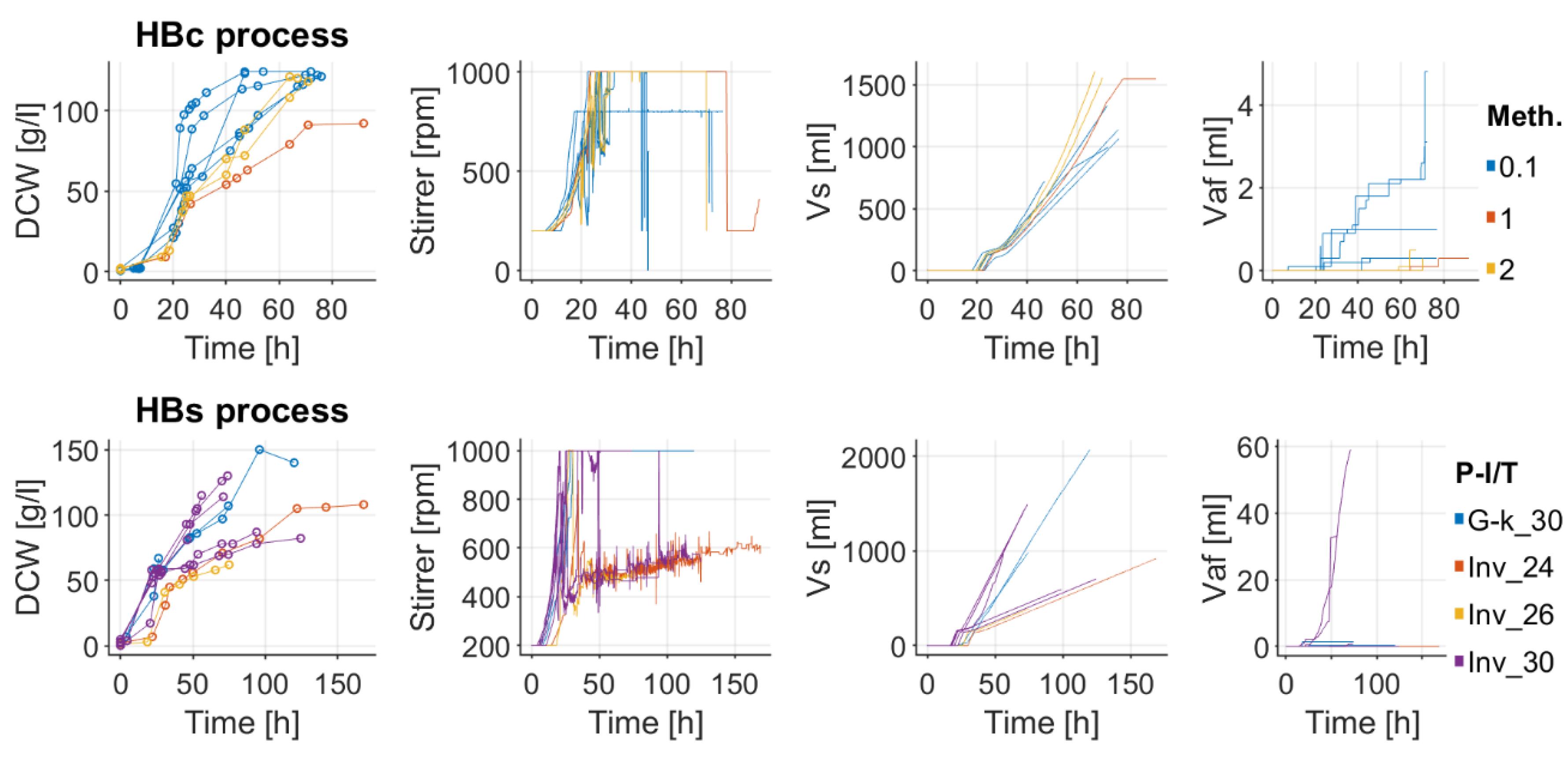
2.1. Cultivation Conditions
2.2. Off-Line Measurements
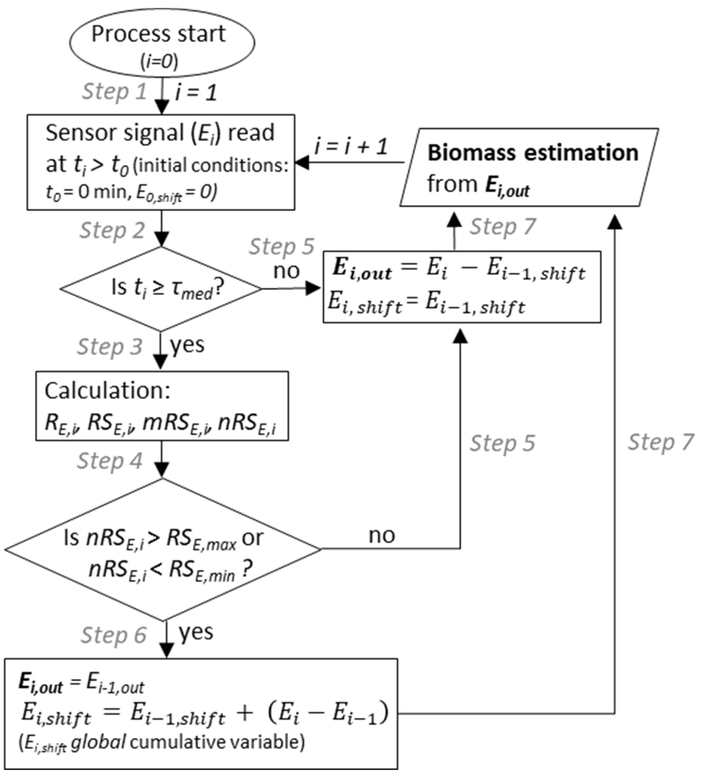
2.3. Turbidity and Permitivitty Signal Acquisition and Filtering
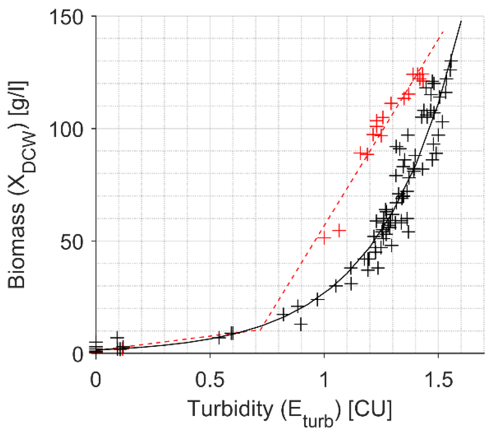
2.4. Turbidity Signal Approximation to DCW
2.5. Permittivity Signal Approximation to DCW
2.6. OUR and CPR Calculation
2.7. Estimation of Biomass Concentration from OUR, CPR and BCR
2.8. Estimation Quality Analysis
3. Results
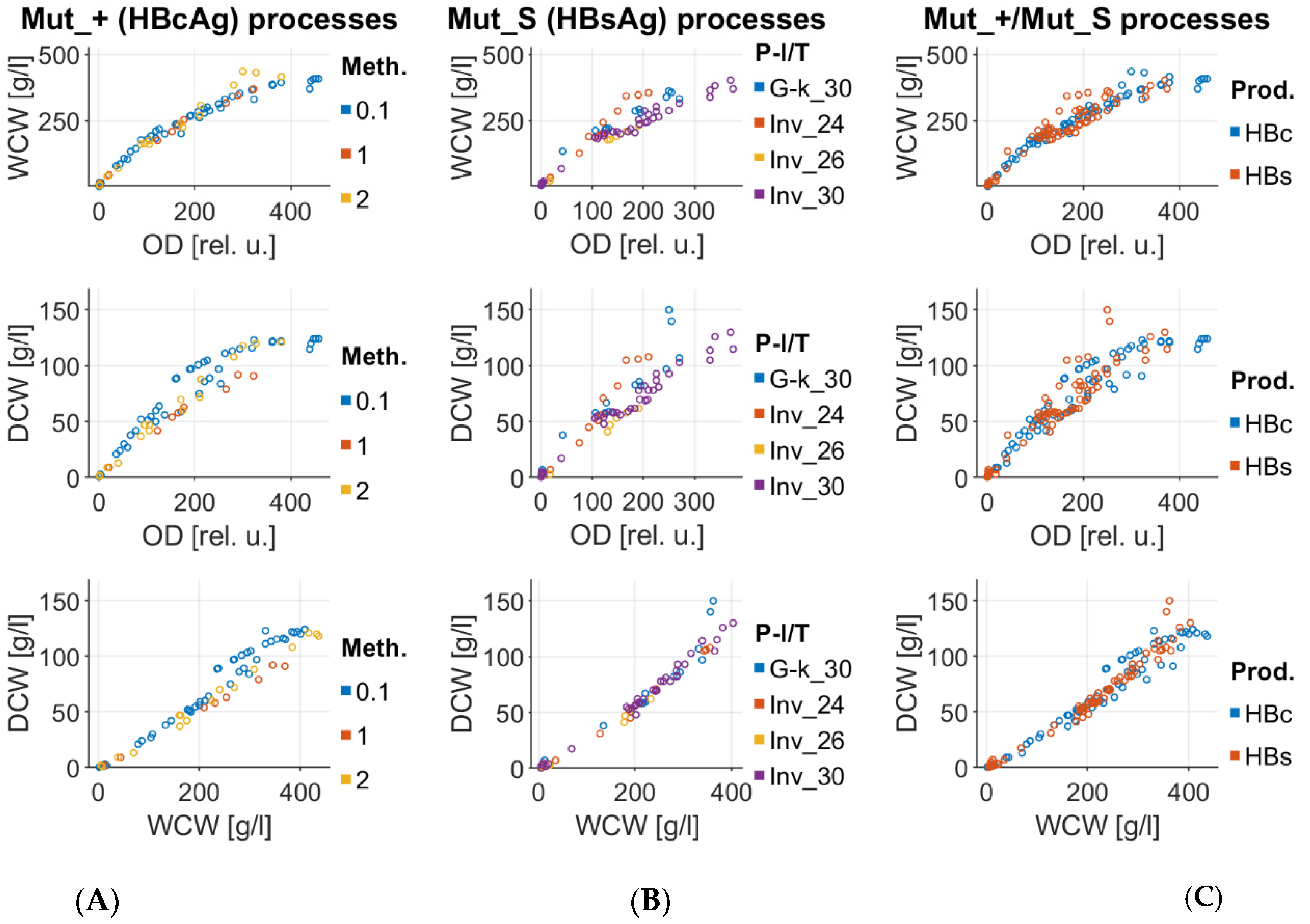
3.1. Biomass Concentration Determined Off-Line
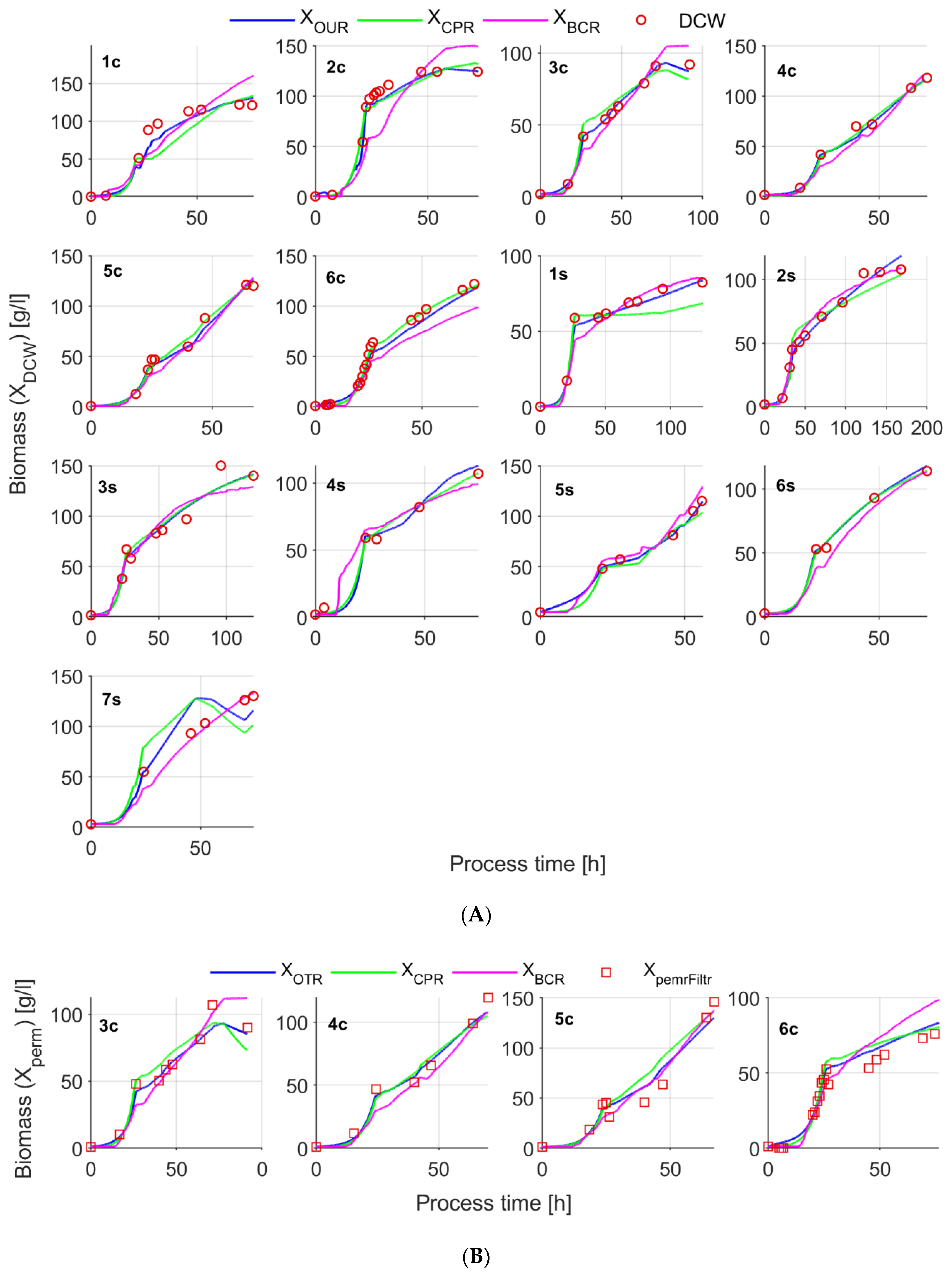
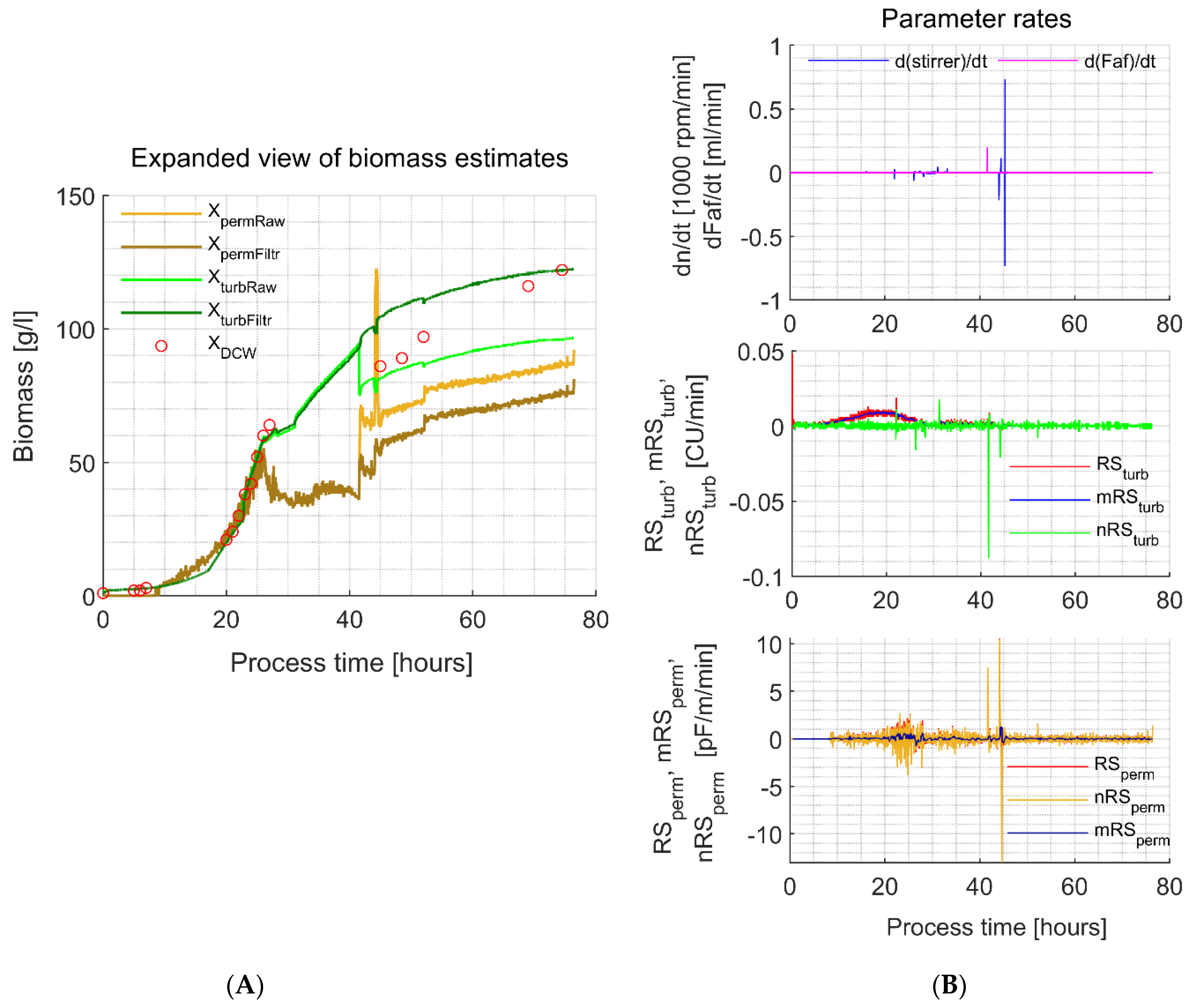
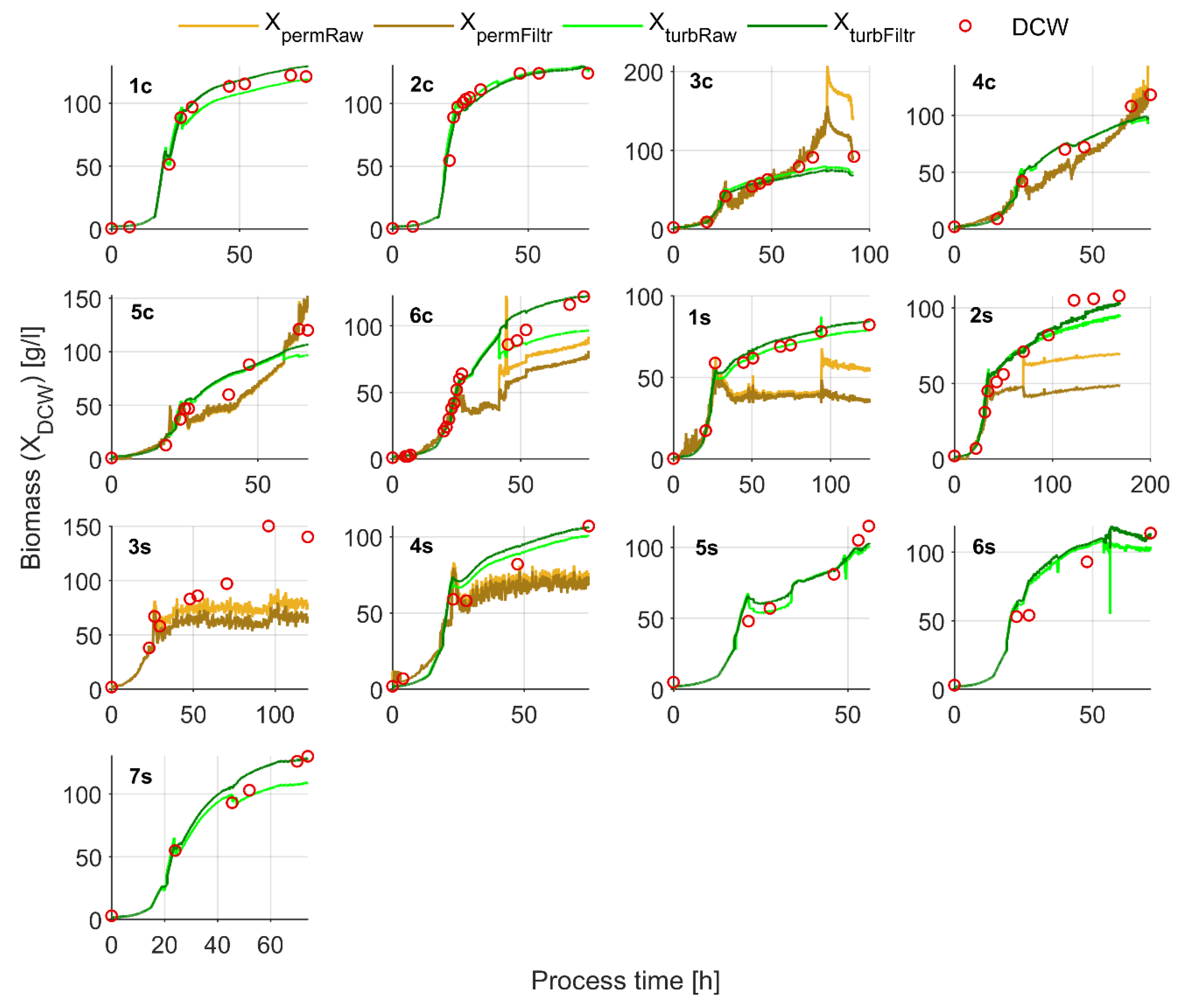
3.2. Biomass Estimates from In-Situ Turbidity and Permittivity Sensors
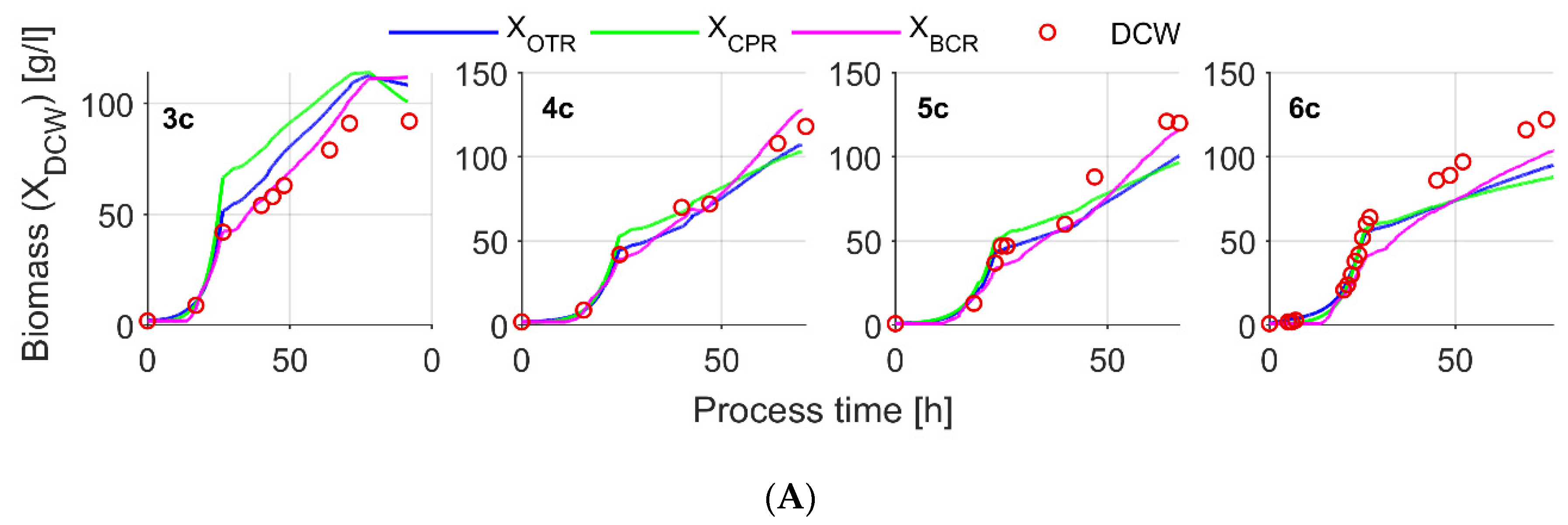
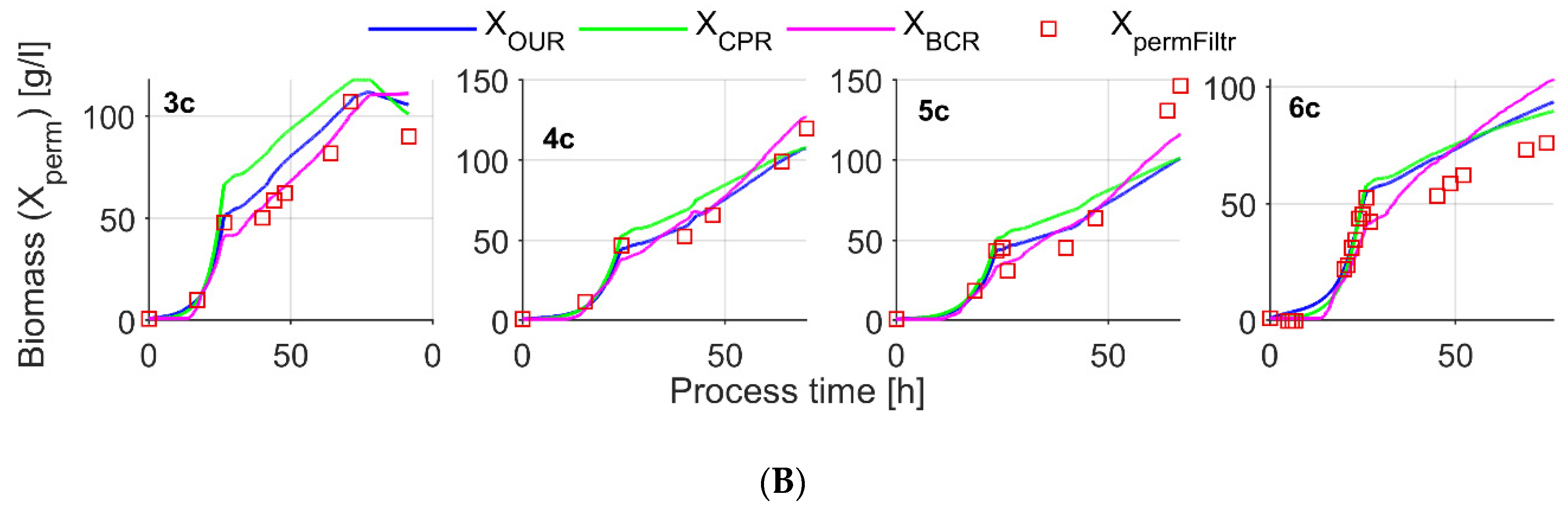
3.3. Biomass Estimation from OUR, CER and BCR Data
4. Discussion
4.1. Off-Line Biomass Detection Methods
4.2. DCW Estimation with the In-Situ Turbidity Sensor
4.3. In-Situ Permittivity (XpermFiltr) Based Biomass Estimates
4.4. Soft-Sensor-Based Biomass Estimates
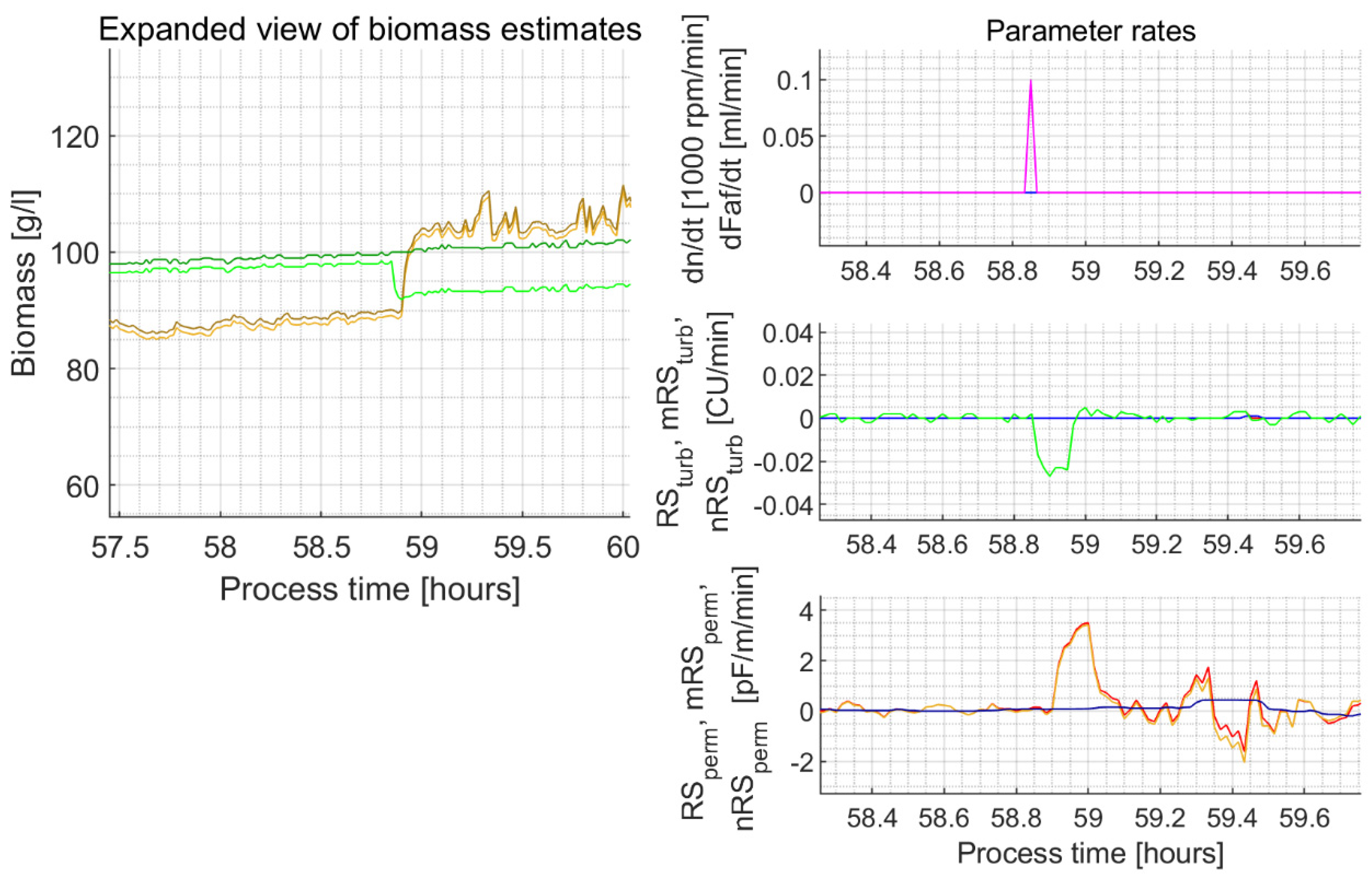
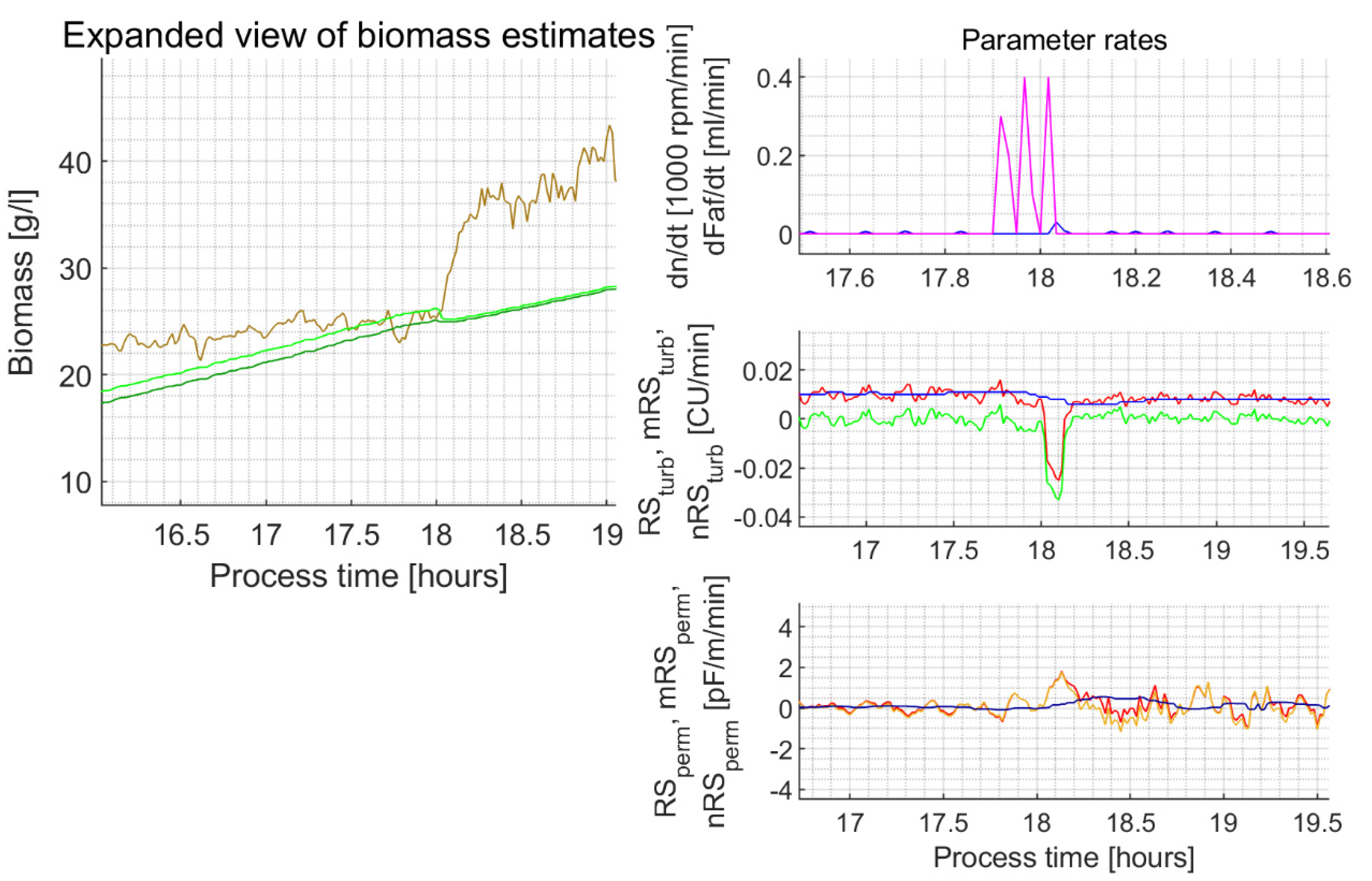
4.5. In-Situ Turbidity and Permittivity Signal Filter
4.6. Concluding Remarks
Author Contributions
Funding
Institutional Review Board Statement
Informed Consent Statement
Data Availability Statement
Acknowledgments
Conflicts of Interest
List of Symbols
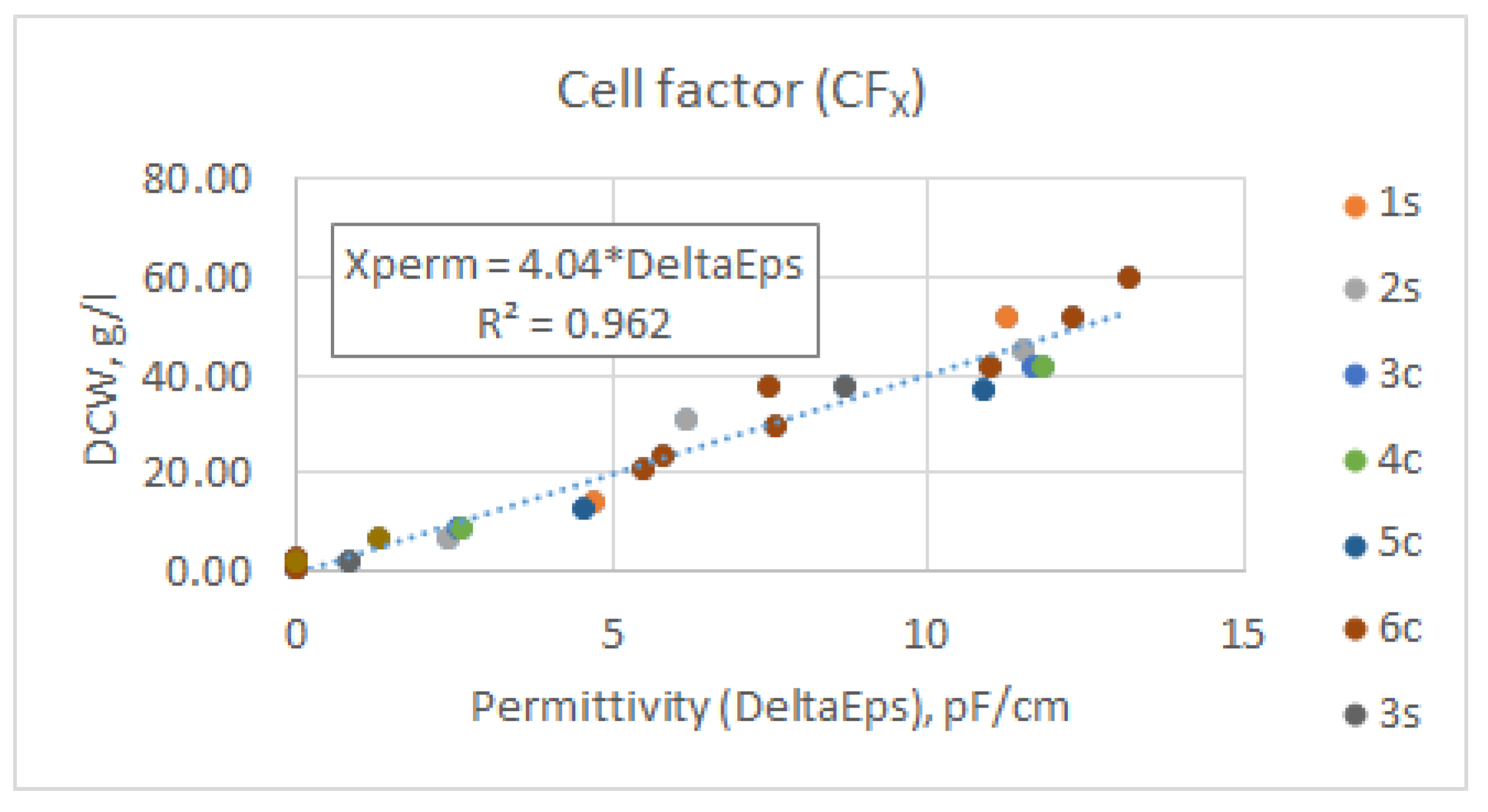
| CF | Cell factor [g/L/pF/cm] |
| HBcAg | Hepatitis B core-antigen |
| HBsAg | Hepatitis B surface-antigen |
| DO | Dissolved oxygen |
| OD | Optical density [rel. u. (relative units)] |
| DCW | Dry cell weight concentration [g/L] |
| WCW | Wet cell weight concentration [g/L] |
| GMP | Good Manufacturing Practice |
| PID | Proportional, Integral and Derivative control parameters |
| PLC | Process Logical Controller |
| SCADA | Supervisory Control and Data Acquisition |
| c | Concentration |
| O2 | Oxygen |
| CO2 | Carbon dioxide |
| N2 | Nitrogen |
| μ | Biomass growth rate [1/h] |
| Fs | Feeding rate of substrate solution [kg/h] |
| FCO2 | Carbon loss via off-gass [kg/h] |
| Fb | Alkali addition rate [kg/h] |
| Fe | Evaporation rate [kg/h] |
| Fsmp | Sampling rate [kg/h]) |
| E | Raw sensor signal (output) [units depend on the sensor] |
| Eperm | Permittivity sensor signal (output) (DeltaEps) [pF/cm] |
| Eturb | Turbidity sensor signal (output) [CU (concentration units)] |
| R | Rate |
| RS | Rate sum |
| RX | Biomass formation rate [kg(X)/kg(Culture)/h] |
| Qair | Air flow rate [slpm (standard liters per minute)] |
| QO2,enr | Oxygen flow rate [slpm (standard liters per minute)] |
| t | Process time [h] |
| τ | Period [s, min, h] |
| W | Culture mass [kg] |
| x | Total biomass weight [g, kg] |
| X | Biomass concentration [g/L, kg/L] |
| Y | Yield parameter [kg/kg] |
| Indices | |
| ATP | Adenosine triphosphate |
| i | Item number i |
| t | Time point t |
| O, O2 | Oxygen |
| C, CO2 | Carbon dioxide |
| E | Raw sensor signal (output) |
| B | Base or alkali |
| X | Biomass |
| DCW | Dry cell weight concentration |
| WCW | Wet cell weight concentration |
| af | Antifoam |
| m | Maintenance |
| S | Substrate |
| enr | Enrichment |
| Filtr | Filtrated signal |
| % | Percent |
| calibr | Calibration |
| pH | Acidity measure |
| feed | Feed solution |
| turb | Turbidity |
| perm | Permittivity |
| glyc | Glycerol |
| meth | Methanol |
| end | End measurement |
| 0 | Initial measurement |
Appendix A
Appendix B

| Column. no. (→) | 1 | 2 | 3 | 4 | 5 | 6 | 7 | 8 | 9 |
|---|---|---|---|---|---|---|---|---|---|
| Exps. | Time (h) | Max. dn/dt (rpm) | Max. d(a-foam)/dt mL/min | Max. RSn for Eturb (min) | Biomass Estimates XturbRaw0 XturbRaw1 (Diff. in %) (g(Dry Cell Weight)/L) | Biomass Estimates XturbFiltr0 XturbFiltr1 (Diff. in %) (g(Dry Cell Weight)/L) | Max. RSn for Eperm (min) | Biomass Estimates XpermRaw0XpermRaw1 (Diff. in %) (g(Dry Cell Weight)/L) | Biomass Estimates XpermFiltr0XpermFiltr1 (Diff. in %) (g(Dry Cell Weight)/L) |
| 1c | 21.3 | −97 | 0 | −0.069 | 65.08 53.6 (17.6%) | 62.3 59.1 (5.1%) | ̶ | ̶ | ̶ |
| 23.05 | 139 | 0 | +0.069 | 51.8 63.6 (22.8%) | 58.658.6(0%) | ̶ | ̶ | ̶ | |
| 27.53 | 70 | 0.9 (27.47 h) | −0.099 | 97.2 79.7 (18%) | 91.3 91.3 (0%) | ̶ | ̶ | ̶ | |
| 2c | NA | NA | NA | NA | Good filtering quality | NA | NA | NA | NA |
| 3c | 22.7 | 36 | 0 | +0.014 | 25.7 26.4 (2.7%) | 25.7 25.7 (0%) | +0.67 | NA | NA |
| 78.05 | −131 | 0.2 (77.38 h) | +0.014 | 78.7 78.0 (0.9%) | 73.8 74.0 (0.3%) | +12.3 | 140.9 206.1 (46.3%) | 155.2 152.8 (1.5%) | |
| 4c | Similar to 3c experiment | ||||||||
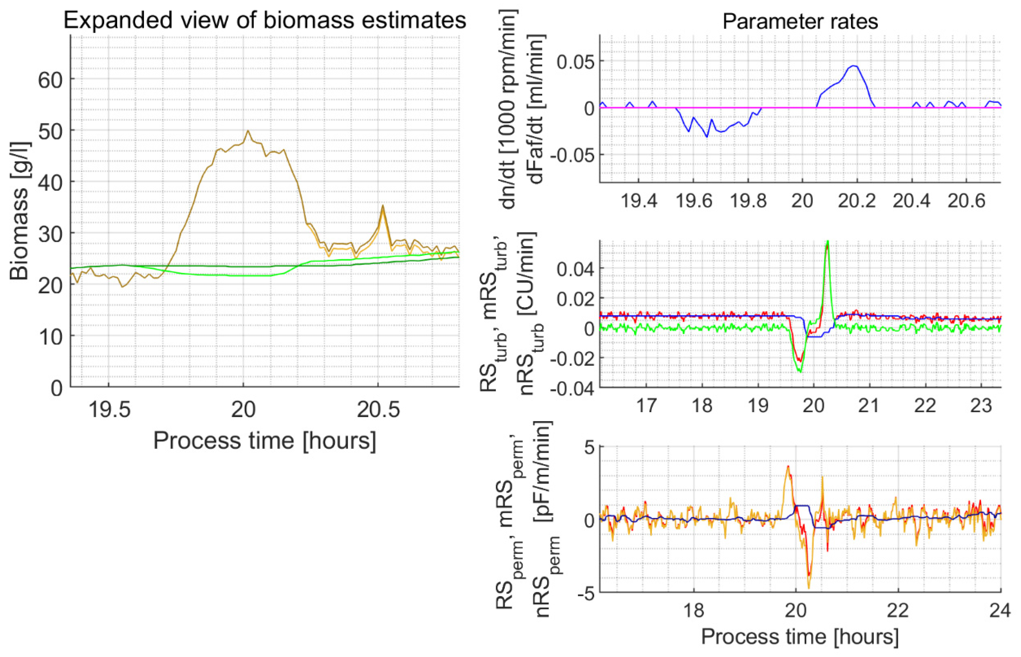
| 5c | 19.73–20.30 | NA | NA | NA | NA | NA | In the explorative experiments, the unusually lasting decrease and then the lasting increase of the stirrer rotation speed lead to a permittivity signal peak unfiltered by the proposed filter algorithm and filter parameters (Figure A3) | ||
| 58.83 | 0 | 0.1 | −0.023 | 99.5 91.8 (7.7%) | 100.0 100.0 (0%) | +3.5 | 90.1 101.1 (12.2%) | 90.1 101.1 (12.2%) | |
| 6c | 36.8 | 0 | 0.2 | −0.088 | 94.5 75.5 (20.1%) | 93.3 96.7 (3.6%) | +7.5 | 41.6 69.2 (66.3%) | 41.6 50.9 (22.4%) |
| 44.07 | −217 | 0 | −0.019 | 81.7 76.7 (6.1%) | 100.8 98.2 (2.6%) | +10.1 | 66.21 121.9 (84.1%) | 46.9 56.6 (20.7%) | |
| 44.50 | 114 | 0 | 0.0005 | 76.1 80.8 (6.2%) | 98.0 103.7 (5.8%) | −13.1 | 118.8 64.8 (45.5%) | 57.2 53.9 (5.8%) | |
| 1s | 94.03 | 62 | 0 | −0.039 | 87.4 78.0 (10.8%) | 80.6 80.6 (0%) | 3.99 | 37.7 67.9 (80.1%) | 37.7 45.2 (19.9%) |
| 4s | 18.03 | 30 | 17.9–18.02 h tree ~0.35 mL impulses of a-foam | −0.035 | 26.2 25.3 (3.4%) | 25.1 25.0 (0.4%) | 1.78 (max. reached in ~6 min) | 26.06 34.3 (31.6%) | 26.06 34.3 (31.6%) |
| 22.25 | 26 | 0 | −0.030 | 71.2 66.1 (7.2%) | 70.0 68.8 (1.7%) | +4.40 | 42.7 60.5 (41.7%) | 42.7 60.5 (41.7%) | |
| Mean difference in % | 10.3% | 1.6% | — | 51.0% | 19.5% | ||||
Appendix C

Appendix D


Appendix E
References
- Yang, Z.; Zhang, Z. Engineering strategies for enhanced production of protein and bio-products in Pichia pastoris: A review. Biotechnol. Adv. 2018, 36, 182–195. [Google Scholar] [CrossRef]
- Pichia Produced Products on the Market. Available online: https://pichia.com/science-center/commercialized-products/ (accessed on 21 November 2020).
- Dishlers, A.; Skrastina, D.; Renhofa, R.; Petrovskis, I.; Ose, V.; Lieknina, I.; Jansons, J.; Pumpens, P.; Sominskaya, I. The Hepatitis B Virus Core Variants that Expose Foreign C-Terminal Insertions on the Outer Surface of Virus-Like Particles. Mol. Biotechnol. 2015, 57, 1038–1049. [Google Scholar] [CrossRef] [PubMed]
- Kazaks, A.; Lu, I.-N.; Farinelle, S.; Ramirez, A.; Crescente, V.; Blaha, B.; Ogonah, O.; Mukhopadhyay, T.; De Obanos, M.P.; Krimer, A.; et al. Production and purification of chimeric HBc virus-like particles carrying influenza virus LAH domain as vaccine candidates. BMC Biotechnol. 2017, 17, 79. [Google Scholar] [CrossRef] [PubMed] [Green Version]
- Soares, E.; Cordeiro, R.A.; Faneca, H.; Borges, O. Polymeric nanoengineered HBsAg DNA vaccine designed in combination with β-glucan. Int. J. Biol. Macromol. 2019, 122, 930–939. [Google Scholar] [CrossRef]
- Marini, A.; Zhou, Y.; Li, Y.; Taylor, I.J.; Leneghan, D.B.; Jin, J.; Zaric, M.; Mekhaiel, D.; Long, C.A.; Miura, K.; et al. A Universal Plug-and-Display Vaccine Carrier Based on HBsAg VLP to Maximize Effective Antibody Response. Front. Immunol. 2019, 10, 2931. [Google Scholar] [CrossRef] [PubMed] [Green Version]
- Delvigne, F.; Zacchetti, B.; Fickers, P.; Fifani, B.; Roulling, F.; Lefebvre, C.; Neubauer, P.; Junne, S. Improving control in microbial cell factories: From single cell to large-scale bioproduction. FEMS Microbiol. Lett. 2018, 365, 1–11. [Google Scholar] [CrossRef]
- European Commission. EudraLex—Volume 4, Annex 2 Manufacture of Biological Active Substances and Medicinal Products for Human Use; European Commission: Brussels, Belgium, 2012; p. 4. [Google Scholar] [CrossRef]
- Takahashi, T. Applicability of Automated Cell Counter with a Chlorophyll Detector in Routine Management of Microalgae. Sci. Rep. 2018, 8, 4967. [Google Scholar] [CrossRef] [PubMed]
- Ongena, K.; Das, C.; Smith, J.L.; Gil, S.; Johnston, G. Determining Cell Number During Cell Culture using the Scepter Cell Counter. J. Vis. Exp. 2010, e2204. [Google Scholar] [CrossRef] [PubMed]
- Vees, C.A.; Veiter, L.; Sax, F.; Herwig, C.; Pflügl, S. A robust flow cytometry-based biomass monitoring tool enables rapid at-line characterization of S. cerevisiae physiology during continuous bioprocessing of spent sulfite liquor. Anal. Bioanal. Chem. 2020, 412, 2137–2149. [Google Scholar] [CrossRef] [Green Version]
- Kiviharju, K.; Salonen, K.; Moilanen, U.; Eerikäinen, T. Biomass measurement online: The performance of in situ measurements and software sensors. J. Ind. Microbiol. Biotechnol. 2008, 35, 657–665. [Google Scholar] [CrossRef]
- Biechele, P.; Busse, C.; Solle, D.; Scheper, T.; Reardon, K.F. Sensor systems for bioprocess monitoring. Eng. Life Sci. 2015, 15, 469–488. [Google Scholar] [CrossRef]
- Claßen, J.; Aupert, F.; Reardon, K.F.; Solle, D.; Scheper, P.T. Spectroscopic sensors for in-line bioprocess monitoring in research and pharmaceutical industrial application. Anal. Bioanal. Chem. 2016, 409, 651–666. [Google Scholar] [CrossRef]
- Marbà-Ardébol, A.-M.; Emmerich, J.; Muthig, M.; Neubauer, P.; Junne, S. Real-time monitoring of the budding index in Saccharomyces cerevisiae batch cultivations with in situ microscopy. Microb. Cell Factories 2018, 17, 73. [Google Scholar] [CrossRef] [Green Version]
- Zitzmann, J.; Weidner, T.; Eichner, G.; Salzig, D.; Czermak, P. Dielectric Spectroscopy and Optical Density Measurement for the Online Monitoring and Control of Recombinant Protein Production in Stably Transformed Drosophila melanogaster S2 Cells. Sensors 2018, 18, 900. [Google Scholar] [CrossRef] [PubMed] [Green Version]
- Jahic, M.; Rotticci-Mulder, J.; Martinelle, M.; Hult, K.; Enfors, S.O. Modeling of growth and energy metabolism of Pichia pastoris producing a fusion protein. Bioprocess Biosyst. Eng. 2001, 24, 385–393. [Google Scholar] [CrossRef]
- Fehrenbach, R.; Comberbach, M.; Pêtre, J. On-line biomass monitoring by capacitance measurement. J. Biotechnol. 1992, 23, 303–314. [Google Scholar] [CrossRef]
- Drieschner, T.; Ostertag, E.; Boldrini, B.; Lorenz, A.; Brecht, M.; Rebner, K. Direct optical detection of cell density and viability of mammalian cells by means of UV/VIS spectroscopy. Anal. Bioanal. Chem. 2020, 412, 3359–3371. [Google Scholar] [CrossRef]
- Noui, L.; Hill, J.; Keay, P.J.; Wang, R.Y.; Smith, T.; Yeung, K.; Habib, G.; Hoare, M. Development of a high resolution UV spectrophotometer for at-line monitoring of bioprocesses. Chem. Eng. Process. Process. Intensif. 2002, 41, 107–114. [Google Scholar] [CrossRef]
- Sandnes, J.M.; Ringstad, T.; Wenner, D.; Heyerdahl, P.; Källqvist, T.; Gislerød, H. Real-time monitoring and automatic density control of large-scale microalgal cultures using near infrared (NIR) optical density sensors. J. Biotechnol. 2006, 122, 209–215. [Google Scholar] [CrossRef] [PubMed]
- Roberts, J.; Power, A.; Chapman, J.; Chandra, S.; Cozzolino, D. The Use of UV-Vis Spectroscopy in Bioprocess and Fermentation Monitoring. Fermentation 2018, 4, 18. [Google Scholar] [CrossRef] [Green Version]
- Park, B.G.; Lee, W.G.; Chang, Y.K.; Chang, H.N. Long-term operation of continuous high cell density culture of. Bioprocess Biosyst. Eng. 1999, 21, 97. [Google Scholar] [CrossRef]
- Havlik, I.; Lindner, P.; Scheper, P.T.; Reardon, K.F. On-line monitoring of large cultivations of microalgae and cyanobacteria. Trends Biotechnol. 2013, 31, 406–414. [Google Scholar] [CrossRef] [PubMed]
- Marquard, D.; Enders, A.; Roth, G.; Rinas, U.; Scheper, T.; Lindner, P. In situ microscopy for online monitoring of cell concentration in Pichia pastoris cultivations. J. Biotechnol. 2016, 234, 90–98. [Google Scholar] [CrossRef]
- Knabben, I.; Regestein, L.; Schauf, J.; Steinbusch, S.; Büchs, J. Linear Correlation between Online Capacitance and Offline Biomass Measurement up to High Cell Densities in Escherichia coli Fermentations in a Pilot-Scale Pressurized Bioreactor. J. Microbiol. Biotechnol. 2011, 21, 204–211. [Google Scholar] [CrossRef] [Green Version]
- Sarrafzadeh, M.; Belloy, L.; Esteban, G.; Navarro, J.; Ghommidh, C. Dielectric monitoring of growth and sporulation of Bacillus thuringiensis. Biotechnol. Lett. 2005, 27, 511–517. [Google Scholar] [CrossRef] [PubMed]
- Opitz, C.; Schade, G.; Kaufmann, S.; Di Berardino, M.; Ottiger, M.; Grzesiek, S. Rapid determination of general cell status, cell viability, and optimal harvest time in eukaryotic cell cultures by impedance flow cytometry. Appl. Microbiol. Biotechnol. 2019, 103, 8619–8629. [Google Scholar] [CrossRef]
- Horta, A.C.L.; Da Silva, A.J.; Sargo, C.R.; Cavalcanti-Montaño, I.D.; Galeano-Suarez, I.D.; Velez, A.M.; Santos, M.P.; Gonçalves, V.M.; Giordano, R.C.; Zangirolami, T.C. On-Line monitoring of biomass concentration based on a capacitance sensor: Assessing the methodology for different bacteria and yeast high cell density fed-batch cultures. Braz. J. Chem. Eng. 2015, 32, 821–829. [Google Scholar] [CrossRef]
- Goldfeld, M.; Christensen, J.; Pollard, D.; Gibson, E.R.; Olesberg, J.T.; Koerperick, E.J.; Lanz, K.; Small, G.W.; Arnold, M.A.; Evans, C.E. Advanced near-infrared monitor for stable real-time measurement and control ofPichia pastorisbioprocesses. Biotechnol. Prog. 2014, 30, 749–759. [Google Scholar] [CrossRef]
- Raschmanová, H.; Zamora, I.; Borčinová, M.; Meier, P.; Weninger, A.; Mächler, D.; Glieder, A.; Melzoch, K.; Knejzlík, Z.; Kovar, K. Single-Cell Approach to Monitor the Unfolded Protein Response during Biotechnological Processes with Pichia pastoris. Front. Microbiol. 2019, 10, 335. [Google Scholar] [CrossRef]
- Konstantinov, K.; Pambayun, R.; Matanguihan, R.; Yoshida, T.; Perusicn, C.M.; Hu, W.-S. On-line monitoring of hybridoma cell growth using a laser turbidity sensor. Biotechnol. Bioeng. 1992, 40, 1337–1342. [Google Scholar] [CrossRef]
- Brignoli, Y.; Freeland, B.; Cunningham, D.; Dabros, M. Control of Specific Growth Rate in Fed-Batch Bioprocesses: Novel Controller Design for Improved Noise Management. Processes 2020, 8, 679. [Google Scholar] [CrossRef]
- Münzberg, M.; Hass, R.; Khanh, N.D.D.; Reich, O. Limitations of turbidity process probes and formazine as their calibration standard. Anal. Bioanal. Chem. 2016, 409, 719–728. [Google Scholar] [CrossRef] [Green Version]
- Katla, S.; Mohan, N.; Pavan, S.S.; Pal, U.; Sivaprakasam, S. Control of specific growth rate for the enhanced production of human interferon α2b in glycoengineered Pichia pastoris: Process analytical technology guided approach. J. Chem. Technol. Biotechnol. 2019, 94, 3111–3123. [Google Scholar] [CrossRef]
- Brunner, V.; Klöckner, L.; Kerpes, R.; Geier, D.; Becker, T. Online sensor validation in sensor networks for bioprocess monitoring using swarm intelligence. Anal. Bioanal. Chem. 2019, 412, 2165–2175. [Google Scholar] [CrossRef] [PubMed]
- Pohlscheidt, M.; Charaniya, S.; Bork, C.; Jenzsch, M.; Noetzel, T.L.; Lübbert, A. Bioprocess and Fermentation Monitoring. Encycl. Ind. Biotechnol. 2013, 2013, 1469–1492. [Google Scholar] [CrossRef]
- Galvanauskas, V.; Simutis, R.; Lübbert, A. Direct comparison of four different biomass estimation techniques against conventional dry weight measurements. Process Control Qual. 1998, 11, 119–124. [Google Scholar] [CrossRef]
- Wechselberger, P.; Sagmeister, P.; Herwig, C. Real-time estimation of biomass and specific growth rate in physiologically variable recombinant fed-batch processes. Bioprocess Biosyst. Eng. 2012, 36, 1205–1218. [Google Scholar] [CrossRef] [Green Version]
- Zhang, W.; Bevins, M.A.; Plantz, B.A.; Smith, L.A.; Meagher, M.M. Modeling Pichia pastoris growth on methanol and optimizing the production of a recombinant protein, the heavy-chain fragment C of botulinum neurotoxin, serotype A. Biotechnol. Bioeng. 2000, 70, 1–8. [Google Scholar] [CrossRef] [Green Version]
- Stelzer, I.V.; Kager, J.; Herwig, C. Comparison of Particle Filter and Extended Kalman Filter Algorithms for Monitoring of Bioprocesses. Comput. Aided Process Eng. 2017, 40, 1483–1488. [Google Scholar] [CrossRef]
- Steinwandter, V.; Zahel, T.; Sagmeister, P.; Herwig, C. Propagation of measurement accuracy to biomass soft-sensor estimation and control quality. Anal. Bioanal. Chem. 2016, 409, 693–706. [Google Scholar] [CrossRef] [Green Version]
- Tomàs-Gamisans, M.; Ferrer, P.; Albiol, J. Fine-tuning the P. pastoris iMT1026 genome-scale metabolic model for improved prediction of growth on methanol or glycerol as sole carbon sources. Microb. Biotechnol. 2017, 11, 224–237. [Google Scholar] [CrossRef] [Green Version]
- Kuprijanov, A.; Gnoth, S.; Simutis, R.; Lübbert, A. Advanced control of dissolved oxygen concentration in fed batch cultures during recombinant protein production. Appl. Microbiol. Biotechnol. 2009, 82, 221–229. [Google Scholar] [CrossRef]
- Oliveira, R.; Clemente, J.; Cunha, A.E.; Carrondo, M.J.T. Adaptive dissolved oxygen control through the glycerol feeding in a recombinant Pichia pastoris cultivation in conditions of oxygen transfer limitation. J. Biotechnol. 2005, 116, 35–50. [Google Scholar] [CrossRef]
- Jobé, A.M.; Herwig, C.; Surzyn, M.; Walker, B.; Marison, I.; Von Stockar, U. Generally applicable fed-batch culture concept based on the detection of metabolic state by on-line balancing. Biotechnol. Bioeng. 2003, 82, 627–639. [Google Scholar] [CrossRef] [PubMed]
- Van Der Heijden, R.T.J.M.; Romein, B.; Heijnen, J.J.; Hellinga, C.; Luyben, K.C.A.M. Linear constraint relations in biochemical reaction systems: II. Diagnosis and estimation of gross errors. Biotechnol. Bioeng. 1994, 43, 11–20. [Google Scholar] [CrossRef] [PubMed]
- Liu, W.-C.; Gong, T.; Wang, Q.-H.; Liang, X.; Chen, J.-J.; Zhu, P. Scaling-up Fermentation of Pichia pastoris to demonstration-scale using new methanol-feeding strategy and increased air pressure instead of pure oxygen supplement. Sci. Rep. 2016, 6, 18439. [Google Scholar] [CrossRef] [PubMed] [Green Version]
- Vanz, A.L.; Lunsdorf, H.; Adnan, A.; Nimtz, M.; Gurramkonda, C.; Khanna, N.; Rinas, U. Physiological response of Pichia pastoris GS115 to methanol-induced high level production of the Hepatitis B surface antigen: Catabolic adaptation, stress responses, and autophagic processes. Microb. Cell Factories 2012, 11, 103. [Google Scholar] [CrossRef] [Green Version]
- Gurramkonda, C.; Adnan, A.; Gäbel, T.; Lunsdorf, H.; Ross, A.; Nemani, S.K.; Swaminathan, S.; Khanna, N.; Rinas, U. Simple high-cell density fed-batch technique for high-level recombinant protein production with Pichia pastoris: Application to intracellular production of Hepatitis B surface antigen. Microb. Cell Factories 2009, 8, 13. [Google Scholar] [CrossRef] [Green Version]
- Potvin, G.; Ahmad, A.; Zhang, Z. Bioprocess engineering aspects of heterologous protein production in Pichia pastoris: A review. Biochem. Eng. J. 2012, 64, 91–105. [Google Scholar] [CrossRef]
- Grigs, O. Model Predictive Feeding Rate Control in Conventional and Single-use Lab-scale Bioreactors: A Study on Practical Application. Chem. Biochem. Eng. Q. 2016, 30, 47–60. [Google Scholar] [CrossRef]
- Mayyan, M. On-Line Estimation of Oxygen Transfer Rate with Oxygen Enriched Air using Off-Gas Sensor for Escherichia coli. Ph.D. Thesis, Clemson University, Clemson, SC, USA, 2017. [Google Scholar]
- Jenzsch, M.; Simutis, R.; Eisbrenner, G.; Stückrath, I.; Lübbert, A. Estimation of biomass concentrations in fermentation processes for recombinant protein production. Bioprocess Biosyst. Eng. 2006, 29, 19–27. [Google Scholar] [CrossRef] [PubMed]
- Niu, H.; Daukandt, M.; Rodriguez, C.; Fickers, P.; Bogaerts, P. Dynamic modeling of methylotrophic Pichia pastoris culture with exhaust gas analysis: From cellular metabolism to process simulation. Chem. Eng. Sci. 2013, 87, 381–392. [Google Scholar] [CrossRef]
- Barrigón, J.M.; Valero, F.; Montesinos-Seguí, J.L. A macrokinetic model-based comparative meta-analysis of recombinant protein production byPichia pastorisunderAOX1promoter. Biotechnol. Bioeng. 2015, 112, 1132–1145. [Google Scholar] [CrossRef]
- Flores-Cosío, G.; Herrera-López, E.J.; Arellano-Plaza, M.; Mathis, A.G.; Kirchmayr, M.; Amaya-Delgado, L. Application of dielectric spectroscopy to unravel the physiological state of microorganisms: Current state, prospects and limits. Appl. Microbiol. Biotechnol. 2020, 104, 6101–6113. [Google Scholar] [CrossRef] [PubMed]
- Steinwandter, V.; Borchert, D.; Herwig, C. Data science tools and applications on the way to Pharma 4.0. Drug Discov. Today 2019, 24, 1795–1805. [Google Scholar] [CrossRef]

| Exps.1 | Cultivation Protocol | Parameter Settings | Variable Control Range in the Process | |||
|---|---|---|---|---|---|---|
| Temperature (°C) | Aeration (Qair) (slpm) | O2 Enrich-ment | Residual Methanol 2 (g/L) | Dissolved Oxygen (DO) 3 (%) | ||
| 1c | Inv., Mut+ | 30 | 1.7 | yes | 0.05–0.1 | 35–40 |
| 2c | Inv., Mut+ | 30 | 1.7 | yes | 0.01–0.05 | 25–40 |
| 3c | Inv., Mut+ | 30 | 3.0 | yes | 0.5–1.5 | 25–30 |
| 4c | Inv., Mut+ | 30 | 3.0 | yes | 1.5–2 | 25–30 |
| 5c | Inv., Mut+ | 30 | 3.0 | yes | 1.5–2 | 25–30 |
| 6c | Inv., Mut+ | 30 | 3.0 | yes | 0.02 | 25–30 |
| 1s | Inv., MutS | 30 | 3.0 | yes | 0.01 | 20–40 |
| 2s | Inv., MutS | 24 | 3.0 | yes | 0.01 | 20–40 |
| 3s | Gurramkonda | 30 | 3.0 | no | 5–7 | 3–5 |
| 4s | Gurramkonda | 30 | 3.0 | no | 1–3 | 15–25 |
| 5s | Inv., MutS | 30 | 3.0 | yes | 0.5–2.0 | 25–30 |
| 6s | Inv., MutS | 30 | 3.0 | no | 4– 5 | 1–2 |
| 7s | Inv., MutS | 30 | 3.0 | no | 1.5–2.5 | 1–2; 20–35 |
| Datasets of Experiments | Aeration (slpm) | Fit Interval | Model Name | Model Parameters |
|---|---|---|---|---|
| Dataset 1: 3c, 4c, 5c, 6c, 1s, 2s, 4s, 5s, 6s, 7s | 3.0 | Whole region | Exponential 1 (Equation (7)) | a = 1.547, b = 2.85 |
| Dataset 2: 1c, 2c | 1.7 | Eturb ≤ 1.40 | Exponential 2 (Equation (8)) | a = 3939, b = 4.8, c = −3938, d = 4.8 |
| Eturb ≤ 0.72 | Linear (Equation (9)) | a = 10.76, b = 2.176 | ||
| Eturb > 0.72 | Linear (Equation (9)) | a = 542.3, b = −109 |
| Symbol | Unit | Value | |||
|---|---|---|---|---|---|
| Glycerol (Identified 1) | Glycerol (Reference) | Methanol (Identified 1) | Methanol (Reference) | ||
| YrOX | g/g | 0.66 | — | 4.60 | — |
| YmOX | g/g/h | 0.035 | 0.026 3 | 0.014 | 0.003 3 0.020 [17] 0.024–0.045 4 |
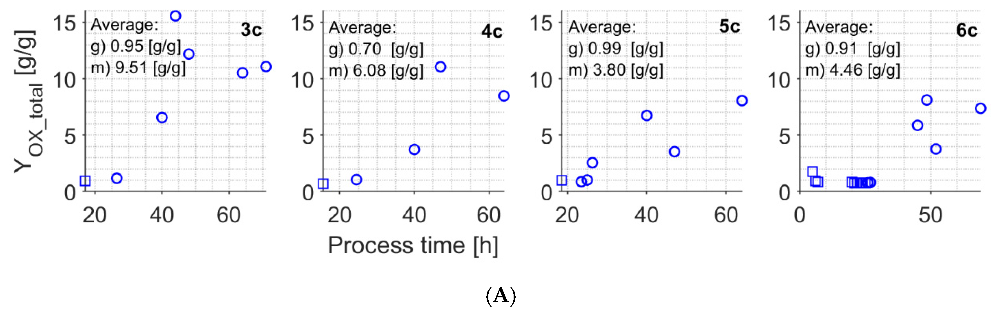
| YOX_total2 | g/g | 0.70–0.99 | 1.42–1.79 [43] | 3.80–6.08 | 5.69–6.51 [43] ~5.5 [39] |
| YrCX | g/g | 0.51 | — | 2.99 | — |
| YmCX | g/g/h | 0.068 | 0.071 [55] 0.166 3 | 0.033 | 0.282 [55] 0.029 3 |
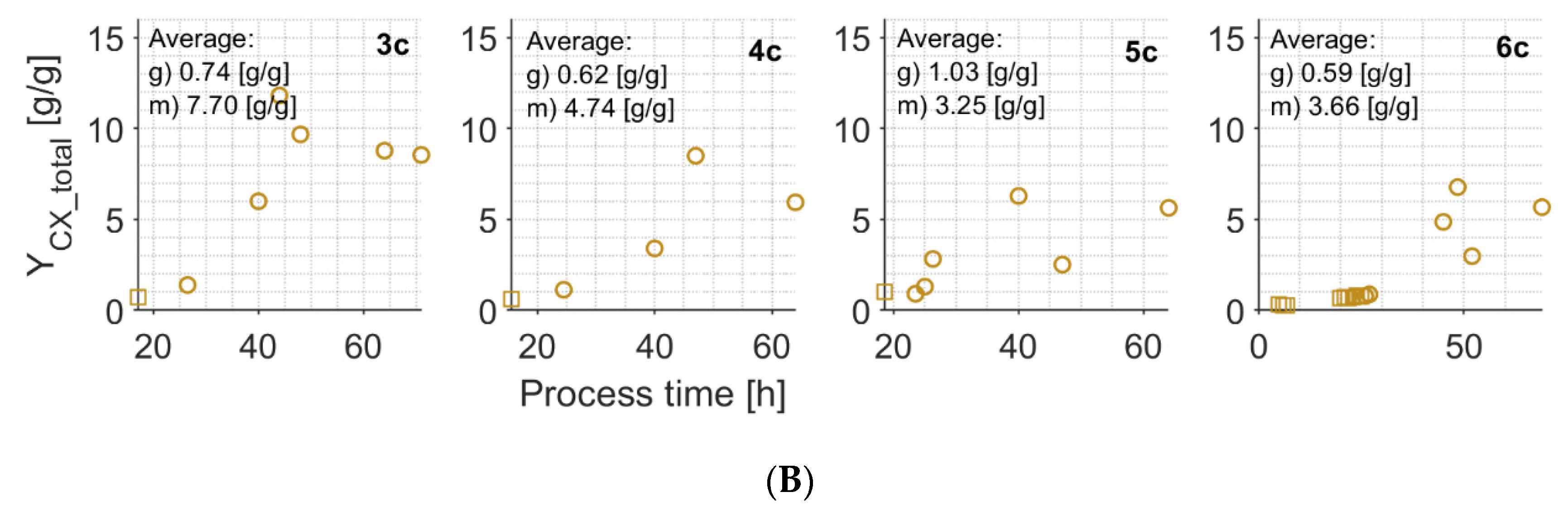
| YCX_total2 | g/g | 0.59–1.03 | 1.17–1.59 [43] | 3.25–4.74 | 4.01–4.78 [43] ~3.5 [39] |
| YrBX1 | g/g/h | 0.024 | — | 0.024 | — |
| YrBX2 | g/g/h | 0.030 | — | 0.030 | — |
| nRSE,max/nRSE,min | τsum | τmed | |
|---|---|---|---|
| For the turbidity signal | 0.01/−0.01 CU/min | 5 min | 30 min |
| For the permittivity signal | 2.5/−2.5 pF/m/min | 5 min | 30 min |
| XturbFiltr | XpermFiltr | XOUR | XCPR | XBCR | |
|---|---|---|---|---|---|
| Average NRMSE (%) | |||||
| Fit to DCW for Dataset 1 and Dataset 2 | 7 | — | — | — | — |
| Fit to DCW for Dataset 3 | 8 | 11 | 10 | 13 | 8 |
| Fit to XpermFiltr for Dataset 3 | — | — | 11 | 14 | 10 |
Publisher’s Note: MDPI stays neutral with regard to jurisdictional claims in published maps and institutional affiliations. |
© 2021 by the authors. Licensee MDPI, Basel, Switzerland. This article is an open access article distributed under the terms and conditions of the Creative Commons Attribution (CC BY) license (http://creativecommons.org/licenses/by/4.0/).
Share and Cite
Grigs, O.; Bolmanis, E.; Galvanauskas, V. Application of In-Situ and Soft-Sensors for Estimation of Recombinant P. pastoris GS115 Biomass Concentration: A Case Analysis of HBcAg (Mut+) and HBsAg (MutS) Production Processes under Varying Conditions. Sensors 2021, 21, 1268. https://doi.org/10.3390/s21041268
Grigs O, Bolmanis E, Galvanauskas V. Application of In-Situ and Soft-Sensors for Estimation of Recombinant P. pastoris GS115 Biomass Concentration: A Case Analysis of HBcAg (Mut+) and HBsAg (MutS) Production Processes under Varying Conditions. Sensors. 2021; 21(4):1268. https://doi.org/10.3390/s21041268
Chicago/Turabian StyleGrigs, Oskars, Emils Bolmanis, and Vytautas Galvanauskas. 2021. "Application of In-Situ and Soft-Sensors for Estimation of Recombinant P. pastoris GS115 Biomass Concentration: A Case Analysis of HBcAg (Mut+) and HBsAg (MutS) Production Processes under Varying Conditions" Sensors 21, no. 4: 1268. https://doi.org/10.3390/s21041268