Abstract
Compared with the standard depolarization index, indices of polarimetric purity (IPPs) have better performances to describe depolarization characteristics of targets with different roughnesses of interfaces under different incident angles, which allow us a further analysis of the depolarizing properties of samples. Here, we use IPPs obtained from different reflective interfaces as a criterion of depolarization property to characterize and classify targets covered by organic paint layers with different roughness. We select point-light source as radiation source with wavelength as 632.8 nm, and four samples, including Cu, Au, Al and Al2O3, covered by an organic paint layer with refractive index of n = 1.46 and Gaussian roughness of α = 0.05~0.25. Under different incident angles, the values of P1, P2, P3 at divided 90 × 360 grid points and their mean values in upper hemisphere have been obtained and discussed in the IPPs space. The results show that the depolarization performances of the different reflective interfaces (materials, incident angles and surface roughness) are unique in IPPs space, providing us with a new avenue to analyze and characterize different targets.
1. Introduction
Reflecting properties of different surfaces can be applied in many areas, such as 3D graphics simulation [1], biological sensing [2,3] and prediction of vegetation [4,5], which has been investigated extensively in recent years. Polarization as a powerful tool plays a great role in Mie ellipsometry [6,7] or full radiative transfer simulations [8]. In addition, polarization information of reflected light, such as degree of polarization (DoP), angle of polarization (AoP), Stokes vector et al., can provide more additional information about the targets in new aspects. When light interacts with targets, the polarization of the incident light may undergo a modification, carrying structural information of the targets. Therefore, it is important to characterize the process of the reflective polarization for exploring the polarization distributions and revealing the features of the surface, which can be used in polarization remote sensing [9,10], target detection and recognition [11,12,13,14], especially in the hidden-target identification. When the sample is not an ideal smooth surface, the reflected light will have different propagating directions, namely scattering. Reflection from a rough surface can be typically modeled using a bidirectional reflectance distribution function (BRDF) [15,16,17,18,19,20,21,22,23]. As a famous geometrical optics model, the Torrance–Sparrow (T-S) model [15] has been widely investigated and expanded to the polarized BRDF (pBRDF) models [16,17,18,19,20,21]. The Monte Carlo (MC) method has also been introduced to solve the composition of samples in fusion devices or reactive plasmas and a series of cases about polarization information [24,25,26,27,28,29,30,31,32,33], especially in photons tracking [24,25,29,30]. Wang et al. have combined the MC model with BRDF, giving birth to a flexible method to acquire the reflective polarization information from a rough surface [34]. However, these models cannot represent depolarization of the samples, which is important in real applications [35,36,37,38,39,40,41,42].
As mentioned above, depolarization is related to the structural and chemical characteristics of the samples at different physical scales, and it can be used for classifying [35,36] and analyzing samples [38,39,40,41,42]. The Mueller matrix (MM), which is composed of 4 × 4 elements namely mij, can be used to characterize the depolarization properties of mediums, and from the obtained depolarization we can obtain a set of parameters, namely IPPs (indices of polarimetric purity). The IPPs are composed of three mutually orthogonal axes P1, P2, and P3, providing a detailed description of the polarimetric purity [43,44,45]. In theory, the obtained IPPs can form a purity space. Each point in the purity space can represent a specific degree of depolarization very well, which is linked to the relative weights of the spectral components of MM directly. Meanwhile, it also provides complete information on the structure of polarimetric randomness. Given an MM, the corresponding values of P1, P2, P3 can be directly calculated [43,44,45,46,47]. In simple words, IPPs are easy to implement for discussing depolarization properties.
In this paper, we investigated the depolarization of the reflective interfaces that are composed of Cu, Au, Al and Al2O3 covered by an organic paint layer, which is a kind of common paint with a refractive index of n = 1.46 under the wavelength as 632.8 nm, and different roughness as functions of incident angles by using MC simulations. The overall depolarizations of different samples are calculated, and the results illustrate that the overall depolarization increases with increasing the roughness of organic paint layers. In addition, the metals and oxides samples show opposite dependence on incident angles, in which large incident angles may result in weak depolarization of metals, and on the contrary, result in strong depolarization of oxides. Moreover, these dependences are also varying for different metals. The exiting light from reflective interface has different IPPs with different zenithal and azimuthal directions. In other words, refractive light carries unique depolarization information with different directions. In order to better explain the depolarization characteristics of samples, we also calculate P1, P2, P3 at each divided grid point in the upper hemisphere space that include all directions of refractive light. Our results can reflect more dimensions information about depolarization of the target, which provides a new method for remote sensing and hidden target identification.
2. Methods
2.1. The IPPs of Material Media
To start, we focused on a set of three parameters, called IPPs, which provide an extended way to characterize, analyze and classify samples with different depolarization property. It is because IPPs can represent the relative statistical weight of the decomposed nondepolarizing components, providing a more accurate description of the depolarization properties of the sample. IPPs are defined as relative differences among the four eigenvalues (taken in decreasing order ) of the covariance matrix H, which can be obtained from MM by the following equation [43]:
In theory, four non-negative eigenvalues () can be obtained from the covariance matrix H, which can be used to represent the relative statistical weights of the nondepolarizing components, from which the IPPs can be defined by the following equations:
The depolarization index () can be calculated from IPPs as follows:
In general, nondepolarizing samples are characterized by = P1 = P2 = P3 = 1. The samples with = P1 = P2 = P3 = 0 are corresponding to ideal depolarizers, and there will be , where is the mean intensity coefficient. Note that, the values of IPPs will be restricted by the following inequalities:
2.2. Microfacet Theory
In general, the height field of rough surface satisfies the Gaussian distribution with variance α. The larger the variance, the rougher the surface. In addition, rough surface is assumed to be made of many microfacets, called microfacets theory, and the normal vector of each microfacet can be determined by and shown in Figure 1b, which can be calculated by sampling [34]. Then, the reflective light and refractive light of microfacets can be calculated by the Fresnel formula and normal vector of microfacet [48,49].
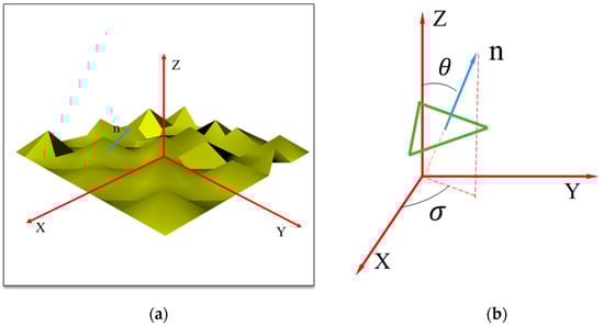
Figure 1.
(a) Surface composed of the microfacets in the XYZ coordinate system, (b) the schematics of a single microfacet.
In the tracking process of the polarized light, each beam of light propagates in global coordinate system shown in Figure 1a, and Fresnel’s law is used in the local coordinate system defined by normal vector of microfacets shown in Figure 1b. Thus, it is necessary to translate two kinds of coordinate system. The coordinate transformation can be accessed by rotating an angle [48]. The rotation matrix is , and the corresponding Mueller matrix can be expressed as follows [48].
2.3. Monte Carlo Simulation
As shown in Figure 2a, a sample is covered by some coating layers. The point-light source is emitted in the upper hemisphere. When a beam of light reaches to the coating layer with an angle of , refraction and reflection will happen. The reflected light will be collected in the upper hemisphere immediately. In contrast, the refracted light will go through a series of reflections and refractions, and can be collected in the upper hemisphere eventually, in which the upper hemisphere is divided into 90 × 360 grids with the step of 1° (in both zenithal and azimuthal directions) to collect the reflective and refractive photons. The top view of the upper hemisphere is shown in Figure 2b, in which the upper hemisphere can be divided into 90 rings according to the zenith angle (0°~90°), and combining azimuth angle (0°~360°), the detection grid can be fixed. The exiting light from the coating layers can be collected according to their concrete positions defined by the azimuth and zenith in the corresponding grid, from which their Stokes vectors in each grid can be obtained by counting and summing the received photons’ Stokes vectors.
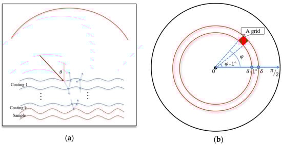
Figure 2.
(a). Model of sample covered by coating layers, (b) the top view of the upper hemisphere.
The MC method is adopted to perform the simulation [34]. In order to explore the depolarization of samples covered by organic layers, we needed to get the MM of each grid under conditions of different incident angles and roughnesses of organic layers. Thus, we have defined the direction of the incident light as 30°, 40°, 50°, 60° and 70°, four kinds of incident lights with different polarization states as = [1000], = [1100], = [1010], = [1001], respectively, the samples under organic layers as Cu, Al, Au, and Al2O3, and the roughnesses of the organic layers as 0.05~0.25 with the step of 0.05. Based on experience, we have fixed the roughness of sample as 0.2. In the simulation model, light reaching the coating layer can be traced as the following steps:
- Calculating the next layer (usually +1 or −1) to be scattered based on the number of current layer and the direction of propagation.
- Sampling the normal vector of the layer according and [34].
- Transforming polarized light from the global coordinate to the local coordinate by .
- Calculating the direction of reflected and refracted light according to the Fresnel formula and normal vector on the selected microfacet.
- Obtaining reflected and refracted light from Fresnel’s formula and MM, respectively, by , , where and are the reflective Muller matrix and the transmitting Muller matrix, respectively [34].
- Translating them from the local coordinate to the global coordinate, respectively, by ,.
- Checking whether the light has left the coating. If yes, collecting the light in the upper hemisphere. If no, back to step 1.
- Calculating MM and covariance matrix of each grid in the upper hemisphere.
- Getting the eigenvalue from the covariance matrix.
- Calculating P1, P2, P3 from .
The process of photons tracking by MC is shown in Figure 3.
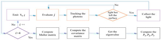
Figure 3.
The flow chart of Monte Carlo.
It should be noted that our simulation was based on two assumptions: (1) the scale of microfacet is much larger than the incident wavelength, which means the geometry optics can be applied; (2) the coating is so thin that the absorption can be ignored.
3. Results and Discussion
3.1. Comparing with BRDF Model
To demonstrate the accuracy and validity of the simulation model, we compared the results of reflection from a copper surface obtained by MC simulation and experiment-based BRDF model included in the SCATMECH [50]. Here, it should be noted that the SCATMECH is a light scattering library and published by the NIST in 2017 [50], which has been verified in many experiments. In both simulation schemes, the refractive index of copper and the surface roughness parameters are set as 0.27 + 3.40i and αx = αy = 0.2, respectively, and the incident nonpolarized light (with the wavelength of 632.8nm and the incident angle of 40°) is set as Sin = [1000] with 10 million emitted photons every time. The results of our MC model and the experiment-based BRDF model are plotted in the top and bottom panels in Figure 4, respectively. It is obvious that the reflective polarization patterns of I, Q, U, V, AoP and DoP obtained by our MC model agree well with those obtained by analytical BRDF model, which can verify the accuracy and validity of our model.
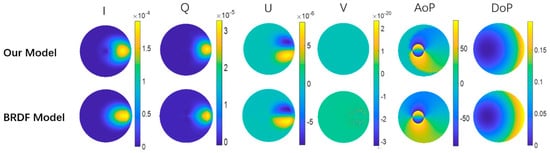
Figure 4.
Comparison of the results obtained by our model and the analytical bidirectional reflectance distribution function (BRDF) model.
3.2. Influence of Roughness
First, we chose samples (Cu, Al, Al2O3, Au) covered by organic paint layers as different reflective interfaces, in which the organic paint layer is a common paint and we assume it is a pure substance whose refractive index is 1.46 under the incident wavelength of 632.8nm. We would investigate the dependence of P1, P2, and P3 on the roughness of the organic paint layer. In the simulation, the roughness αx = αy ranges from 0.05 to 0.25 with step of 0.05. The incident angle and wavelength of light are set as 632.8 nm and 50° in the upper hemisphere, respectively. We have investigated four samples, including Cu (n = 0.27 + 3.40i), Al (n = 1.4482 + 7.53i), Au (n = 0.18 + 3.43i), and Al2O3 (n = 1.77), which are covered by an organic paint layer. The number of emitted photons is 10 million to ensure the accuracy of our MC simulation.
To study the overall depolarization property, we calculated the average values of P1, P2, and P3 at all physically feasible points [46] in the upper hemisphere of reflective interface, as shown in Figure 5. It can be observed that P1, P2, and P3 form IPPs space, in which the point (1, 1, 1) represents nondepolarizing samples and the other points represent depolarizing samples. In other words, the intrinsic depolarizing mechanisms can be demonstrated according to the coordinate in the IPPs space. Figure 5 shows that the values of P1, P2, and P3 gradually decrease with increasing roughness, indicating the depolarization of the samples increases with the increasing roughness. It is because light will be scattered rather than reflected at a rough surface, leading to depolarization of light. In addition, we can see that the calculated results of Cu in IPPs space are closer to that of Au, while far away from those of Al and Al2O3. This phenomenon could be attributed to the refractive index of the samples. As shown above, the refractive index of Cu is similar to that of Au, but quite different from those of Al and Al2O3. Therefore, we may get different distributions in the IPPs space for different samples, making it possible to classify the samples.
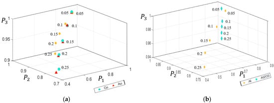
Figure 5.
The overall distributions of P1, P2, P3 corresponding to different roughnesses (a) samples as Cu, Au, Al; (b) samples as Al, Al2O3.
In order to further demonstrate the advantages of IPPs, we calculated the values of P1, P2, and P3 at each grid in the upper hemisphere when the surface roughness of organic paint layer is αx = αy = 0.05, 0.10, 0.15, 0.20, and 0.25, as shown in Figure 6. Here, we take the sample of Cu as an example. The points at which the values of P1, P2, and P3 equal zero means that eigenvalues derived from the covariance matrix H are negative, called physically unfeasible points [46]. The number of these feasible points increases but the values are decreasing with increasing roughness, which means the average value is decreasing for all physically feasible points when the roughness increases. It is consistent with Figure 5. From the simulation results, we can obtain particular depolarization information of the sample from the physically feasible points. For example, the values of P1, P2, and P3 in the point of (60, 0) decrease with increasing roughness, but are always bigger than those in the point of (60, 60). It means that the MM for the latter case has more depolarization components in characteristic decomposition, which reflects the different points in the upper hemisphere having different depolarization components. In other words, light received at different points in the upper hemisphere undergoes various coding by the sample. This characteristic makes it more difficult for us to classify the samples by using the values of P1, P2, and P3 at each grid in the upper hemisphere than by using their average values’ distributions in IPPs space.
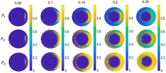
Figure 6.
P1, P2, P3 of each grid in the upper hemisphere with the changing roughness of Cu targets.
3.3. Influence of Incident Angle
It is well known that the scattering of light at an irregular structure is highly dependent on the incident angle. Therefore, the dependences of depolarization of samples on the incident angles were investigated. Here, we chose the same reflective interface, but the surface roughness of the organic paint layer was fixed as αx = αy = 0.2. The incident angles are 30°, 40°, 50°, 60° and 70°. The calculated overall distributions of P1, P2, and P3 in IPPs space are shown in Figure 7.
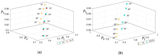
Figure 7.
The overall distributions of P1, P2, P3 corresponding to different incident angles: (a) samples as Cu, Au, Al; (b) samples as Al, Al2O3.
For metals, the results show that their depolarization properties decrease with the increasing incident angles. It is because light collected at most grids has smaller scattering components with increasing incident angles. On the contrary, oxides, such as Al2O3, hold opposite results that increasing incident angles result in more depolarization. These results illustrate that metals and oxides have different dependence of depolarization characteristics on incident angles, which makes it possible for us to classify samples.
Similarly, the values of P1, P2, and P3 at each grid in the upper hemisphere is not significantly dependent on the incident angles, as shown in Figure 8. Here, we still take the sample of Cu as an example. It can be seen that the number of physically unfeasible points slightly decreases with the increasing incident angles, and the physically feasible points have a tendency of spreading towards the center of the circle under a large incident angle. The depolarization performances at different grids are different. In addition, the P1, P2, P3 of the same grid are different, which is because the P1, P2, P3 as the relative differences of different pure systems mapped from the reflective interface depend on the inherent attribute of reflective interface, which can be used for analyzing IPPs decomposition of reflective interface and exploring the composition of reflective interface. Combining the distribution patterns of P1, P2, P3 and the IPPs space has significant advantages in classifying the depolarization characteristics of samples.
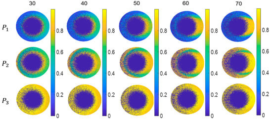
Figure 8.
P1, P2, P3 of each grid in the upper hemisphere with the incident angle change for the Cu target.
4. Conclusions
In this paper, we have emphasized the interest of using IPPs as a criterion for characterization and classification of samples covered by organic paint layers. On one hand, the IPPs carry unique depolarization information of samples, thus leading the unique distributions of overall depolarization for different samples in IPPs space. The distributions of Cu, Al, Au, Al2O3 with different incident angles and roughnesses of organic paint layers were investigated and discussed. On the other hand, the IPPs of each grid vary, which represents that the light coded by samples vary in different directions. These have exhibited the significant potential of using IPPs for target detection and remote sensing, especially the identification of the hidden target.
Author Contributions
Conceptualization, D.L., J.G. and Z.G.; methodology, Y.S., D.L. and K.G.; software, D.L.; investigation, Y.S., X.B., J.G., and K.G.; writing—original draft preparation, D.L. and X.B.; writing—review and editing, Z.G. and K.G.; supervision, Z.G.; funding acquisition, Z.G. All authors have read and agreed to the published version of the manuscript.
Funding
This research was funded by National Natural Science Foundation of China (61775050, 61971177, 11804073), Fundamental Research Funds for the Central Universities (PA2019GDZC0098).
Acknowledgments
We would like to express our great thanks for the discussions and help from Ying Zheng and Yu Lu from 713th Institute, China Shipbuilding Industry Corporation (CSIC).
Conflicts of Interest
The authors declare no conflict of interest.
References
- Cula, O.G.; Dana, K.J. 3D texture recognition using bidirectional feature histograms. Int. J. Comput. Vis. 2004, 59, 33–60. [Google Scholar] [CrossRef]
- Hu, J.C.; Zhang, C.C.; Li, X.; Du, X. An Electrochemical Sensor Based on Chalcogenide Molybdenum Disulfide-Gold-Silver Nanocomposite for Detection of Hydrogen Peroxide Released by Cancer Cells. Sensors 2020, 20, 6817. [Google Scholar] [CrossRef]
- Xia, J.J.; Yao, G. Angular distribution of diffuse reflectance in biological tissue. Appl. Opt. 2007, 46, 6552–6560. [Google Scholar] [CrossRef]
- Qi, H.; Zhu, B.; Wu, Z.; Liang, Y.; Li, J.; Wang, L.; Chen, T.; Lan, Y.; Zhang, L. Estimation of Peanut Leaf Area Index from Unmanned Aerial Vehicle Multispectral Images. Sensors 2020, 20, 6732. [Google Scholar] [CrossRef] [PubMed]
- Hegedus, R.; Barta, A.; Bernath, B.; Meyer-Rochow, V.B.; Horvath, G. Imaging polarimetry of forest canopies: How the azimuth direction of the sun, occluded by vegetation, can be assessed from the polarization pattern of the sunlit foliage. Appl. Opt. 2007, 46, 6019–6032. [Google Scholar] [CrossRef] [PubMed]
- Hayashi, Y.; Tachibana, K. Mie-Scattering Ellipsometry for Analysis of Particle Behaviors in Processing Plasmas. Jpn. J. Appl. Phys. 1994, 33, L476. [Google Scholar] [CrossRef]
- Groth, S.; Greiner, F.; Tadsen, B.; Piel, A. Kinetic Mie ellipsometry to determine the time-resolved particle growth in nanodusty plasmas. J. Phys. D Appl. Phys. 2015, 46, 465203. [Google Scholar] [CrossRef]
- Kirchschlager, F.; Wolf, S.; Greiner, F.; Groth, S.; Labdon, A. In-situ analysis of optically thick nanoparticle clouds. Appl. Phys. Lett. 2017, 110, 173106. [Google Scholar] [CrossRef]
- Agnoil, G.C.; Cacciari, M.; Garutti, C.; Lenzi, P. Ship detection performance using simulated dual-polarization radarsat constellation mission data. Int. J. Remote Sens. 2015, 36, 1705–1727. [Google Scholar]
- Wang, X.Y.; Hu, T.W.; Li, D.K.; Guo, K.; Gao, J.; Guo, Z.Y. Performances of polarization-retrieve imaging in stratified dispersion media. Remote Sens. 2020, 12, 2895. [Google Scholar] [CrossRef]
- Xu, F.; Wang, H.P.; Jin, Y.Q.; Liu, X.Q.; Wang, R.; Deng, Y. Impact of cross-polarization isolation on polarimetric target decomposition and target detection. Radio Sci. 2015, 50, 327–338. [Google Scholar] [CrossRef]
- Wang, Y.T.; Ainsworth, T. Assessment of System Polarization Quality for Polarimetric SAR Imagery and Target Decomposition. IEEE Trans. Geosci. Remote Sens. 2011, 49, 1755–1771. [Google Scholar] [CrossRef]
- Wolff, L.B. Polarization-based material classification from specular reflection. IEEE Trans. Pattern Anal. Mach. Intell. 1990, 12, 1059–1071. [Google Scholar] [CrossRef]
- Wolff, L.B.; Boult, T.E. Constraining object features using a polarization reflectance model. IEEE Trans. Pattern Anal. Mach. Intell. 1991, 13, 635–657. [Google Scholar] [CrossRef]
- Torrance, K.E.; Sparrow, E.M. Theory for off-specular reflection from roughened surfaces. J. Opt. Soc. Am. 1967, 57, 1105–1114. [Google Scholar] [CrossRef]
- Zhang, Y.; Zhang, Y.; Zhao, H.J.; Wang, Z.Y. Improved atmospheric effects elimination method for pBRDF models of painted surfaces. Opt. Express 2017, 25, 16458–16475. [Google Scholar] [CrossRef] [PubMed]
- Priest, R.G.; Meier, S.R. Polarimetric microfacet scattering theory with applications to absorptive and reflective surfaces. Opt. Eng. 2002, 41, 988–993. [Google Scholar] [CrossRef]
- Wang, K.; Zhu, J.P.; Liu, H.; Du, B.Z. Expression of the degree of polarization based on the geometrical optics pBRDF model. J. Opt. Soc. Am. A 2017, 32, 259–263. [Google Scholar] [CrossRef] [PubMed]
- Wellems, D.; Ortega, S.; Bowers, D.; Boger, J.; Fetrow, M. Long wave infrared polarimetric model: Theory, measurements and parameters. J. Opt. A Pure Appl. Opt. 2006, 8, 914–925. [Google Scholar] [CrossRef]
- Renhorn, I.G.E.; Hallberg, T.; Boreman, G.D. Efficient polarimetric BRDF model. Opt. Express 2015, 23, 31253–31273. [Google Scholar] [CrossRef]
- Hyde, M.W.; Schmidt, J.D.; Havrilla, M.J. A geometrical optics polarimetric bidirectional reflectance distribution function for dielectric and metallic surfaces. Opt. Express 2009, 17, 22138–22153. [Google Scholar] [CrossRef] [PubMed]
- Ashikhmin, M.; Shirley, P. An anisotropic phong brdf model. J. Graph. Tools 2000, 5, 25–32. [Google Scholar] [CrossRef]
- Lai, Q.Z.; Liu, B.; Zhao, J.M.; Zhao, Z.W.; Tan, J.Y. BRDF characteristics of different textured fabrics in visible and near-infrared band. Opt. Express 2020, 28, 3561–3575. [Google Scholar] [CrossRef] [PubMed]
- Fields, A.P.; Cohen, A.E. Optimal tracking of a Brownian particle. Opt. Express 2012, 20, 22585–22601. [Google Scholar] [CrossRef]
- Xu, Q.; Guo, Z.; Tao, Q.; Jiao, W.; Wang, X.; Qu, S.; Gao, J. Transmitting characteristics of the polarization information under seawater. Appl. Optics. 2015, 54, 6584–6588. [Google Scholar] [CrossRef]
- Li, M.; Lu, P.F.; Yu, Z.Y.; Yan, L.; Chen, Z.H.; Yang, C.H.; Luo, X. Vector Monte Carlo simulations on atmospheric scattering of polarization qubits. J. Opt. Soc. Am. A 2013, 30, 448–454. [Google Scholar] [CrossRef]
- Garcia, R.D.M. Fresnel boundary and interface conditions for polarized radiative transfer in a multilayer medium. J. Quant. Spectrosc. Radiat. Transf. 2012, 113, 306–317. [Google Scholar] [CrossRef]
- Xu, Q.; Guo, Z.; Tao, Q.; Jiao, W.; Qu, S.; Gao, J. Multi-spectral characteristics of polarization retrieve in various atmospheric conditions. Opt. Commun. 2015, 339, 167–170. [Google Scholar] [CrossRef]
- Tao, Q.; Sun, Y.; Shen, F.; Xu, Q.; Gao, J.; Guo, Z.Y. Active imaging with the aids of polarization retrieve in turbid media system. Opt. Commun. 2016, 359, 405–410. [Google Scholar] [CrossRef]
- Kattawar, G.W.; Plass, G.N.; Guinn, J.A., Jr. Monte Carlo calculations of the polarization of radiation in the earth’s atmosphere-ocean system. J. Phys. Oceanogr. 1973, 3, 353–372. [Google Scholar] [CrossRef]
- Hu, T.; Shen, F.; Wang, K.; Guo, K.; Liu, X.; Wang, F.; Peng, Z.; Cui, Y.; Sun, R.; Ding, Z.; et al. Broad-Band Transmission Characteristics of Polarizations in Foggy Environments. Atmosphere 2019, 10, 342. [Google Scholar] [CrossRef]
- Xu, M. Electric field Monte Carlo simulation of polarized light propagation in turbid media. Opt. Express 2004, 12, 6530–6539. [Google Scholar] [CrossRef] [PubMed]
- Zhao, J.M.; Tan, J.Y.; Liu, L.H. Monte Carlo method for polarized radiative transfer in gradient-index media. J. Quant. Spectrosc. Radiat. Transf. 2014, 152, 114–126. [Google Scholar] [CrossRef]
- Wang, C.; Gao, J.; Yao, T.T.; Wang, L.M.; Sun, Y.X.; Xie, Z.; Guo, Z.Y. Acquiring reflective polarization from arbitrary multi-layer surface based on Monte Carlo simulation. Opt. Express 2016, 9, 9397–9411. [Google Scholar] [CrossRef] [PubMed]
- Zhang, X.D.; Stramski, D.; Reynolds, R.A.; Blocker, E.R. Light scattering by pure water and seawater: The depolarization ratio and its variation with salinity. Appl Opt. 2019, 58, 991–1004. [Google Scholar] [CrossRef]
- Xu, Y.; Wang, Z.; Zhang, W.H. Depolarization effect in light scattering of single gold nanosphere. Opt. Express 2020, 28, 24275–24284. [Google Scholar] [CrossRef]
- Tudor, T. On the enpolarization/depolarization effects of deterministic devices. Opt. Lett. 2018, 43, 5234–5237. [Google Scholar] [CrossRef]
- Sato, K.; Okamoto, H.; Ishimoto, H. Modeling the depolarization of space-borne lidar signals. Opt. Express 2019, 27, A117–A132. [Google Scholar] [CrossRef]
- Bi, L.; Lin, W.H.; Liu, D.; Zhang, K.J. Assessing the depolarization capabilities of nonspherical particles in a super-ellipsoidal shape space. Opt. Express 2018, 26, 1726–1742. [Google Scholar] [CrossRef]
- Thomas, A. Evolution of transmitted depolarization in diffusely scattering media. J. Opt. Soc. Am. A 2020, 37, 980–987. [Google Scholar]
- Callum, M. Characterizing the depolarization of circularly polarized light in turbid scattering media. J. Opt. Soc. Am. A 2018, 35, 2104–2110. [Google Scholar]
- Pierangelo, A.; Nazac, A.; Benali, A.; Validire, P.; Cohen, H.; Novikova, T.; Ibrahim, B.H.; Manhas, S.; Fallet, C.; Antonelli, M.R.; et al. Polarimetric imaging of uterine cervix: A case study. Opt. Express 2013, 21, 14120–14130. [Google Scholar] [CrossRef]
- Shen, F.; Zhang, M.; Guo, K.; Zhou, H.P.; Peng, Z.Y.; Cui, Y.M.; Wang, F.; Guo, Z.Y. The depolarization performances of scattering systems based on the Indices of Polarimetric Purity. Opt. Express 2019, 27, 28337–28349. [Google Scholar] [CrossRef]
- José, I.S.; Gil, J.J. Invariant indices of polarimetric purity: Generalized indices of purity for n× n covariance matrices. Opt. Commun. 2011, 284, 38–47. [Google Scholar] [CrossRef]
- Gil, J.J. Components of purity of a three-dimensional polarization state. J. Opt. Soc. Am. A 2016, 33, 40–43. [Google Scholar] [CrossRef] [PubMed]
- Tariq, A.; He, H.H.; Li, P.C.; Ma, H. Purity-depolarization relations and the components of purity of a Mueller matrix. Opt. Express 2019, 27, 22645–22662. [Google Scholar] [CrossRef] [PubMed]
- Gil, J.J.; Ossikovski, R. Polarized Light and the Mueller Matrix Approach; CRC Press: Boca Raton, FL, USA, 2016. [Google Scholar]
- Goldstein, D. Polarized Light (Second Edition); Marcel Dekker Inc.: New York, NY, USA, 2003. [Google Scholar]
- Michael, B.; Decusatis, C.M.; Enoch, J.; MacDonald, C. Handbook of Optics; McGraw-Hill: New York, NY, USA, 2009. [Google Scholar]
- Germer, T. SCATMECH v 7.0: Polarized Light Scattering C++ Class Library; NIST: Gaithersburg, MD, USA, 2017. [Google Scholar]


Publisher’s Note: MDPI stays neutral with regard to jurisdictional claims in published maps and institutional affiliations. |
© 2021 by the authors. Licensee MDPI, Basel, Switzerland. This article is an open access article distributed under the terms and conditions of the Creative Commons Attribution (CC BY) license (http://creativecommons.org/licenses/by/4.0/).