Research on the Prediction of Green Plum Acidity Based on Improved XGBoost


Abstract
1. Introduction
2. Experiments
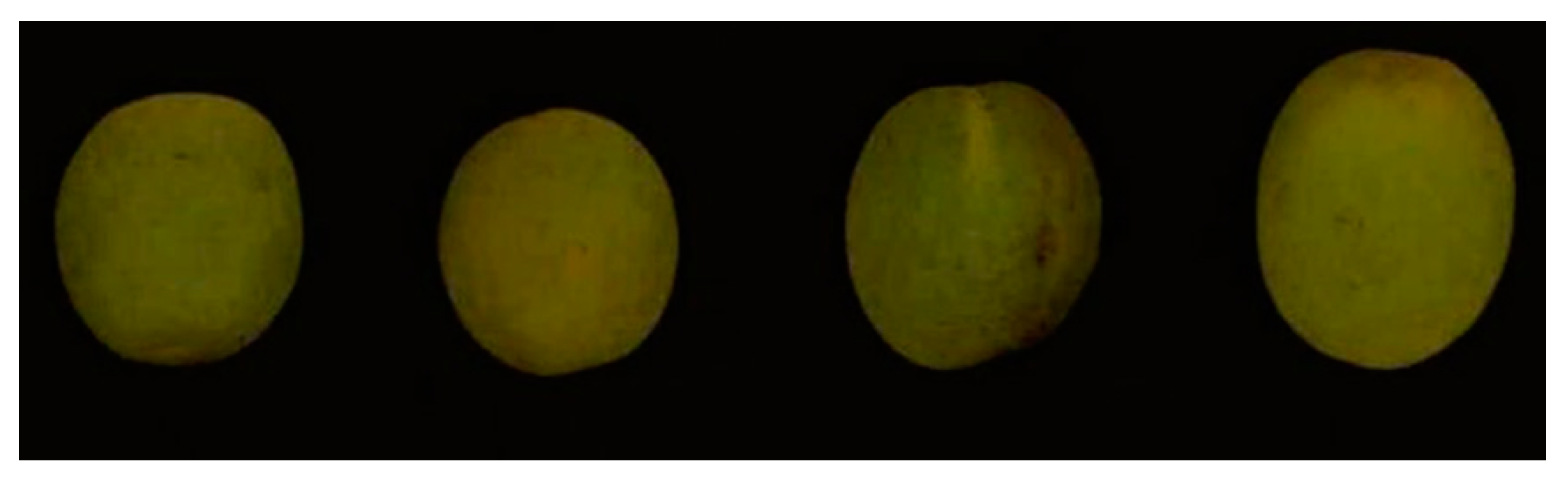
2.1. Green Plum Samples
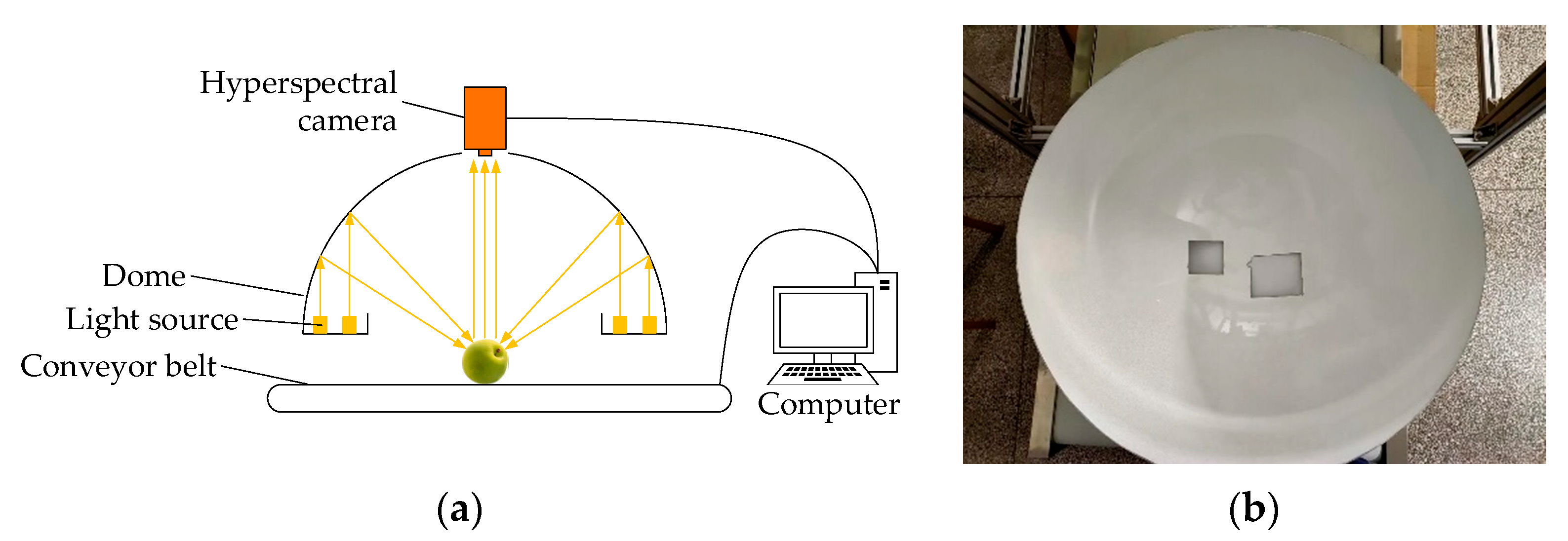
2.2. Equipment
2.3. Hyperspectral Data Acquisition
2.4. Green Plum pH Testing
2.5. Image Processing
3. Model Establishment
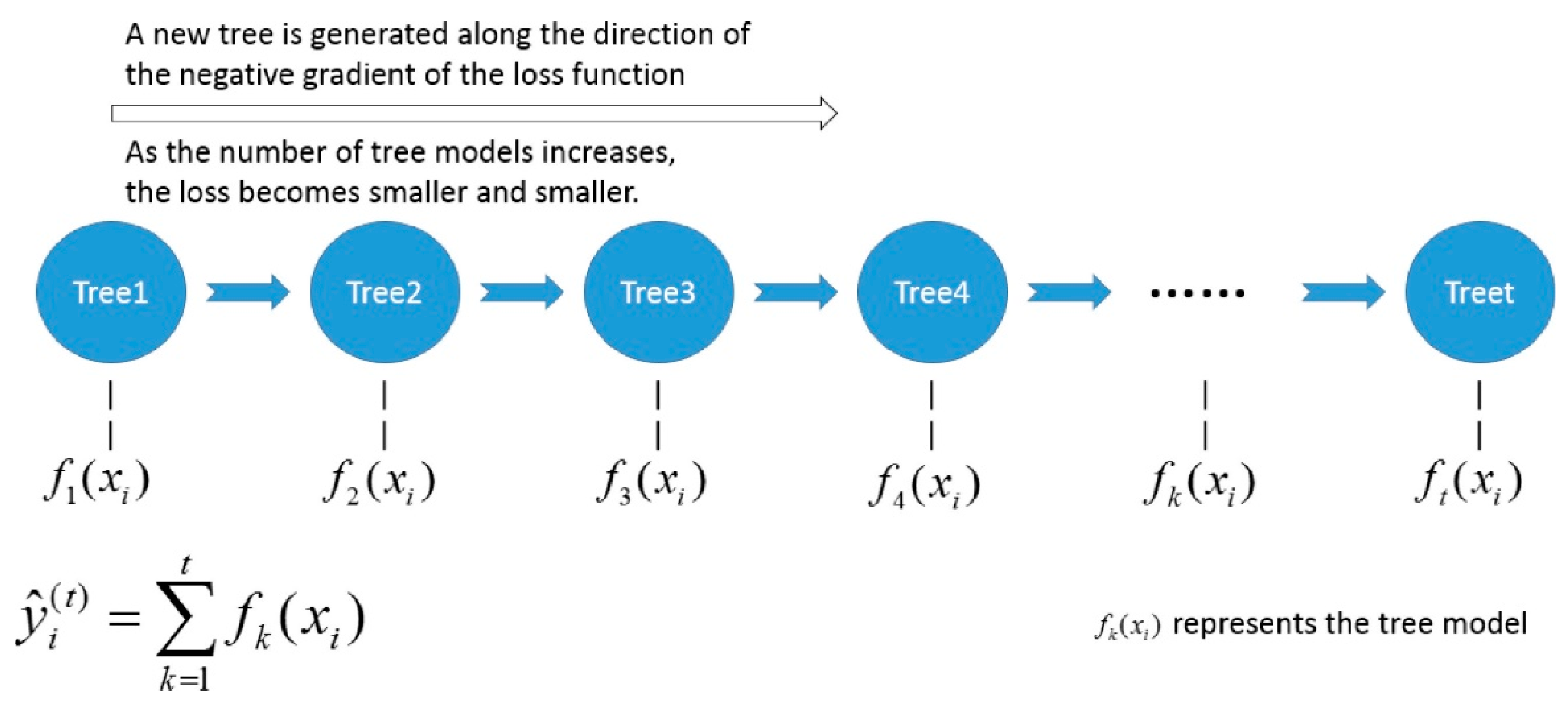
3.1. XGBoost
| Algorithm 1:Exact Greedy Algorithm for Split Finding. |
| Input:, instance set of the current node |
| Input:, feature dimension |
| for to do |
| for do |
| end |
| end |
| Output: Split with max score |
3.2. KPCA-LDA-XGB
4. Results and Discussion
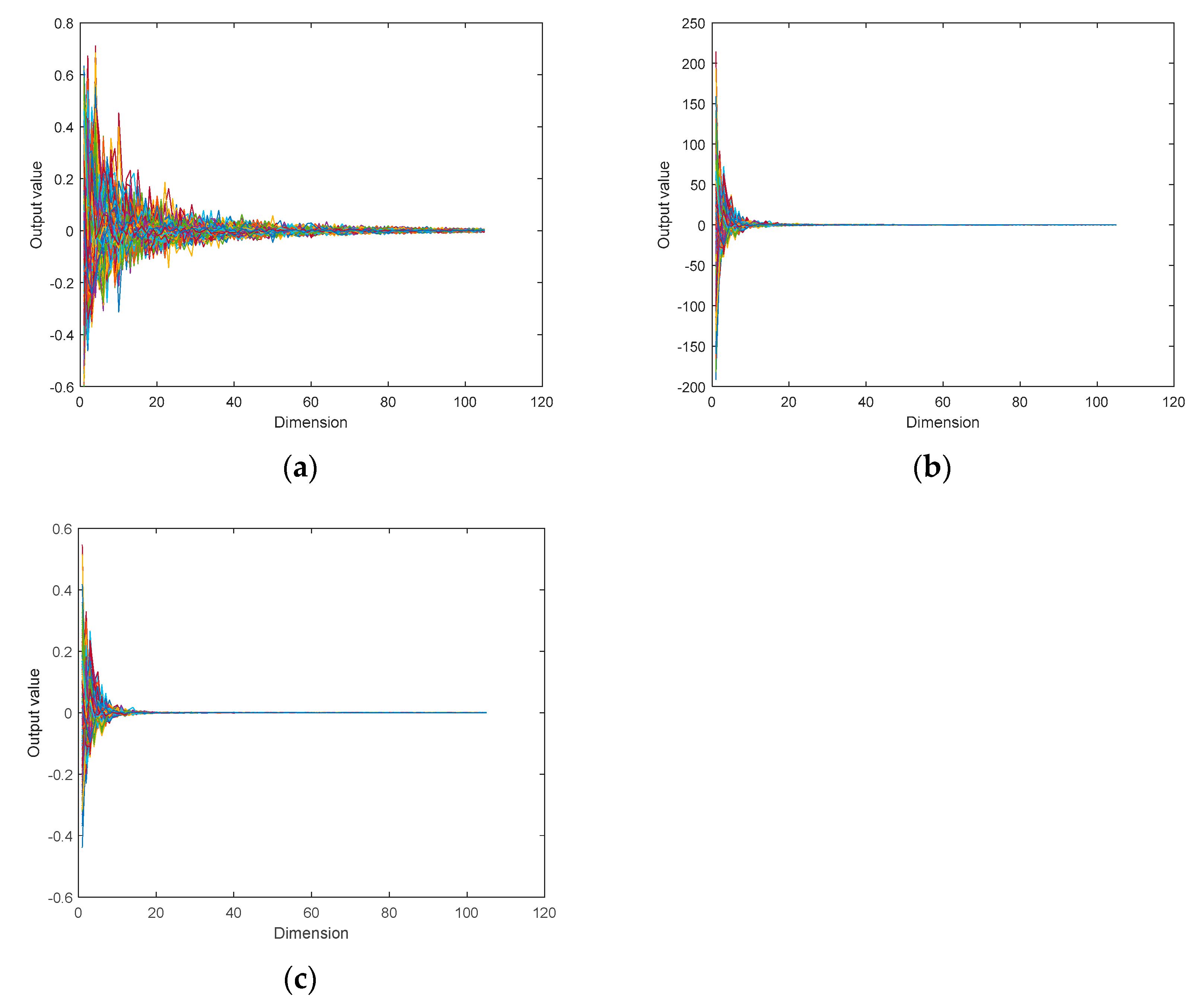
4.1. Performance Analysis of Different Kernel Functions
4.2. Performance Analysis of the KPCA-LDA-XGB Model
5. Conclusions
Author Contributions
Funding
Institutional Review Board Statement
Informed Consent Statement
Data Availability Statement
Acknowledgments
Conflicts of Interest
References
- Ni, C.; Wang, D.; Tao, Y. Variable weighted convolutional neural network for the nitrogen content quantization of Masson pine seedling leaves with near-infrared spectroscopy. Spectrochim. Acta Part A Mol. Biomol. Spectrosc. 2019, 209, 32–39. [Google Scholar] [CrossRef]
- Huang, Y.; Lu, R.; Chen, K. Detection of internal defect of apples by a multichannel Vis/NIR spectroscopic system. Postharvest Biol. Technol. 2020, 161, 111065. [Google Scholar] [CrossRef]
- Garrido-Novell, C.; Garrido-Varo, A.; Perez-Marin, D.; Guerrero-Ginel, J.E.; Kim, M. Quantification and spatial characteriza-tion of moisture and nacl content of iberian dry-cured ham slices using nir hyperspectral imaging. J. Food Eng. 2015, 153, 117–123. [Google Scholar] [CrossRef]
- Forchetti, D.A.; Poppi, R.J. Use of nir hyperspectral imaging and multivariate curve resolution (mcr) for detection and quantification of adulterants in milk powder. Lwt Food Sci. Technol. 2017, 76, 337–343. [Google Scholar] [CrossRef]
- Ni, C.; Li, Z.; Zhang, X.; Sun, X.; Huang, Y.; Zhao, L.; Zhu, T.; Wang, D. Online Sorting of the Film on Cotton Based on Deep Learning and Hyperspectral Imaging. IEEE Access 2020, 8, 93028–93038. [Google Scholar] [CrossRef]
- Dong, J.; Guo, W. Nondestructive Determination of Apple Internal Qualities Using Near-Infrared Hyperspectral Reflectance Imaging. Food Anal. Methods 2015, 8, 2635–2646. [Google Scholar] [CrossRef]
- Yuan, L.-M.; Sun, L.; Cai, J.; Lin, H. A Preliminary Study on Whether the Soluble Solid Content and Acidity of Oranges Predicted by Near Infrared Spectroscopy Meet the Sensory Degustation. J. Food Process. Eng. 2015, 38, 309–319. [Google Scholar] [CrossRef]
- Wei, X.; Liu, F.; Qiu, Z.; Shao, Y.; He, Y. Ripeness classification of astringent persimmon using hyperspectral imaging tech-nique. Food Bioprocess Technol. 2014, 7, 1371–1380. [Google Scholar] [CrossRef]
- Ciccoritti, R.; Paliotta, M.; Amoriello, T.; Carbone, K. FT-NIR spectroscopy and multivariate classification strategies for the postharvest quality of green-fleshed kiwifruit varieties. Sci. Hortic. 2019, 257. [Google Scholar] [CrossRef]
- Ali, A.M.; Darvishzadeh, R.; Skidmore, A.; Gara, T.W.; O’Connor, B.; Roeoesli, C.; Heurich, M.; Paganini, M. Comparing methods for mapping canopy chlorophyll content in a mixed mountain forest using Sentinel-2 data. Int. J. Appl. Earth Obs. Geoinf. 2020, 87, 102037. [Google Scholar] [CrossRef]
- Ainiwaer, M.; Ding, J.; Kasim, N.; Wang, J.; Wang, J. Regional scale soil moisture content estimation based on multi-source remote sensing parameters. Int. J. Remote Sens. 2019, 41, 3346–3367. [Google Scholar] [CrossRef]
- Huang, Y.; Lu, R.; Qi, C.; Chen, K. Measurement of Tomato Quality Attributes Based on Wavelength Ratio and Near-Infrared Spectroscopy. Spectrosc. Spectr. Anal. 2018, 38, 2362–2368. [Google Scholar]
- Shen, L.; Wang, H.; Liu, Y.; Liu, Y.; Zhang, X.; Fei, Y. Prediction of Soluble Solids Content in Green Plum by Using a Sparse Autoencoder. Appl. Sci. 2020, 10, 3769. [Google Scholar] [CrossRef]
- Dissanayake, T.; Rajapaksha, Y.; Ragel, R.; Nawinne, I. An Ensemble Learning Approach for Electrocardiogram Sensor Based Human Emotion Recognition. Sensors 2019, 19, 4495. [Google Scholar] [CrossRef]
- Zhu, C.; Zhang, Z.; Wang, H.; Wang, J.; Yang, S. Assessing Soil Organic Matter Content in a Coal Mining Area through Spectral Variables of Different Numbers of Dimensions. Sensors 2020, 20, 1795. [Google Scholar] [CrossRef]
- Li, S.; Jia, M.; Dong, D. Fast Measurement of Sugar in Fruits Using Near Infrared Spectroscopy Combined with Random Forest Algorithm. Spectrosc. Spectr. Anal. 2018, 38, 1766–1771. [Google Scholar]
- Chen, T.; Guestrin, C. XGBoost: A Scalable Tree Boosting System. In Proceedings of the 22nd ACM SIGKDD International Con-ference on Knowledge Discovery and Data Mining, San Francisco, CA, USA, 13–17 August 2016; ACM: New York, NY, USA, 2016; pp. 785–794. [Google Scholar]
- Zopluoglu, C. Detecting Examinees with Item Preknowledge in Large-Scale Testing Using Extreme Gradient Boosting (XGBoost). Educ. Psychol. Meas. 2019, 7, 931–961. [Google Scholar] [CrossRef]
- Zhang, X.; Luo, A. XGBoost based stellar spectral classification and quantized feature. Spectrosc. Spectr. Anal. 2019, 39, 3292–3296. [Google Scholar]
- Mo, H.; Sun, H.; Liu, J.; Wei, S. Developing window behavior models for residential buildings using XGBoost algorithm. Energy Build. 2019, 205, 109564. [Google Scholar] [CrossRef]
- Huang, J.; Yan, X. Quality Relevant and Independent Two Block Monitoring Based on Mutual Information and KPCA. IEEE Trans. Ind. Electron. 2017, 64, 6518–6527. [Google Scholar] [CrossRef]
- Walsh, K.B.; José, B.; Zude-Sasse, M.; Sun, X. Visible-NIR ’point’ spectroscopy in postharvest fruit and vegetable assessment: The science behind three decades of commercial use. Postharvest Biol. Technol. 2020, 168, 111246. [Google Scholar] [CrossRef]


| Specifications | Parameters |
|---|---|
| Spectral range | 400–1000 nm |
| Spectral resolution | 2.8 nm |
| Data output | 16 bits |
| Data interface | USB3.0/CameraLink |
| Sample Set | n | Max | Min | Mean | SD |
|---|---|---|---|---|---|
| Calibration set | 274 | 2.74 | 2.03 | 2.26 | 0.1399 |
| Prediction set | 92 | 2.71 | 2.04 | 2.27 | 0.1327 |
| Name | Parameter |
|---|---|
| System | Windows 10 × 64 |
| CPU | Inter I9 9900K@3.60 GHz |
| GPU | Nvidia GeForce RTX 2080 Ti(11G) |
| Environment configuration | PyCharm + Tensorflow 2.1.0 + Python 3.7.7 Cuda 10.0 + cudnn 7.6.5 + XGBoost 1.1.1 |
| RAM | 64 GB |
| Model | RP | RMSEP | RCV | RMSECV |
|---|---|---|---|---|
| KPCA(RBF)-LDA-XGB | 0.805 | 0.112 | 0.744 | 0.128 |
| KPCA(Poly)-LDA-XGB | 0.814 | 0.108 | 0.753 | 0.126 |
| KPCA(linear)-LDA-XGB | 0.829 | 0.107 | 0.739 | 0.128 |
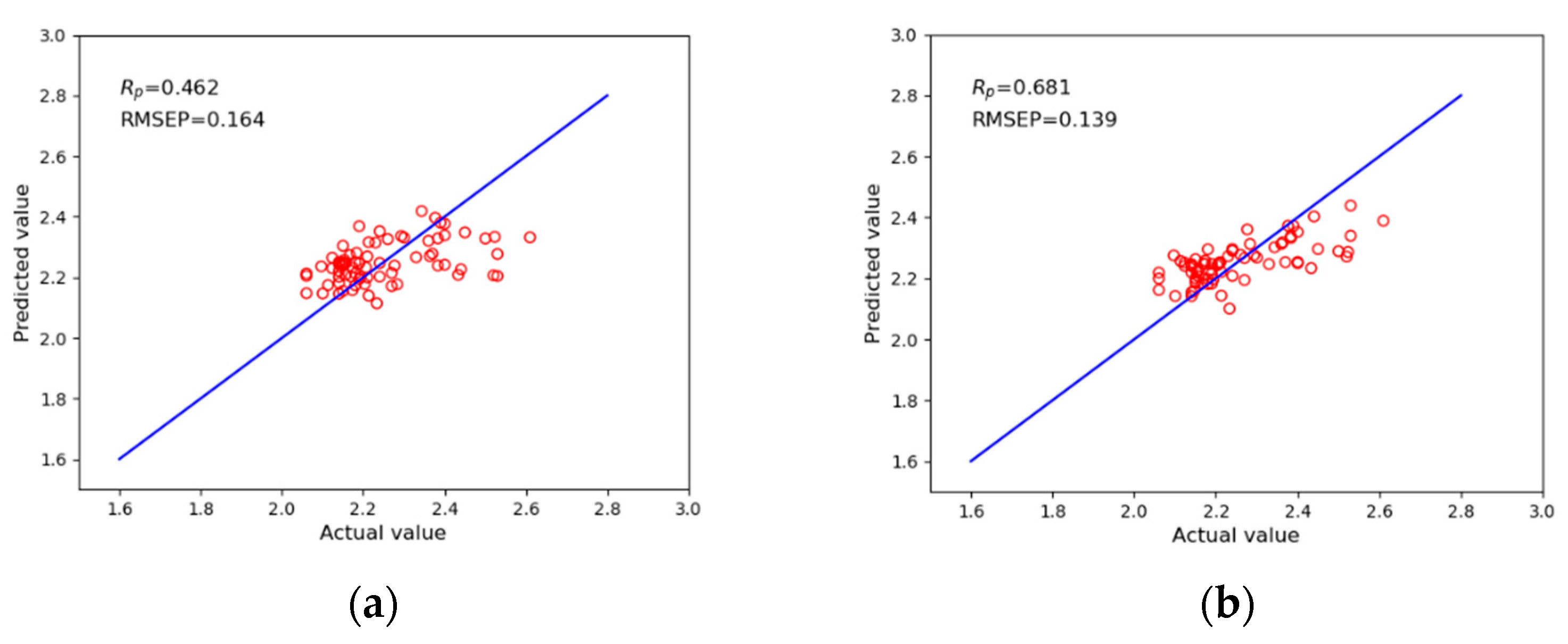
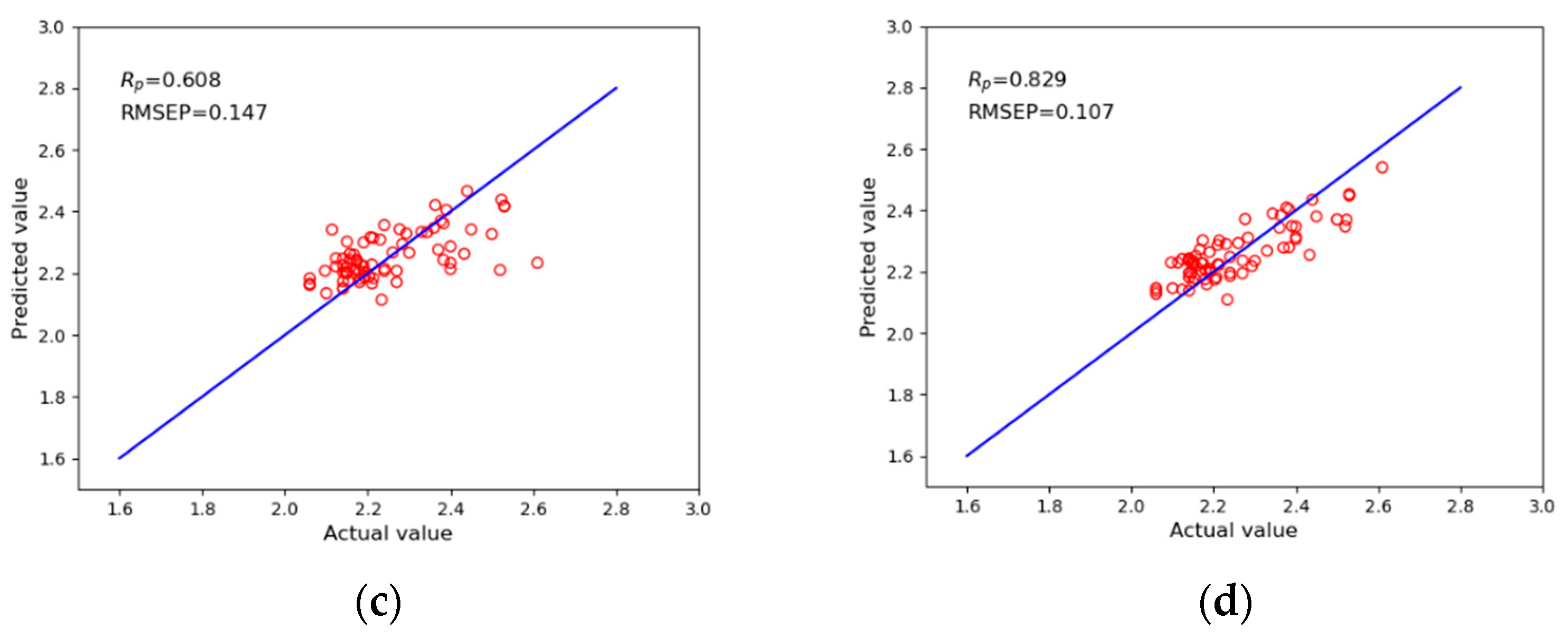
| Model | RP | RMSEP | RCV | RMSECV |
|---|---|---|---|---|
| XGBoost | 0.462 | 0.164 | 0.214 | 0.186 |
| KPCA-XGB | 0.681 | 0.139 | 0.589 | 0.155 |
| LDA-XGB | 0.608 | 0.147 | 0.655 | 0.144 |
| KPCA-LDA-XGB | 0.829 | 0.107 | 0.739 | 0.128 |
Publisher’s Note: MDPI stays neutral with regard to jurisdictional claims in published maps and institutional affiliations. |
© 2021 by the authors. Licensee MDPI, Basel, Switzerland. This article is an open access article distributed under the terms and conditions of the Creative Commons Attribution (CC BY) license (http://creativecommons.org/licenses/by/4.0/).
Share and Cite
Liu, Y.; Wang, H.; Fei, Y.; Liu, Y.; Shen, L.; Zhuang, Z.; Zhang, X. Research on the Prediction of Green Plum Acidity Based on Improved XGBoost. Sensors 2021, 21, 930. https://doi.org/10.3390/s21030930
Liu Y, Wang H, Fei Y, Liu Y, Shen L, Zhuang Z, Zhang X. Research on the Prediction of Green Plum Acidity Based on Improved XGBoost. Sensors. 2021; 21(3):930. https://doi.org/10.3390/s21030930
Chicago/Turabian StyleLiu, Yang, Honghong Wang, Yeqi Fei, Ying Liu, Luxiang Shen, Zilong Zhuang, and Xiao Zhang. 2021. "Research on the Prediction of Green Plum Acidity Based on Improved XGBoost" Sensors 21, no. 3: 930. https://doi.org/10.3390/s21030930
APA StyleLiu, Y., Wang, H., Fei, Y., Liu, Y., Shen, L., Zhuang, Z., & Zhang, X. (2021). Research on the Prediction of Green Plum Acidity Based on Improved XGBoost. Sensors, 21(3), 930. https://doi.org/10.3390/s21030930