
Complex Pignistic Transformation-Based Evidential Distance for Multisource Information Fusion of Medical Diagnosis in the IoT


Abstract
1. Introduction
- This is the first work to propose the complex pignistic transformation-based evidential betting commitment distance (BCD) for the multisource information fusion of medical diagnosis in the IoT.
- The BCD is a strict distance metric that satisfies the axioms of the nonnegativity, nondegeneracy, symmetry, and triangle inequality, which is a generalization of the classical evidential distance of Liu.
- A basis algorithm and its weighted extension for decision-making are designed on the basis of the BCD, which are applied to the medical IoT to demonstrate their effectiveness.
2. Preliminaries
2.1. Medical IoT
2.2. Uncertainty Modeling and Information Fusion
2.3. Complex Evidence Theory
2.4. Versus Conflict
3. A New Conflict Measure Model
3.1. Complex Pignistic Transformation
3.2. Betting Commitment-Based Distance Versus Conflict
4. Comparisons and Analysis
- R 1:
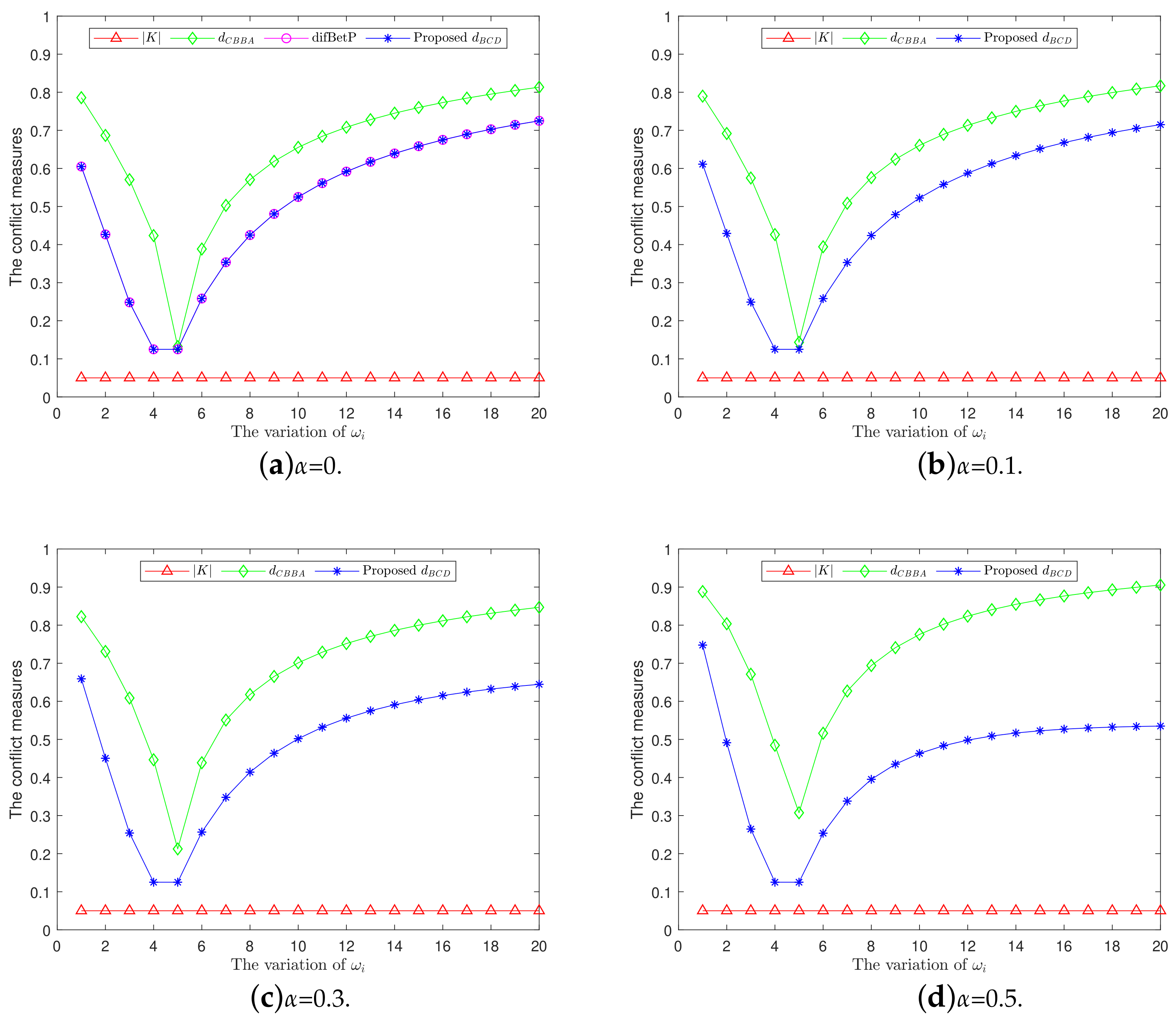
- For , it can be seen that it can measure well the conflict between CBBAs in Case 1 and Case 2 with values of 0.84 and 0.264, respectively. However, cannot distinguish the difference among the CBBAs in Case 3 with a measure value of zero.
- R 2:
- For , it is obvious that can measure the conflicts among the CBBAs in Case 1, Case 2, and Case 3 with values of 0.7071, 0.5802, and 0.7242, respectively. Comparing the conflict value of 0.7071 between and and 0.7242 between and , it is noticed that the result of is not up to our expectations.
- R 3:
- For , it is easy to see that can well measure the conflicts among the CBBAs in all three cases with values of 0.7062, 0.4380, and 0.6062, respectively. Comparing the conflict value of 0.7062 of with 0.6062 of , it is obtained that . This result satisfies our expectation.
- R 4:
- It is concluded that the BCD is a better conflict measure compared with the methods of and to judge the contradiction among CBBAs.
5. Algorithm and Application
5.1. Algorithm for Decision-Making
- Step 1:
- The BCD is used to calculate the distance between and :
- Step 2:
- The minimal distance between and is elected:
- Step 3:
- is sorted into pattern by:
| Algorithm 1: Multi-attribute decision-making. |
 |
5.2. Application in Medical Diagnosis Under the Smart IoT Environment
- Step 1:
- The BCDs between and , and , and and are calculated:
- Step 2:
- The minimal BCD is :
- Step 3:
- is determined to be the most likely to suffer from the disease type of :
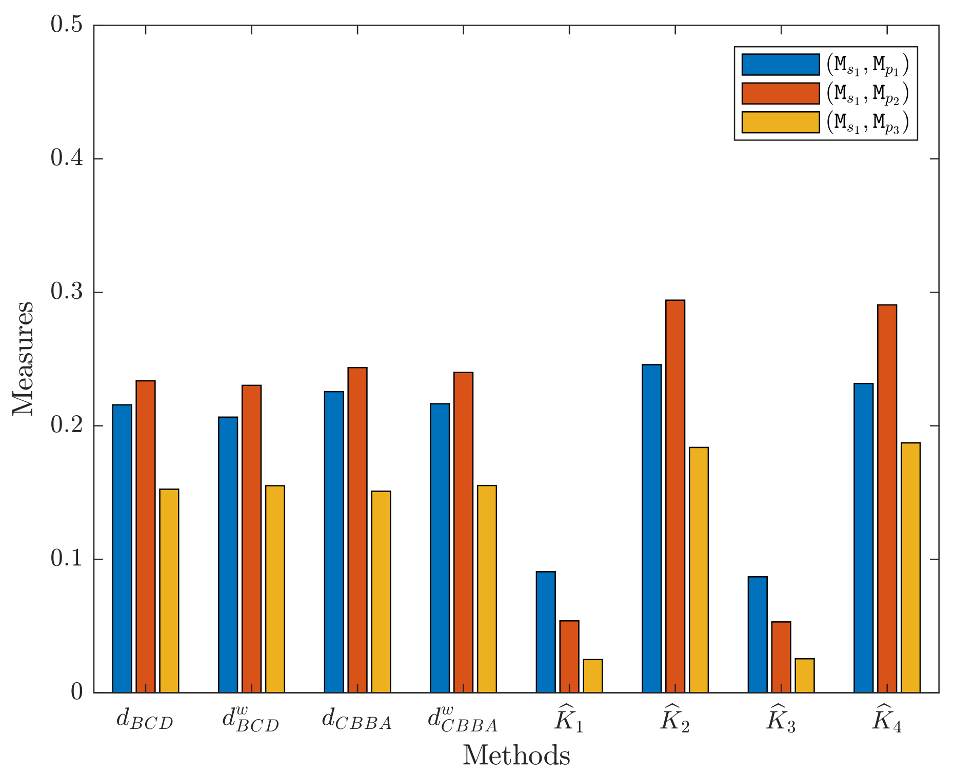
5.3. Extension and Comparison
6. Conclusions
Funding
Acknowledgments
Conflicts of Interest
References
- Qi, J.; Yang, P.; Newcombe, L.; Peng, X.; Yang, Y.; Zhao, Z. An overview of data fusion techniques for Internet of Things enabled physical activity recognition and measure. Inf. Fusion 2020, 55, 269–280. [Google Scholar] [CrossRef]
- Huang, K.; Zhang, Q.; Zhou, C.; Xiong, N.; Qin, Y. An efficient intrusion detection approach for visual sensor networks based on traffic pattern learning. IEEE Trans. Syst. Man Cybern. Syst. 2017, 47, 2704–2713. [Google Scholar] [CrossRef]
- Alabdulkarim, A.; Al-Rodhaan, M.; Ma, T.; Tian, Y. PPSDT: A novel privacy-preserving single decision tree algorithm for clinical decision-support systems using IoT devices. Sensors 2019, 19, 142. [Google Scholar] [CrossRef] [PubMed]
- Roy, M.; Chowdhury, C.; Aslam, N. Designing transmission strategies for enhancing communications in medical IoT using Markov decision process. Sensors 2018, 18, 4450. [Google Scholar] [CrossRef] [PubMed]
- Souza, L.F.D.F.; Silva, I.C.L.; Marques, A.G.; Silva, F.H.D.S.; Nunes, V.X.; Hassan, M.M.; Albuquerque, V.H.C.D. Internet of Medical Things: An Effective and Fully Automatic IoT Approach Using Deep Learning and Fine-Tuning to Lung CT Segmentation. Sensors 2020, 20, 6711. [Google Scholar] [CrossRef] [PubMed]
- Celesti, A.; Ruggeri, A.; Fazio, M.; Galletta, A.; Villari, M.; Romano, A. Blockchain-Based Healthcare Workflow for Tele-Medical Laboratory in Federated Hospital IoT Clouds. Sensors 2020, 20, 2590. [Google Scholar] [CrossRef] [PubMed]
- Takabayashi, K.; Tanaka, H.; Sakakibara, K. Integrated Performance Evaluation of the Smart Body Area Networks Physical Layer for Future Medical and Healthcare IoT. Sensors 2019, 19, 30. [Google Scholar] [CrossRef]
- Mavrogiorgou, A.; Kiourtis, A.; Perakis, K.; Pitsios, S.; Kyriazis, D. IoT in healthcare: Achieving interoperability of high-quality data acquired by IoT medical devices. Sensors 2019, 19, 1978. [Google Scholar] [CrossRef]
- Depari, A.; Fernandes Carvalho, D.; Bellagente, P.; Ferrari, P.; Sisinni, E.; Flammini, A.; Padovani, A. An IoT based architecture for enhancing the effectiveness of prototype medical instruments applied to neurodegenerative disease diagnosis. Sensors 2019, 19, 1564. [Google Scholar] [CrossRef]
- Dempster, A.P. Upper and Lower Probabilities Induced by a Multivalued Mapping. Ann. Math. Stat. 1967, 38, 325–339. [Google Scholar] [CrossRef]
- Shafer, G. A Mathematical Theory of Evidence; Princeton University Press: Princeton, NJ, USA, 1976; Volume 1. [Google Scholar]
- Deng, Y. Information volume of mass function. Int. J. Comput. Commun. Control 2020, 15, 3983. [Google Scholar] [CrossRef]
- Xiao, F. EFMCDM: Evidential fuzzy multicriteria decision making based on belief entropy. IEEE Trans. Fuzzy Syst. 2020, 28, 1477–1491. [Google Scholar] [CrossRef]
- Zhou, M.; Liu, X.B.; Chen, Y.W.; Yang, J.B. Evidential reasoning rule for MADM with both weights and reliabilities in group decision making. Knowl.-Based Syst. 2018, 143, 142–161. [Google Scholar] [CrossRef]
- Pan, L.; Deng, Y. Probability transform based on the ordered weighted averaging and entropy difference. Int. J. Comput. Commun. Control 2020, 15, 3743. [Google Scholar] [CrossRef]
- Yager, R.R. Generalized Dempster–Shafer Structures. IEEE Trans. Fuzzy Syst. 2019, 27, 428–435. [Google Scholar] [CrossRef]
- Song, Y.; Zhu, J.; Lei, L.; Wang, X. A Self-adaptive combination method for temporal evidence based on negotiation strategy. SCIENCE CHINA Inf. Sci. 2020, 63, 210204. [Google Scholar] [CrossRef]
- Deng, X.; Jiang, W. Evaluating green supply chain management practices under fuzzy environment: A novel method based on D number theory. Int. J. Fuzzy Syst. 2019, 21, 1389–1402. [Google Scholar] [CrossRef]
- Deng, X.; Jiang, W. A total uncertainty measure for D numbers based on belief intervals. Int. J. Intell. Syst. 2019, 34, 3302–3316. [Google Scholar] [CrossRef]
- Yang, J.B.; Xu, D.L. Evidential reasoning rule for evidence combination. Artif. Intell. 2013, 205, 1–29. [Google Scholar] [CrossRef]
- Fujita, H.; Ko, Y.C. A heuristic representation learning based on evidential memberships: Case study of UCI-SPECTF. Int. J. Approx. Reason. 2020, 120, 125–137. [Google Scholar] [CrossRef]
- Deng, Y. Uncertainty measure in evidence theory. Sci. China Inf. Sci. 2020, 63, 210201. [Google Scholar] [CrossRef]
- Deng, Y. Deng entropy measure of quantum entanglement. chinaXiv 2021. [Google Scholar]
- Fan, L.; Deng, Y. Determine the number of unknown targets in Open World based on Elbow method. IEEE Trans. Fuzzy Syst. 2020, 1. [Google Scholar] [CrossRef]
- Li, Y.X.; Pelusi, D.; Deng, Y. Generate two dimensional belief function based on an improved similarity measure of trapezoidal fuzzy numbers. Comput. Appl. Math. 2020, 39, 1–20. [Google Scholar] [CrossRef]
- Mao, S.; Han, Y.; Deng, Y.; Pelusi, D. A hybrid DEMATEL-FRACTAL method of handling dependent evidences. Eng. Appl. Artif. Intell. 2020, 91, 103543. [Google Scholar] [CrossRef]
- Luo, Z.; Deng, Y. A matrix method of basic belief assignment’s negation in Dempster–Shafer theory. IEEE Trans. Fuzzy Syst. 2020, 28, 2270–2276. [Google Scholar] [CrossRef]
- Xiao, F. Generalization of Dempster–Shafer theory: A complex mass function. Appl. Intell. 2020, 50, 3266–3275. [Google Scholar] [CrossRef]
- Xiao, F. Generalized belief function in complex evidence theory. J. Intell. Fuzzy Syst. 2020, 38, 3665–3673. [Google Scholar] [CrossRef]
- Garg, H.; Rani, D. A robust correlation coefficient measure of complex intuitionistic fuzzy sets and their applications in decision-making. Appl. Intell. 2019, 49, 496–512. [Google Scholar] [CrossRef]
- Han, D.; Dezert, J.; Yang, Y. Belief interval-based distance measures in the theory of belief functions. IEEE Trans. Syst. Man Cybern. Syst. 2016, 48, 833–850. [Google Scholar] [CrossRef]
- Yang, Y.; Han, D. A new distance-based total uncertainty measure in the theory of belief functions. Knowl.-Based Syst. 2016, 94, 114–123. [Google Scholar] [CrossRef]
- Jousselme, A.L.; Grenier, D.; Bossé, É. A new distance between two bodies of evidence. Inf. Fusion 2001, 2, 91–101. [Google Scholar] [CrossRef]
- Jousselme, A.L.; Maupin, P. Distances in evidence theory: Comprehensive survey and generalizations. Int. J. Approx. Reason. 2012, 53, 118–145. [Google Scholar] [CrossRef]
- Bouchard, M.; Jousselme, A.L.; Doré, P.E. A proof for the positive definiteness of the Jaccard index matrix. Int. J. Approx. Reason. 2013, 54, 615–626. [Google Scholar] [CrossRef]
- Jiang, W.; Huang, C.; Deng, X. A new probability transformation method based on a correlation coefficient of belief functions. Int. J. Intell. Syst. 2019, 34, 1337–1347. [Google Scholar] [CrossRef]
- Xiao, F.; Cao, Z.; Jolfaei, A. A novel conflict measurement in decision making and its application in fault diagnosis. IEEE Trans. Fuzzy Syst. 2020, 29, 186–197. [Google Scholar] [CrossRef]
- Pan, L.; Deng, Y. An association coefficient of belief function and its application in target recognition system. Int. J. Intell. Syst. 2020, 35, 85–104. [Google Scholar] [CrossRef]
- Liu, W. Analyzing the degree of conflict among belief functions. Artif. Intell. 2006, 170, 909–924. [Google Scholar] [CrossRef]
- Xiao, F. CED: A distance for complex mass functions. IEEE Trans. Neural Netw. Learn. Syst. 2020, 1. [Google Scholar] [CrossRef]
- Huang, J.; Wu, X.; Huang, W.; Wu, X.; Wang, S. Internet of things in health management systems: A review. Int. J. Commun. Syst. 2020, e4683. [Google Scholar] [CrossRef]
- Hossain, M.S.; Muhammad, G. Cloud-assisted industrial Internet of Things (IIoT)–enabled framework for health monitoring. Comput. Netw. 2016, 101, 192–202. [Google Scholar] [CrossRef]
- Gómez, J.; Oviedo, B.; Zhuma, E. Patient monitoring system based on Internet of Things. Procedia Comput. Sci. 2016, 83, 90–97. [Google Scholar] [CrossRef]
- Abawajy, J.H.; Hassan, M.M. Federated internet of things and cloud computing pervasive patient health monitoring system. IEEE Commun. Mag. 2017, 55, 48–53. [Google Scholar] [CrossRef]
- He, D.; Zeadally, S. An analysis of RFID authentication schemes for internet of things in healthcare environment using elliptic curve cryptography. IEEE Internet Things J. 2014, 2, 72–83. [Google Scholar] [CrossRef]
- Dimitrov, D.V. Medical internet of things and big data in healthcare. Healthc. Inform. Res. 2016, 22, 156–163. [Google Scholar] [CrossRef]
- Lomotey, R.K.; Pry, J.; Sriramoju, S. Wearable IoT data stream traceability in a distributed health information system. Pervasive Mob. Comput. 2017, 40, 692–707. [Google Scholar] [CrossRef]
- Zhang, W.; Yang, J.; Su, H.; Kumar, M.; Mao, Y. Medical data fusion algorithm based on Internet of Things. Pers. Ubiquitous Comput. 2018, 22, 895–902. [Google Scholar] [CrossRef]
- Dautov, R.; Distefano, S.; Buyya, R. Hierarchical data fusion for Smart Healthcare. J. Big Data 2019, 6, 19. [Google Scholar] [CrossRef]
- Xiao, F. Evidence combination based on prospect theory for multi-sensor data fusion. ISA Trans. 2020, 106, 253–261. [Google Scholar] [CrossRef]
- Meng, D.; Liu, M.; Yang, S.; Zhang, H.; Ding, R. A fluid–structure analysis approach and its application in the uncertainty-based multidisciplinary design and optimization for blades. Adv. Mech. Eng. 2018, 10. [Google Scholar] [CrossRef]
- Liu, Z.; Li, G.; Mercier, G.; He, Y.; Pan, Q. Change detection in heterogenous remote sensing images via homogeneous pixel transformation. IEEE Trans. Image Process. 2017, 27, 1822–1834. [Google Scholar] [CrossRef] [PubMed]
- Yager, R.R. On Using the Shapley Value to Approximate the Choquet Integral in Cases of Uncertain Arguments. IEEE Trans. Fuzzy Syst. 2018, 26, 1303–1310. [Google Scholar] [CrossRef]
- Gao, X.; Deng, Y. The pseudo-pascal triangle of maximum Deng entropy. Int. J. Comput. Commun. Control 2020, 15, 1006. [Google Scholar] [CrossRef]
- Li, Y.F.; Huang, H.Z.; Mi, J.; Peng, W.; Han, X. Reliability analysis of multi-state systems with common cause failures based on Bayesian network and fuzzy probability. Ann. Oper. Res. 2019, 1–15. [Google Scholar] [CrossRef]
- Feng, F.; Cho, J.; Pedrycz, W.; Fujita, H.; Herawan, T. Soft set based association rule mining. Knowl.-Based Syst. 2016, 111, 268–282. [Google Scholar] [CrossRef]
- Witarsyah, D.; Fudzee, M.F.M.; Salamat, M.A.; Yanto, I.T.R.; Abawajy, J. Soft Set Theory Based Decision Support System for Mining Electronic Government Dataset. Int. J. Data Warehous. Min. (IJDWM) 2020, 16, 39–62. [Google Scholar] [CrossRef]
- Haruna, K.; Ismail, M.A.; Suyanto, M.; Gabralla, L.A.; Bichi, A.B.; Danjuma, S.; Kakudi, H.A.; Haruna, M.S.; Zerdoumi, S.; Abawajy, J.H.; et al. A soft set approach for handling conflict situation on movie selection. IEEE Access 2019, 7, 116179–116194. [Google Scholar] [CrossRef]
- Yang, J.; Li, S.; Xu, Z.; Liu, H.; Yao, W. An understandable way to extend the ordinary linear order on real numbers to a linear order on interval numbers. IEEE Trans. Fuzzy Syst. 2020, 1. [Google Scholar] [CrossRef]
- Fei, L.; Feng, Y.; Liu, L. Evidence combination using OWA-based soft likelihood functions. Int. J. Intell. Syst. 2019, 34, 2269–2290. [Google Scholar] [CrossRef]
- Jiang, W.; Cao, Y.; Deng, X. A novel Z-network model based on Bayesian network and Z-number. IEEE Trans. Fuzzy Syst. 2020, 28, 1585–1599. [Google Scholar] [CrossRef]
- Tian, Y.; Liu, L.; Mi, X.; Kang, B. ZSLF: A new soft likelihood function based on Z-numbers and its application in expert decision system. IEEE Trans. Fuzzy Syst. 2020, 1–11. [Google Scholar] [CrossRef]
- Xiao, F. On the maximum entropy negation of a complex-valued distribution. IEEE Trans. Fuzzy Syst. 2020, 1–11. [Google Scholar] [CrossRef]
- Xiao, F. GIQ: A generalized intelligent quality-based approach for fusing multi-source information. IEEE Trans. Fuzzy Syst. 2020, 1–11. [Google Scholar] [CrossRef]
- Garg, H.; Rani, D. Some results on information measures for complex intuitionistic fuzzy sets. Int. J. Intell. Syst. 2019, 34, 2319–2363. [Google Scholar] [CrossRef]
- Lai, J.W.; Cheong, K.H. Parrondo’s paradox from classical to quantum: A review. Nonlinear Dyn. 2020, 100, 1–13. [Google Scholar] [CrossRef]
- Gao, X.; Deng, Y. Quantum model of mass function. Int. J. Intell. Syst. 2020, 35, 267–282. [Google Scholar] [CrossRef]
- Jiang, W.; Huang, K.; Geng, J.; Deng, X. Multi-Scale Metric Learning for Few-Shot Learning. IEEE Trans. Circuits Syst. Video Technol. 2020, 1. [Google Scholar] [CrossRef]
- Deng, J.; Deng, Y. Information volume of fuzzy membership function. Int. J. Comput. Commun. Control 2021, 16, 4106. [Google Scholar] [CrossRef]
- Tang, M.; Liao, H.; Herrera-Viedma, E.; Chen, C.P.; Pedrycz, W. A Dynamic Adaptive Subgroup-to-Subgroup Compatibility-Based Conflict Detection and Resolution Model for Multicriteria Large-Scale Group Decision Making. IEEE Trans. Cybern. 2020, 1–12. [Google Scholar] [CrossRef]
- Cao, Z.; Chuang, C.H.; King, J.K.; Lin, C.T. Multi-channel EEG recordings during a sustained-attention driving task. Sci. Data 2019, 6, 1–8. [Google Scholar] [CrossRef]
- Liu, P.; Zhang, X. A new hesitant fuzzy linguistic approach for multiple attribute decision making based on Dempster–Shafer evidence theory. Appl. Soft Comput. 2020, 86, 105897. [Google Scholar] [CrossRef]
- Liu, Q.; Tian, Y.; Kang, B. Derive knowledge of Z-number from the perspective of Dempster–Shafer evidence theory. Eng. Appl. Artif. Intell. 2019, 85, 754–764. [Google Scholar] [CrossRef]
- Xu, X.; Zheng, J.; Yang, J.b.; Xu, D.l.; Chen, Y.w. Data classification using evidence reasoning rule. Knowl.-Based Syst. 2017, 116, 144–151. [Google Scholar] [CrossRef]
- Pan, Y.; Zhang, L.; Wu, X.; Skibniewski, M.J. Multi-classifier information fusion in risk analysis. Inf. Fusion 2020, 60, 121–136. [Google Scholar] [CrossRef]
- Fu, C.; Chang, W.; Yang, S. Multiple criteria group decision making based on group satisfaction. Inf. Sci. 2020, 518, 309–329. [Google Scholar] [CrossRef]
- Fei, L.; Lu, J.; Feng, Y. An extended best-worst multi-criteria decision-making method by belief functions and its applications in hospital service evaluation. Comput. Ind. Eng. 2020, 142, 106355. [Google Scholar] [CrossRef]
- Kang, B.; Zhang, P.; Gao, Z.; Chhipi-Shrestha, G.; Hewage, K.; Sadiq, R. Environmental assessment under uncertainty using Dempster–Shafer theory and Z-numbers. J. Ambient Intell. Humaniz. Comput. 2020, 11, 2041–2060. [Google Scholar] [CrossRef]
- Liu, Z.; Pan, Q.; Dezert, J.; Han, J.W.; He, Y. Classifier fusion with contextual reliability evaluation. IEEE Trans. Cybern. 2018, 48, 1605–1618. [Google Scholar] [CrossRef]
- Xiao, F. CEQD: A complex mass function to predict interference effects. IEEE Trans. Cybern. 2020, 1–13. [Google Scholar] [CrossRef]
- Xiao, F. A distance measure for intuitionistic fuzzy sets and its application to pattern classification problems. IEEE Trans. Syst. Man Cybern. Syst. 2019, 1–13. [Google Scholar] [CrossRef]
- Fei, L.; Feng, Y.; Liu, L. On Pythagorean fuzzy decision making using soft likelihood functions. Int. J. Intell. Syst. 2019, 34, 3317–3335. [Google Scholar] [CrossRef]
- Xue, Y.; Deng, Y.; Garg, H. Uncertain database retrieval with measure-based belief function attribute values under intuitionistic fuzzy set. Inf. Sci. 2020, 546, 436–447. [Google Scholar] [CrossRef]


| i | |
|---|---|
| 1 | |
| 2 | |
| 3 | |
| 4 | |
| 5 | |
| 6 | |
| 7 | |
| 8 | |
| 9 | |
| 10 | |
| 11 | |
| 12 | |
| 13 | |
| 14 | |
| 15 | |
| 16 | |
| 17 | |
| 18 | |
| 19 | |
| 20 |
| Methods | Conflict Measures | ||
|---|---|---|---|
| Case 1: | Case 2: | Case 3: | |
| 0.8400 | 0.2640 | 0.0000 | |
| 0.7071 | 0.5802 | 0.7242 | |
| 0.7062 | 0.4380 | 0.6062 | |
| CBBAs | ||||
|---|---|---|---|---|
| 0 | ||||
| 0 | ||||
| 0 | ||||
| 0 | ||||
| 0 | ||||
| 0 | ||||
| 0 | ||||
| CBBAs | ||||
|---|---|---|---|---|
| Methods | Measures | ||
|---|---|---|---|
| 0.2157 | 0.2337 | 0.1525 | |
| 0.2065 | 0.2303 | 0.1551 | |
| 0.2256 | 0.2436 | 0.1526 | |
| 0.2165 | 0.2400 | 0.1553 | |
| 0.0907 | 0.0539 | 0.0249 | |
| 0.2458 | 0.2941 | 0.1838 | |
| 0.0869 | 0.0531 | 0.0255 | |
| 0.2317 | 0.2906 | 0.1872 | |
| Methods | Rankings | Sort |
|---|---|---|
Publisher’s Note: MDPI stays neutral with regard to jurisdictional claims in published maps and institutional affiliations. |
© 2021 by the author. Licensee MDPI, Basel, Switzerland. This article is an open access article distributed under the terms and conditions of the Creative Commons Attribution (CC BY) license (http://creativecommons.org/licenses/by/4.0/).
Share and Cite
Xiao, F. Complex Pignistic Transformation-Based Evidential Distance for Multisource Information Fusion of Medical Diagnosis in the IoT. Sensors 2021, 21, 840. https://doi.org/10.3390/s21030840
Xiao F. Complex Pignistic Transformation-Based Evidential Distance for Multisource Information Fusion of Medical Diagnosis in the IoT. Sensors. 2021; 21(3):840. https://doi.org/10.3390/s21030840
Chicago/Turabian StyleXiao, Fuyuan. 2021. "Complex Pignistic Transformation-Based Evidential Distance for Multisource Information Fusion of Medical Diagnosis in the IoT" Sensors 21, no. 3: 840. https://doi.org/10.3390/s21030840
APA StyleXiao, F. (2021). Complex Pignistic Transformation-Based Evidential Distance for Multisource Information Fusion of Medical Diagnosis in the IoT. Sensors, 21(3), 840. https://doi.org/10.3390/s21030840