Curve-Based Classification Approach for Hyperspectral Dermatologic Data Processing

 ,
,  ,
,  , ,
, , 
Abstract
:1. Introduction
2. Materials and Methods
2.1. Hyperspectral In Vivo Dermatologic Data
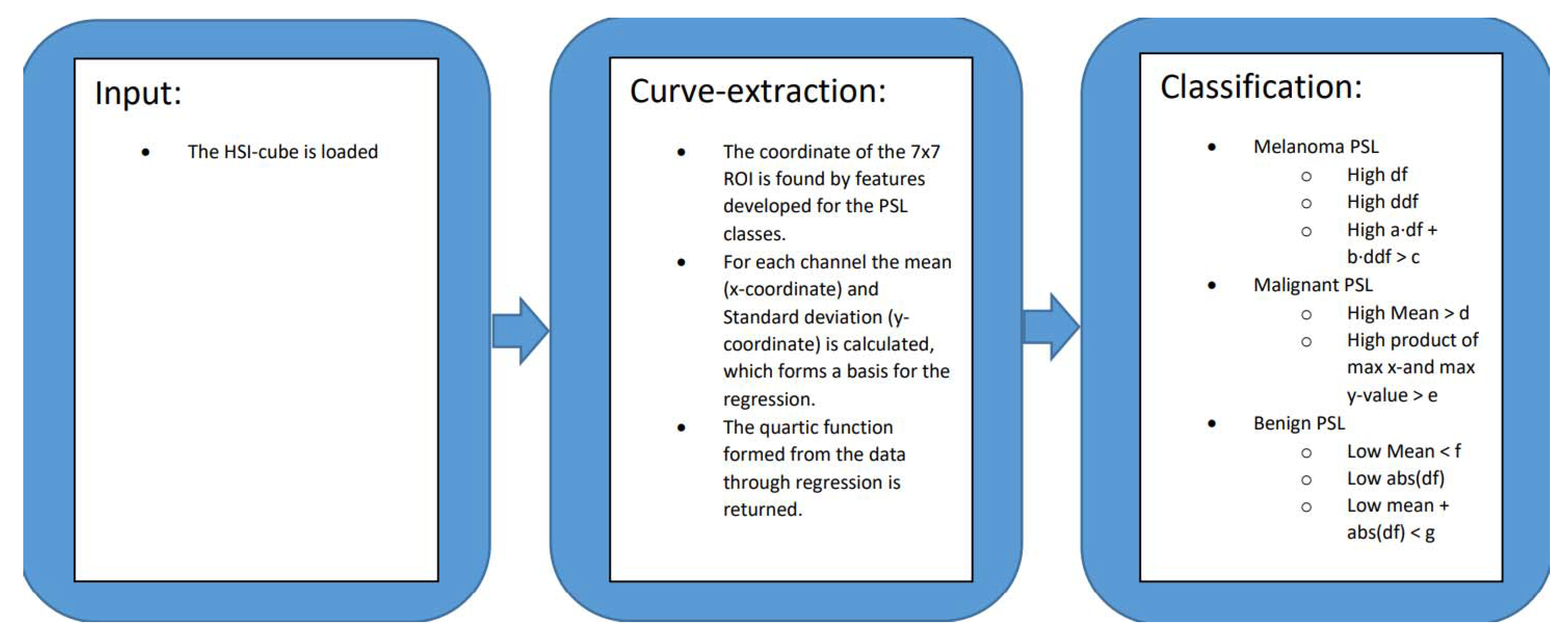
2.2. Curve-Based Classification Approach
2.3. Region of Interest Curves
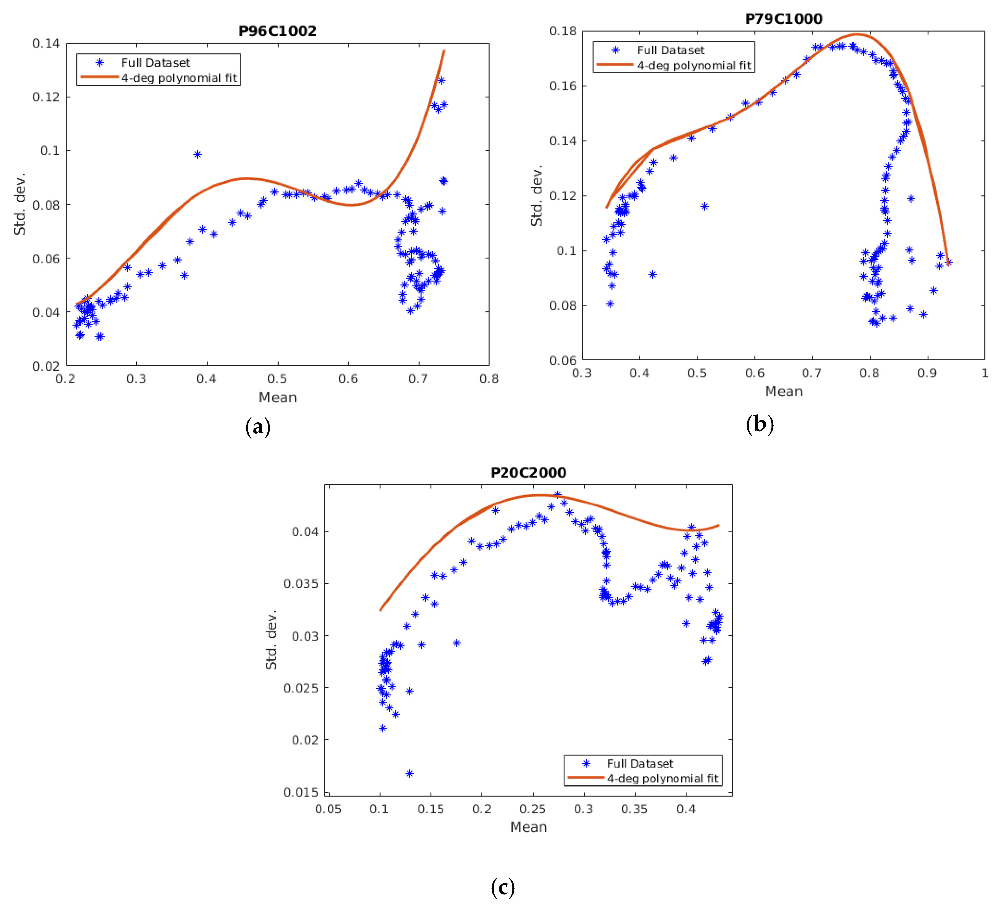
Curve-Fitting
3. Results
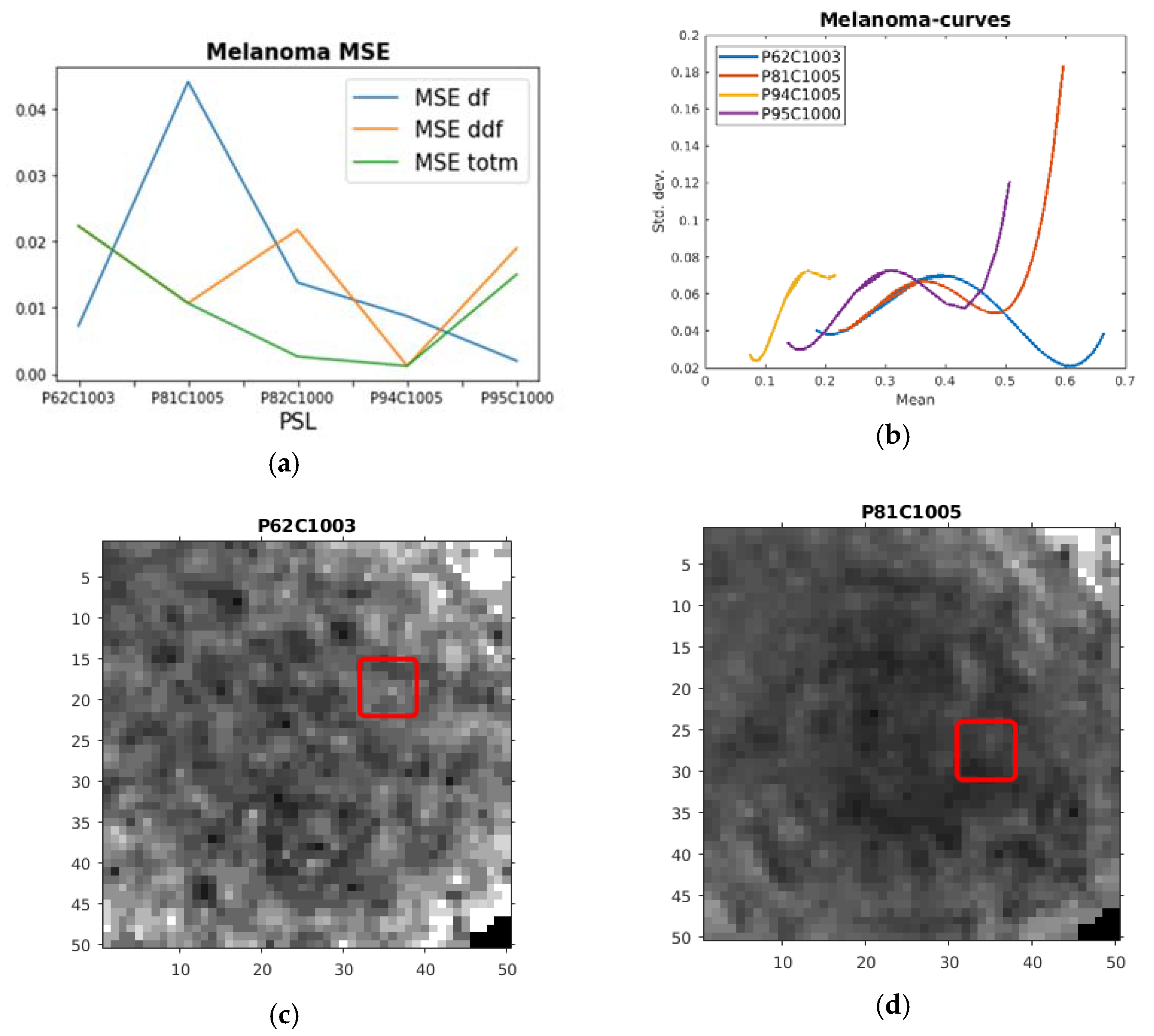
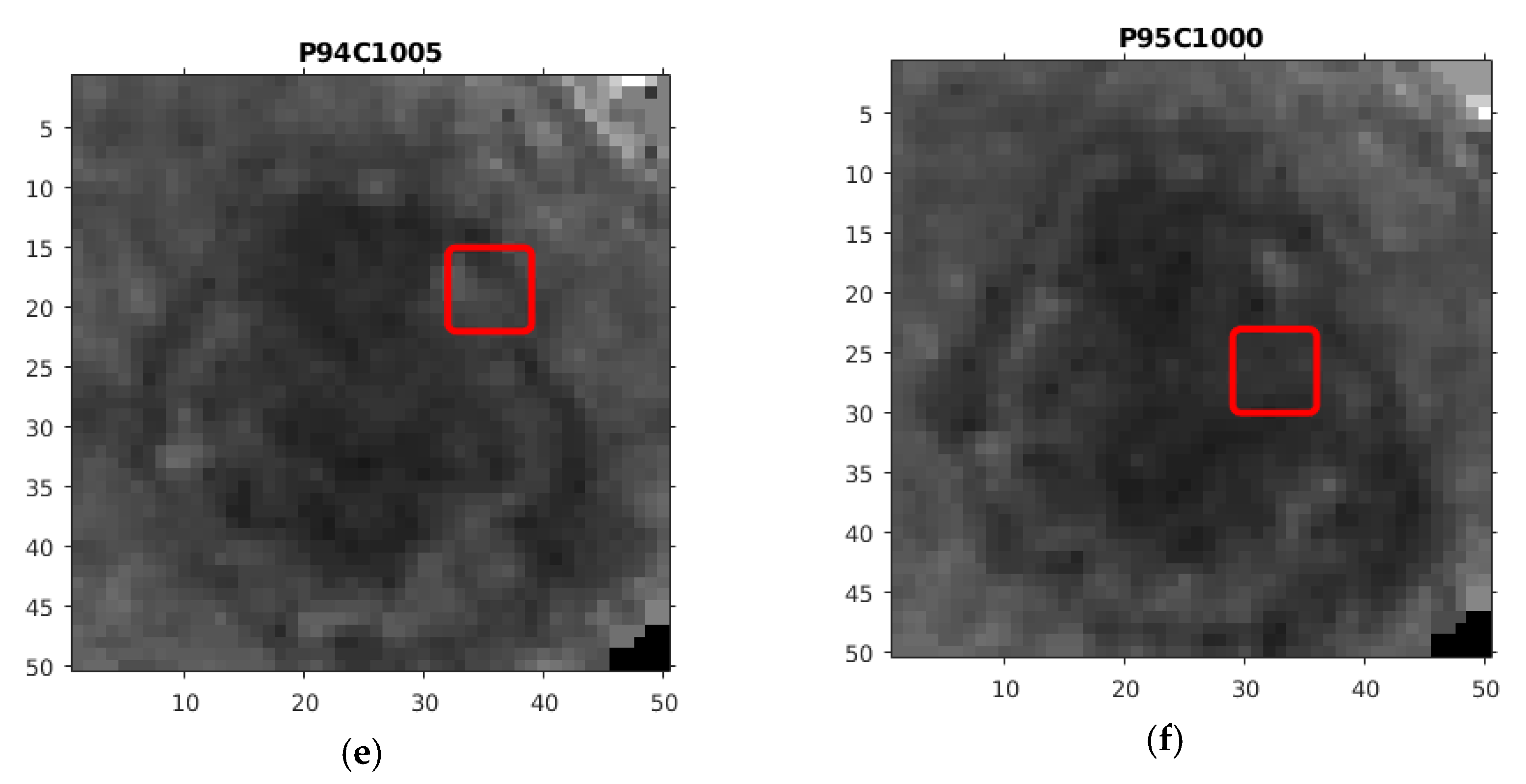
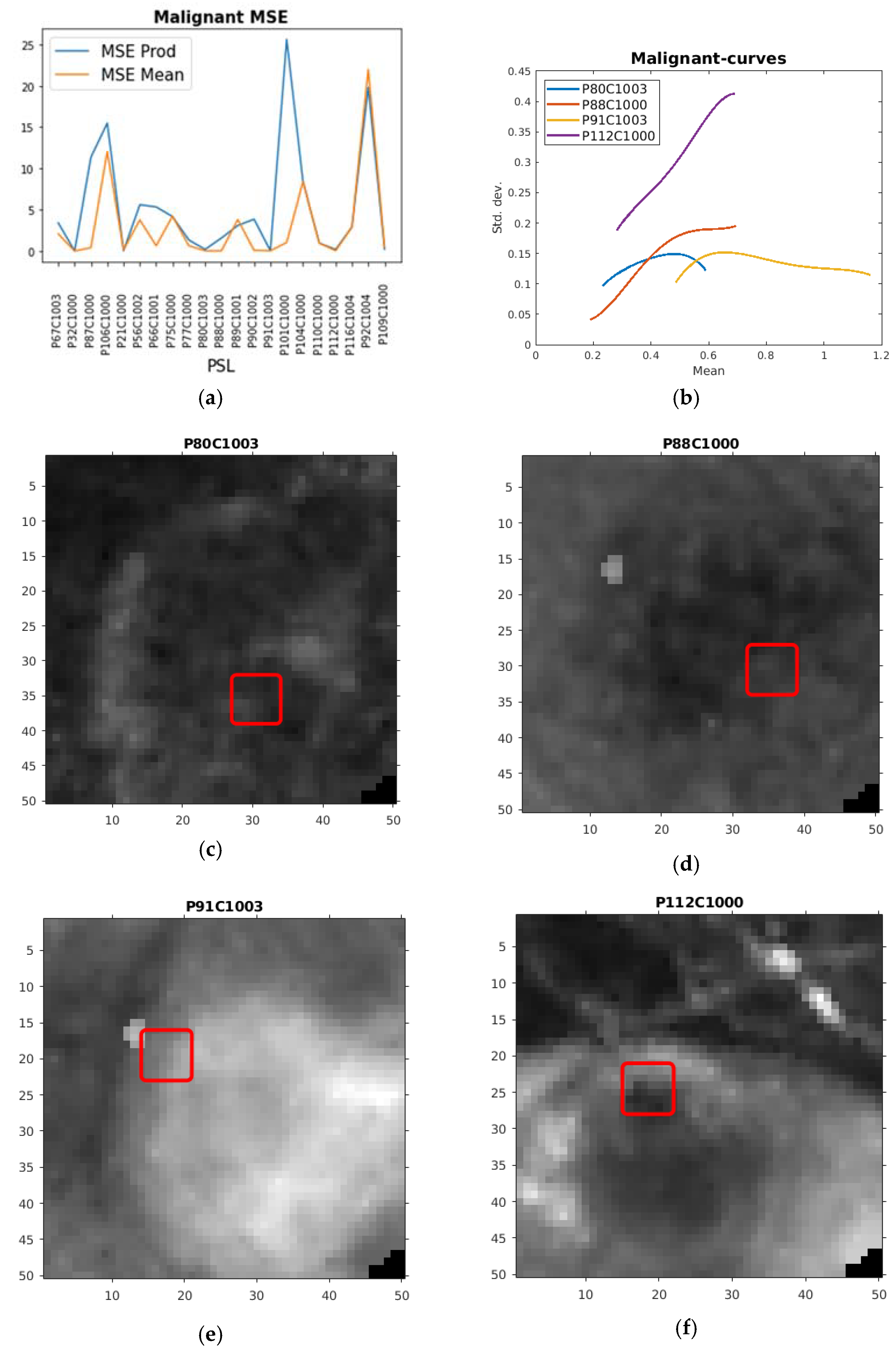
3.1. The Training Phase of the Method
Classification
3.2. Validation and Test Experiment
4. Limitations and Future Directions
5. Conclusions
Author Contributions
Funding
Institutional Review Board Statement
Informed Consent Statement
Data Availability Statement
Conflicts of Interest
References
- Hong, D.; Wu, X.; Ghamisi, P.; Chanussot, J.; Yokoya, N.; Zhu, X.X. Invariant Attribute Profiles: A Spatial-Frequency Joint Feature Extractor for Hyperspectral Image Classification. IEEE Trans. Geosci. Remote Sens. 2020, 58, 3791–3808. [Google Scholar] [CrossRef] [Green Version]
- Huang, H.; Luo, F.; Liu, L.; Yang, Y. Dimensionality reduction of hyperspectral images based on sparse discriminant manifold embedding. ISPRS J. Photogramm. Remote Sens. 2015, 106, 42–54. [Google Scholar] [CrossRef]
- Lu, G.; Fei, B. Medical hyperspectral imaging: A review. J. Biomed. Opt. 2014, 19, 010901. [Google Scholar] [CrossRef] [PubMed]
- Johansen, T.H.; Møllersen, K.; Ortega, S.; Fabelo, H.; Garcia, A.; Callico, G.M.; Godtliebsen, F. Recent advances in hyperspectral imaging for melanoma detection. Wiley Interdiscip. Rev. Comput. Stat. 2019, 12, e1465. [Google Scholar] [CrossRef]
- Bray, F.; Ferlay, J.; Soerjomataram, I.; Siegel, R.L.; Torre, L.A.; Jemal, A. Global cancer statistics 2018: GLOBOCAN estimates of incidence and mortality worldwide for 36 cancers in 185 countries. CA Cancer J. Clin. 2018, 68, 394–424. [Google Scholar] [CrossRef] [Green Version]
- LeBoit, P.E.; Burg, G.; Weedon, D.; Sarasin, A. Pathology & Genetics Skin Tumors; World Health Organization: Geneve, Switzerland, 2006. [Google Scholar]
- Tsao, H.; Olazagasti, J.M.; Cordoro, K.M.; Brewer, J.D.; Taylor, S.C.; Bordeaux, J.S.; Chren, M.-M.; Sober, A.J.; Tegeler, C.; Bhushan, R.; et al. Early detection of melanoma: Reviewing the ABCDEs American Academy of Dermatology Ad Hoc Task Force for the ABCDEs of Melanoma. J. Am. Acad. Dermatol. 2015, 72, 717–723. [Google Scholar] [CrossRef]
- Leon, R.; Martinez, B.; Fabelo, H.; Ortega, S.; Melian, V.; Castaño, I.; Carretero, G.; Almeida, P.; Garcia, A.; Quevedo, E.; et al. Non-Invasive Skin Cancer Diagnosis Using Hyperspectral Imaging for In-Situ Clinical Support. J. Clin. Med. 2020, 9, 1662. [Google Scholar] [CrossRef] [PubMed]
- Hosking, A.-M.; Coakley, B.J.; Chang, D.; Talebi-Liasi, F.; Lish, S.; Lee, S.W.; Zong, A.M.; Moore, I.; Browning, J.; Jacques, S.L.; et al. Hyperspectral imaging in automated digital dermoscopy screening for melanoma. Lasers Surg. Med. 2019, 51, 214–222. [Google Scholar] [CrossRef] [PubMed]
- Kazianka, H.; Leitner, R.; Pilz, J. Segmentation and classification of hyper-spectral skin data. In Studies in Classification, Data Analysis, and Knowledge Organization; Springer: Berlin/Heidelberg, Germany, 2008. [Google Scholar]
- Nagaoka, T.; Nakamura, A.; Kiyohara, Y.; Sota, T. Melanoma Screening System Using Hyperspectral Imager Attached to Imaging Fiberscope. In Proceedings of the Annual International Conference of the IEEE Engineering in Medicine and Biology Society, San Diego, CA, USA, 28 August–1 September 2012. [Google Scholar]
- Tomatis, S.; Carrara, M.; Bono, A.; Bartoli, C.; Lualdi, M.; Tragni, G.; Colombo, A.; Marchesini, R. Automated melanoma detection with a novel multispectral imaging system: Results of a prospective study. Phys. Med. Biol. 2005, 50, 1675–1687. [Google Scholar] [CrossRef] [PubMed]
- Moncrieff, M.D.; Cotton, S.; Claridge, E.; Hall, P. Spectrophotometric intracutaneous analysis: A new technique for imaging pigmented skin lesions. Br. J. Dermatol. 2002, 146, 448–457. [Google Scholar] [CrossRef] [PubMed]
- Fink, C.; Jaeger, C.; Jaeger, K.; Haenssle, H.A. Diagnostic performance of the MelaFind device in a real-life clinical setting. J. Dtsch. Dermatol. Ges. 2017, 15, 414–419. [Google Scholar] [CrossRef] [PubMed]
- Elbaum, M.; Kopf, A.W.; Rabinovitz, H.S.; Langley, R.G.B.; Kamino, H.; Mihm, M.C.; Sober, A.J.; Peck, G.L.; Bogdan, A.; Gutkowicz-Krusin, D.; et al. Automatic differentiation of melanoma from melanocytic nevi with multispectral digital dermoscopy: A feasibility study. J. Am. Acad. Dermatol. 2001, 44, 207–218. [Google Scholar] [CrossRef] [PubMed]
- Monheit, G.; Cognetta, A.B.; Ferris, L.; Rabinovitz, H.; Gross, K.; Martini, M.; Grichnik, J.M.; Mihm, M.; Prieto, V.G.; Googe, P.; et al. The performance of MelaFind: A prospective multicenter study. Arch. Dermatol. 2011, 147, 188–194. [Google Scholar] [CrossRef] [PubMed]
- Stamnes, J.J.; Ryzhikov, G.; Biryulina, M.; Hamre, B.; Zhao, L.; Stamnes, K. Optical detection and monitoring of pigmented skin lesions. Biomed. Opt. Express 2017, 8, 2946–2964. [Google Scholar] [CrossRef] [PubMed] [Green Version]
- Abadi, M.; Barham, P.; Chen, J.; Chen, Z.; Davis, A.; Dean, J.; Devin, M.; Ghemawat, S.; Irving, G.; Isard, M.; et al. TensorFlow: A System for Large-Scale Machine Learning. In Proceedings of the 12th USENIX Symposium on Operating Systems Design and Implementation, Savannah, GA, USA, 2–4 November 2016; pp. 265–283. [Google Scholar]
- Li, S.; Song, W.; Fang, L.; Chen, Y.; Ghamisi, P.; Benediktsson, J.A. Deep learning for hyperspectral image classification: An overview. IEEE Trans. Geosci. Remote Sens. 2019, 57, 6690–6709. [Google Scholar] [CrossRef] [Green Version]
- Fabelo, H.; Carretero, G.; Almeida, P.; Garcia, A.; Hernandez, J.A.; Godtliebsen, F.; Melian, V.; Martinez, B.; Beltran, P.; Ortega, S.; et al. Dermatologic Hyperspectral Imaging System for Skin Cancer Diagnosis Assistance. In Proceedings of the 2019 34th Conference on Design of Circuits and Integrated Systems, Bilbao, Spain, 20–22 November 2019. [Google Scholar]
- Holland, P.W.; Welsch, R.E. Robust regression using iteratively reweighted least-squares. Commun. Stat. Theory Methods 1977, 6, 813–827. [Google Scholar] [CrossRef]
- Song, E.; Grant-Kels, J.M.; Swede, H.; D’Antonio, J.L.; Lachance, A.; Dadras, S.S.; Kristjansson, A.K.; Ferenczi, K.; Makkar, H.S.; Rothe, M.J. Paired comparison of the sensitivity and specificity of multispectral digital skin lesion analysis and reflectance confocal microscopy in the detection of melanoma in vivo: A cross-sectional study. J. Am. Acad. Dermatol. 2016, 75, 1187–1192. [Google Scholar] [CrossRef] [PubMed]


| PSL | Max df | Max ddf | Max totm | MSE df | MSE ddf | MSE totm |
|---|---|---|---|---|---|---|
| P62C1003 | 0.19959 | 5.2261 | 1.2716 | 0.00729 | 0.022353 | 0.022353 |
| P81C1005 | 0.90111 | 14.465 | 5.0123 | 0.044138 | 0.010691 | 0.010691 |
| P82C1000 | 0.17383 | –0.1158 | −0.3373 | 0.01381 | 0.021781 | 0.0026241 |
| P94C1005 | 1.1388 | 45.812 | 5.0485 | 0.008742 | 0.001214 | 0.0012136 |
| P95C1000 | 0.60491 | 19.092 | 3.3212 | 0.001983 | 0.019006 | 0.015033 |
| PSL | Max Prod | Max Mean | MSE Prod | MSE Mean |
|---|---|---|---|---|
| P67C1003 | 0.20058 | 0.15051 | 3.4133 | 2.0846 |
| P32C1000 | 0.05982 | 0.054024 | 0.02244 | 0.006436 |
| P87C1000 | 0.33499 | 0.2143 | 11.323 | 0.41494 |
| P106C1000 | 0.9194 | 0.35846 | 15.474 | 11.997 |
| P21C1000 | 0.13709 | 0.11865 | 0.039819 | 0.16209 |
| P56C1002 | 0.73114 | 0.17111 | 5.6309 | 3.7864 |
| P66C1001 | 0.17669 | 0.11542 | 5.3595 | 0.64848 |
| P75C1000 | 0.36819 | 0.18003 | 4.1902 | 4.234 |
| P77C1000 | 0.31525 | 0.15402 | 1.3532 | 0.65383 |
| P80C1003 | 0.094159 | 0.13404 | 0.2015 | 0.033497 |
| P88C1000 | 0.16356 | 0.14231 | 1.5906 | 0.038208 |
| P89C1001 | 0.23628 | 0.15301 | 3.1098 | 3.8229 |
| P90C1002 | 0.33155 | 0.19675 | 3.872 | 0.087464 |
| P91C1003 | 0.1763 | 0.12843 | 0.039625 | 0.039625 |
| P101C1000 | 0.63537 | 0.24154 | 25.639 | 1.0538 |
| P104C1000 | 0.77046 | 0.20304 | 8.3724 | 8.3684 |
| P110C1000 | 0.18187 | 0.097568 | 0.96777 | 0.96777 |
| P112C1000 | 0.34958 | 0.33396 | 0.19203 | 0.045852 |
| P116C1004 | 0.26348 | 0.14593 | 2.9284 | 2.9284 |
| P92C1004 | 1.4734 | 0.28289 | 19.805 | 21.99 |
| P109C1000 | 0.38193 | 0.23467 | 0.23374 | 0.48969 |
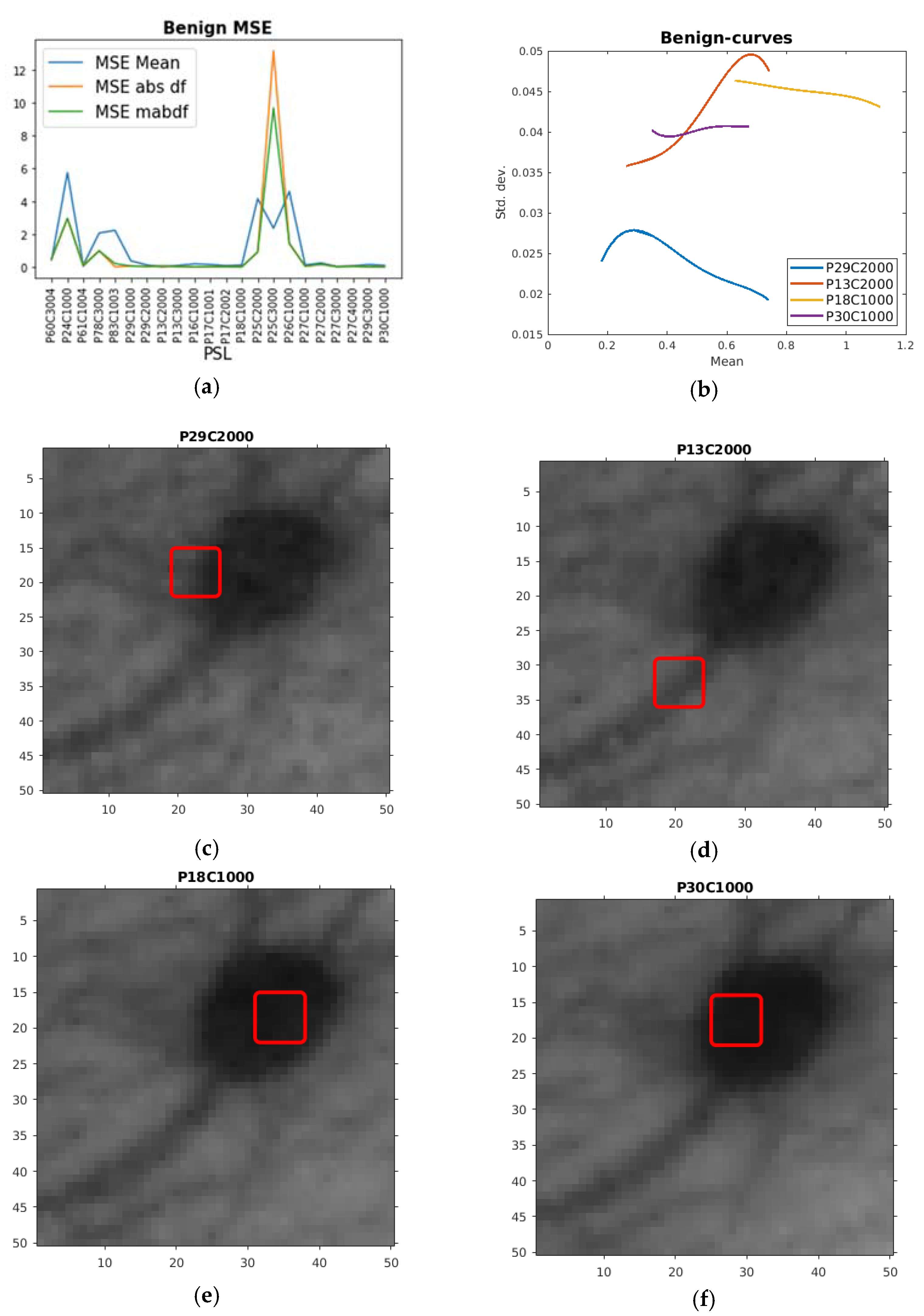
| PSL | Min Mean | Min absdf | Min mabdf | MSE Mean | MSE absdf | MSE mabdf |
|---|---|---|---|---|---|---|
| P60C3004 | 0.035875 | 0.04211 | 0.078126 | 0.43249 | 0.49182 | 0.49182 |
| P24C1000 | 0.047758 | 0.13751 | 0.20262 | 5.7292 | 2.9709 | 2.9709 |
| P61C1004 | 0.037392 | 0.019541 | 0.070525 | 0.11543 | 0.12084 | 0.049766 |
| P78C3000 | 0.054088 | 0.14207 | 0.22912 | 2.0738 | 0.98825 | 0.98825 |
| P83C1003 | 0.053259 | 0.051972 | 0.15544 | 2.2384 | 0.006806 | 0.20734 |
| P29C1000 | 0.017986 | 0.037797 | 0.067169 | 0.37593 | 0.056122 | 0.056122 |
| P29C2000 | 0.016499 | 0.028643 | 0.050963 | 0.12963 | 0.029577 | 0.029577 |
| P13C2000 | 0.018738 | 0.025028 | 0.068659 | 0.004459 | 0.018544 | 0.073912 |
| P13C3000 | 0.020795 | 0.058914 | 0.086964 | 0.097557 | 0.033792 | 0.020257 |
| P16C1000 | 0.017759 | 0.049908 | 0.073101 | 0.18981 | 0.013001 | 0.013001 |
| P17C1001 | 0.019861 | 0.021036 | 0.055137 | 0.15354 | 0.013007 | 0.028137 |
| P17C2002 | 0.023828 | 0.012184 | 0.047559 | 0.079709 | 0.020721 | 0.018856 |
| P18C1000 | 0.023887 | 0.010399 | 0.054889 | 0.11762 | 0.007339 | 0.0073387 |
| P25C2000 | 0.053336 | 0.21251 | 0.27597 | 4.1742 | 0.91204 | 0.91204 |
| P25C3000 | 0.057866 | 0.13919 | 0.22013 | 2.3664 | 13.174 | 9.6771 |
| P26C1000 | 0.050246 | 0.18733 | 0.2605 | 4.5807 | 1.4319 | 1.4319 |
| P27C1000 | 0.023408 | 0.052952 | 0.08173 | 0.12196 | 0.039168 | 0.047658 |
| P27C2000 | 0.020774 | 0.045139 | 0.069434 | 0.24855 | 0.16042 | 0.16042 |
| P27C3000 | 0.02075 | 0.058085 | 0.086034 | 0.029003 | 0.029591 | 0.016113 |
| P27C4000 | 0.019193 | 0.026195 | 0.051928 | 0.070661 | 0.037739 | 0.037739 |
| P29C3000 | 0.017297 | 0.042738 | 0.068037 | 0.14874 | 0.01073 | 0.022491 |
| P30C1000 | 0.02094 | 0.00574 | 0.045026 | 0.09903 | 0.001885 | 0.0032779 |
| PSL | Correctness |
|---|---|
| P100C1000 | tp |
| P23C1001 | fp |
| P102C1000 | tp |
| P28C1000 | tn |
| P107C1003 | tn |
| P69C1003 | tp |
| P13C1000 | tn |
| P74C1002 | tp |
| P14C1000 | tn |
| P97C1004 | tp |
| References | Patients | Images | Bands | Range (nm) | Sensitivity (%) | Specificity (%) |
|---|---|---|---|---|---|---|
| Tomatis et al. [12] | 1278 | 1391 | 15 | 483–950 | 80.4 * | 75.6 |
| Kazianka et al. [10] | - | 310 | 300 | - | 95 * | - |
| Moncrieff et al. [13] | 311 | 348 | 8 | 400–1000 | 100 *, ¥ | 5.5 |
| Fink et al. [14] | 111 | 360 | 10 | 430–950 | 100 *, ¥ | 5.5 |
| Song et al. [22] | 55 | 36 | 10 | 430–950 | 71.4 *, α | 25 |
| Monheit et al. [16] | 1257 | 1612 | 10 | 430–950 | 98.2 * | 9.5 |
| Nagaoka et al. [11] | 97 | 134 | 124 | 380–780 | 96.0 * | 87 |
| Stamnes et al. [17] | - | 157 | 10 | 365–1000 | 97 | 97 |
| Stamnes et al. [17] | - | 712 | 10 | 365–1000 | 99 | 93 |
| Hosking et al. [9] | 100 | 52 | 21 | 350–950 | 36 * | 100 * |
| Leon et al. [8] | 61 | 76 | 116 | 450–950 | 87.5/100 * | 100 |
| Proposed | 61 | 76 | 125 | 450–950 | 100 | 80/100 * |
Publisher’s Note: MDPI stays neutral with regard to jurisdictional claims in published maps and institutional affiliations. |
© 2021 by the authors. Licensee MDPI, Basel, Switzerland. This article is an open access article distributed under the terms and conditions of the Creative Commons Attribution (CC BY) license (http://creativecommons.org/licenses/by/4.0/).
Share and Cite
Uteng, S.; Quevedo, E.; M. Callico, G.; Castaño, I.; Carretero, G.; Almeida, P.; Garcia, A.; A. Hernandez, J.; Godtliebsen, F. Curve-Based Classification Approach for Hyperspectral Dermatologic Data Processing. Sensors 2021, 21, 680. https://doi.org/10.3390/s21030680
Uteng S, Quevedo E, M. Callico G, Castaño I, Carretero G, Almeida P, Garcia A, A. Hernandez J, Godtliebsen F. Curve-Based Classification Approach for Hyperspectral Dermatologic Data Processing. Sensors. 2021; 21(3):680. https://doi.org/10.3390/s21030680
Chicago/Turabian StyleUteng, Stig, Eduardo Quevedo, Gustavo M. Callico, Irene Castaño, Gregorio Carretero, Pablo Almeida, Aday Garcia, Javier A. Hernandez, and Fred Godtliebsen. 2021. "Curve-Based Classification Approach for Hyperspectral Dermatologic Data Processing" Sensors 21, no. 3: 680. https://doi.org/10.3390/s21030680