
An Overdispersed Black-Box Variational Bayesian–Kalman Filter with Inaccurate Noise Second-Order Statistics

 ,
,
Abstract
:1. Introduction
2. Materials and Methods
2.1. Kalman Filter
2.2. Introduction to Bayesian Robust Filters
2.3. Bayesian Robust Kalman Filter Based on Posterior Noise Statistics
2.3.1. KFPNS Framework
2.3.2. The Calculation Method of Posterior Noise Statistics
| Algorithm 1: KFPNS. |
| 1: input: |
| 2: output: |
| 3: Initialize |
| 4: |
| 5: |
| 6: |
| 7: |
| 8: for do |
| 9: |
| 10: |
| 11: |
| 12: |
| 13: |
| return |
| 14: end for |
| Algorithm 2: O-BBVI. |
| 1: function O-BBVI |
| 2: |
| 3: While the algorithm has not converged do |
| 4: Draw |
| 5: for to do |
| 6: Draw samples |
| 7: |
| 8: for to do |
| 9: |
| 10: |
| 11: |
| 12: |
| 13: |
| 14: end for |
| 15: |
| 16: |
| 17: end for |
| 18: for to do |
| 19: |
| 20: |
| 21: end for |
| 22: set up |
| 23: |
| 24: |
| 25: |
| return |
3. Results
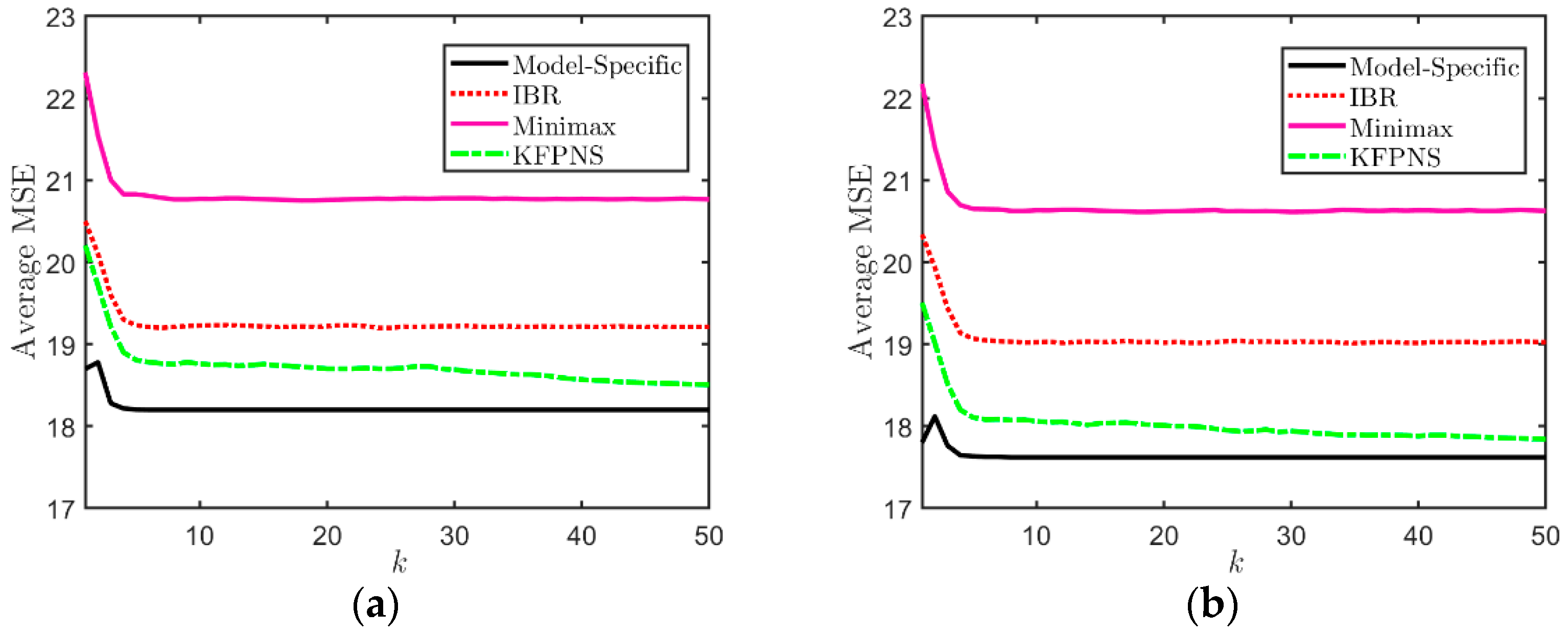
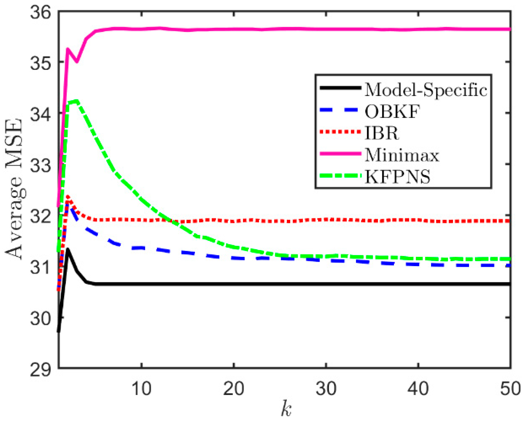
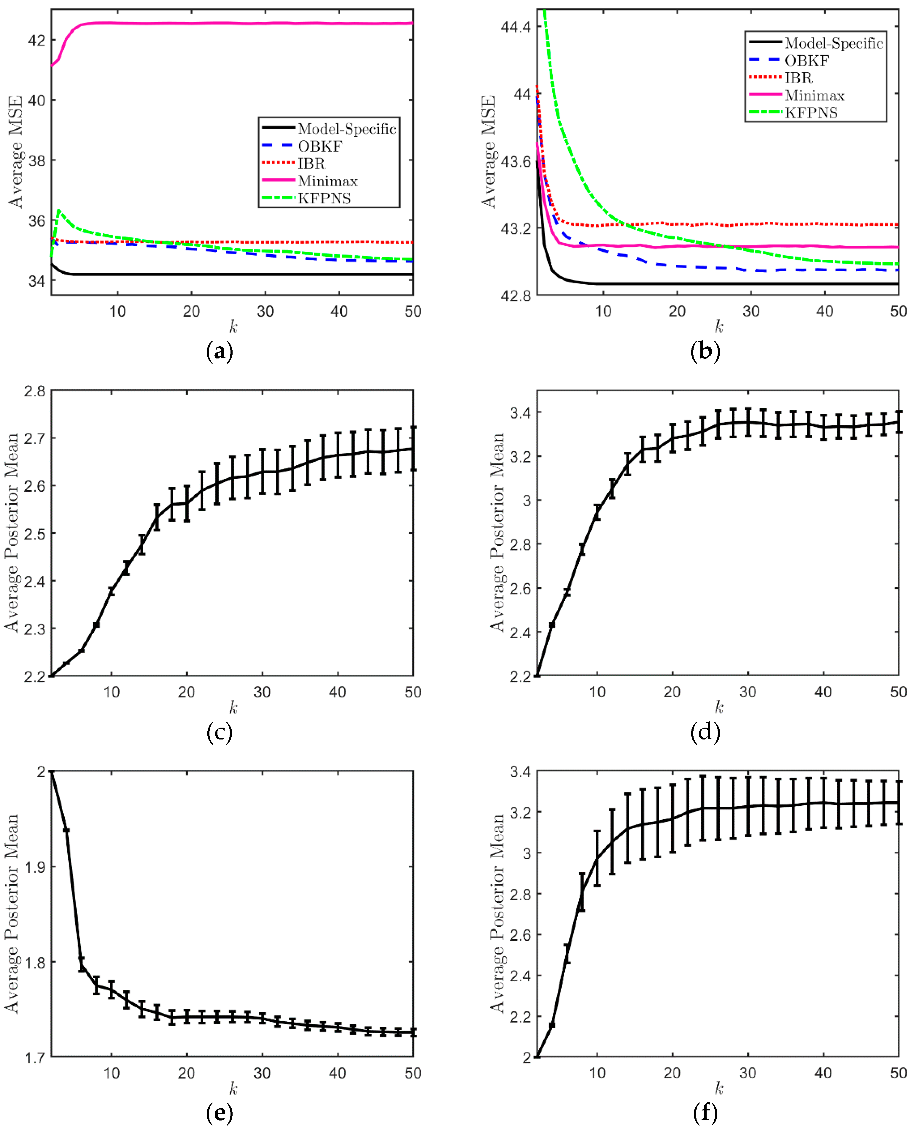
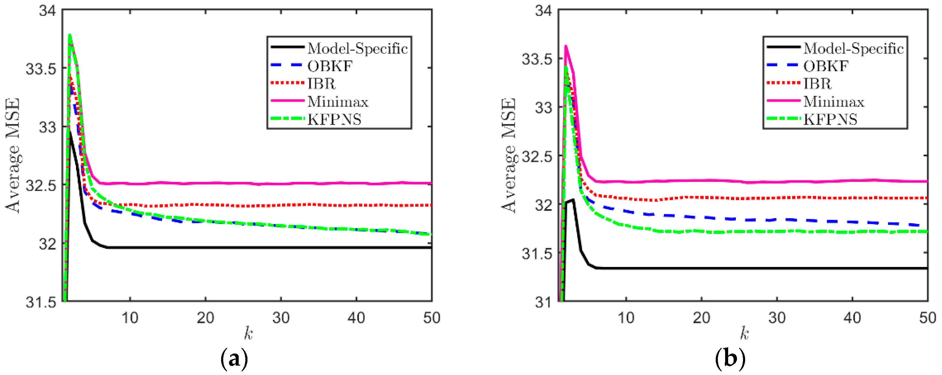
3.1. Simulation
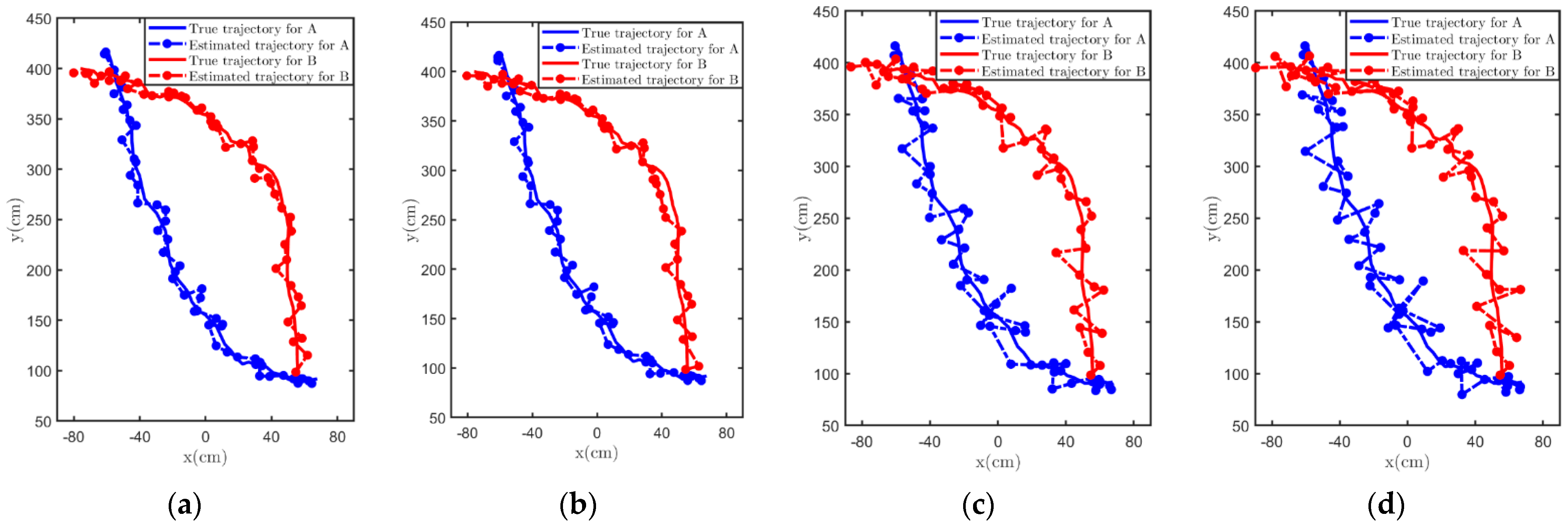
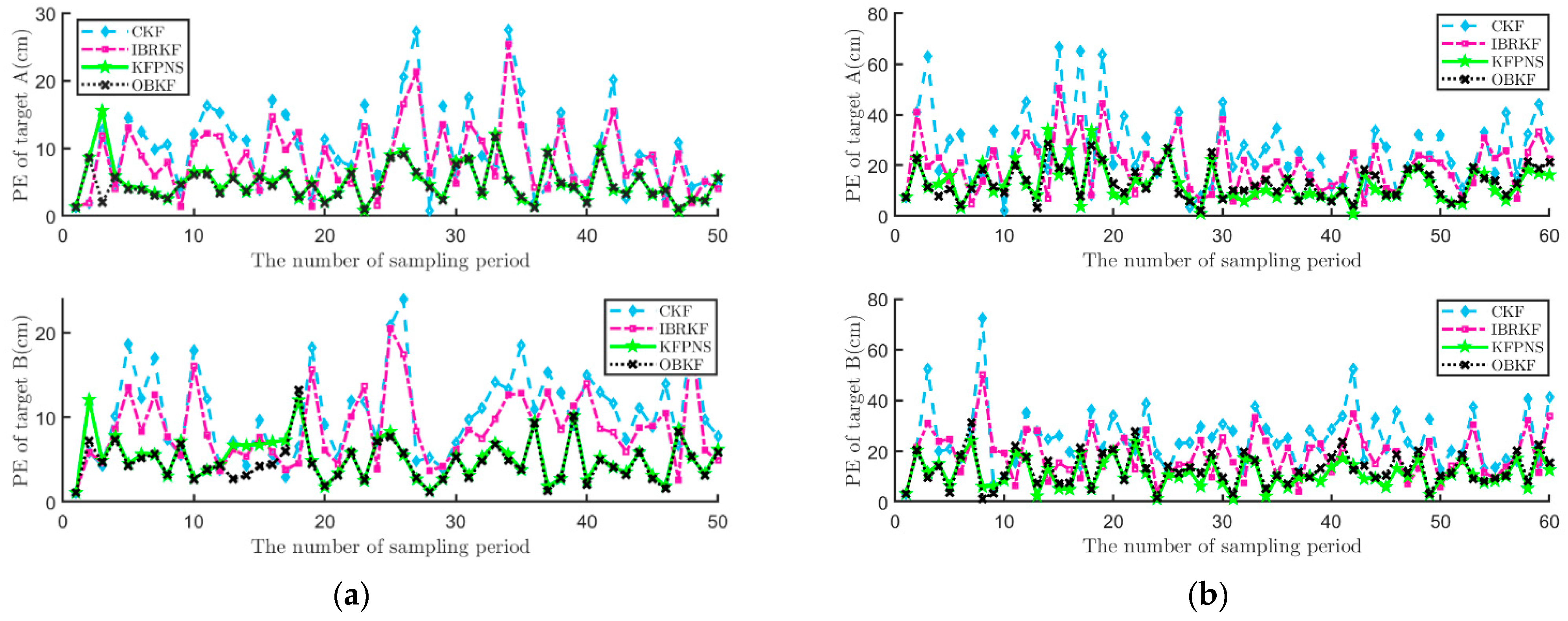
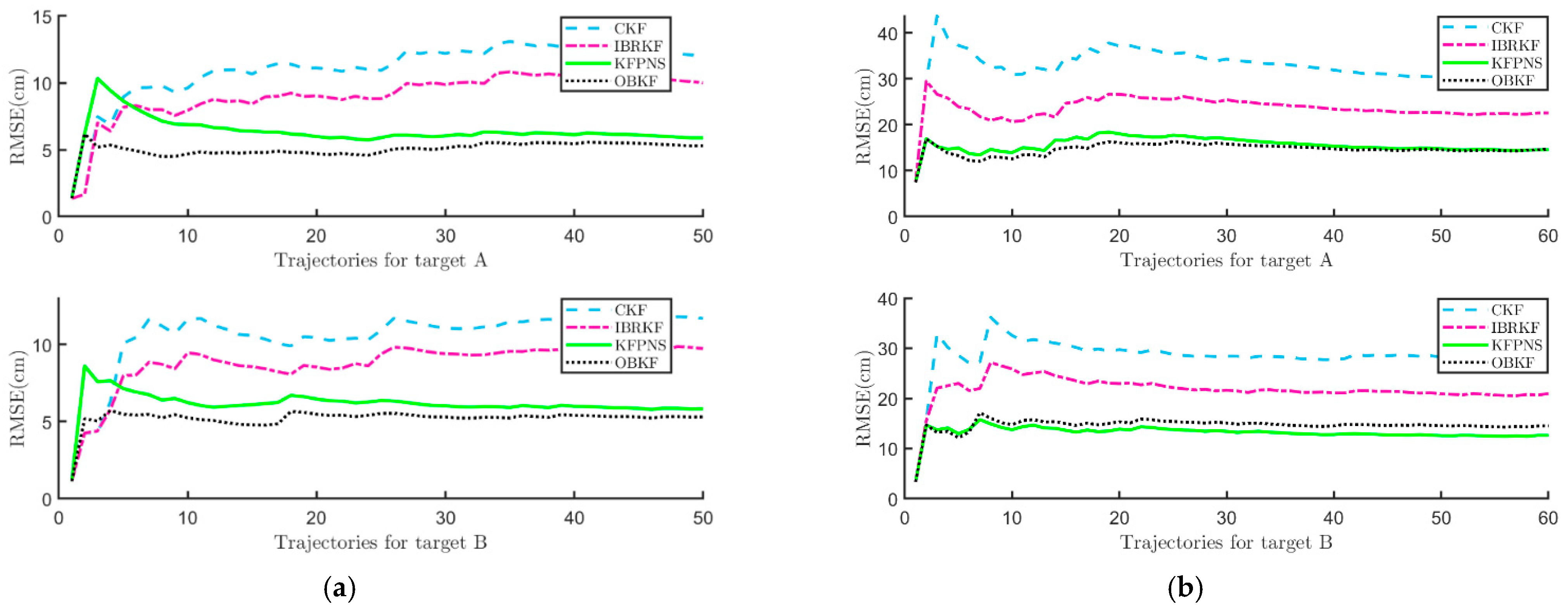
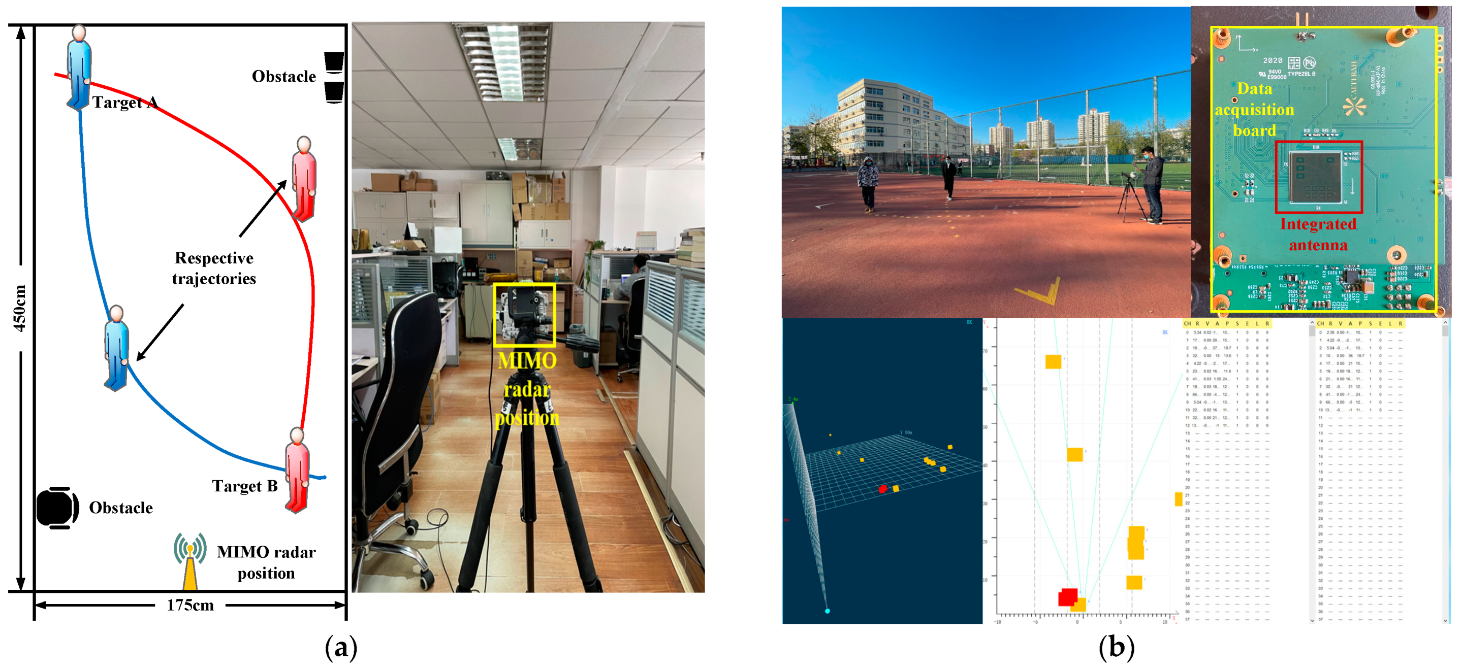
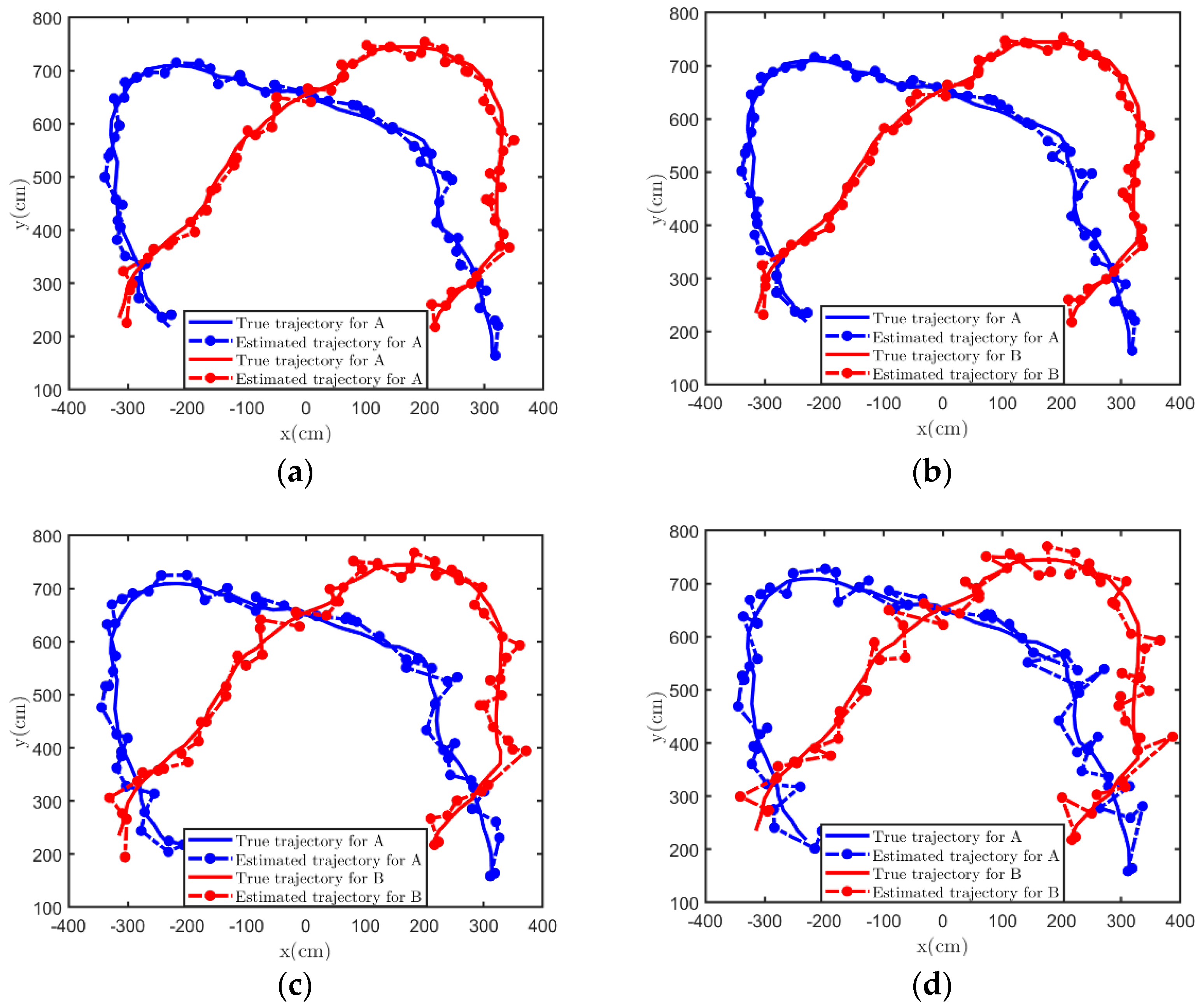
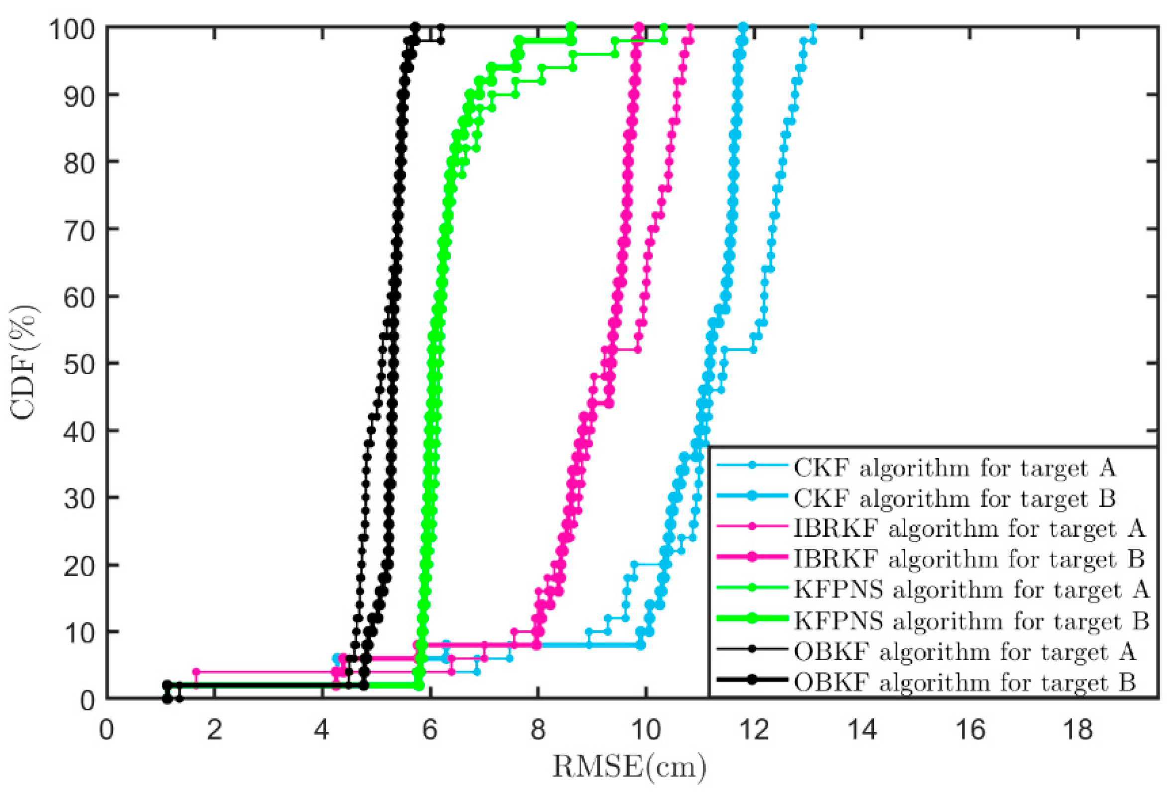
3.2. Experiment
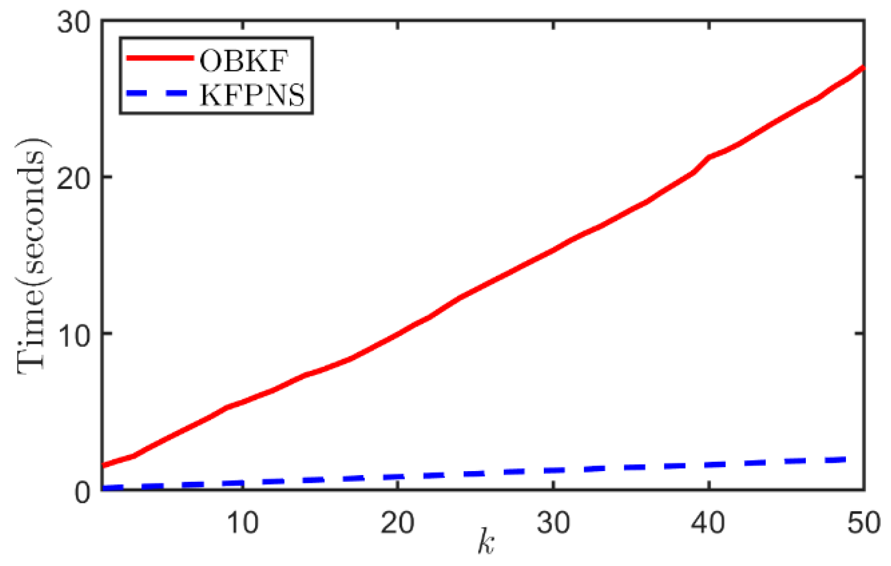
3.3. Time Cost Analysis
4. Discussion
Author Contributions
Funding
Institutional Review Board Statement
Informed Consent Statement
Data Availability Statement
Conflicts of Interest
References
- Kuznetsov, V.P. Stable detection when the signal and spectrum of normal noise are inaccurately known. Telecommun. Radio Eng. 1976, 3031, 58–64. [Google Scholar]
- Kassam, S.A.; Lim, T.L. Robust Wiener filters. J. Frankl. Inst. 1977, 304, 171–185. [Google Scholar] [CrossRef]
- Kalman, R.E. A new approach to linear filtering prediction problems. J. Basic Eng. 1960, 82, 35–45. [Google Scholar] [CrossRef] [Green Version]
- Kia, S.S.; Rounds, S.; Martinez, S. Cooperative Localization for Mobile Agents: A Recursive Decentralized Algorithm Based on Kalman-Filter Decoupling. IEEE ControlSyst. Mag. 2016, 36, 86–101. [Google Scholar]
- Bouzera, N.; Oussalah, M.; Mezhoud, N.; Khireddine, A. Fuzzy extended Kalman filter for dynamic mobile localization in urban area using wireless network. Appl. Soft Comput. 2017, 57, 452–467. [Google Scholar] [CrossRef] [Green Version]
- Safaei, A.; Mahyuddin, M.N. Adaptive Cooperative Localization Using Relative Position Estimation for Networked Systems with Minimum Number of Communication Links. IEEE Access 2019, 7, 32368–32382. [Google Scholar] [CrossRef]
- He, J.J.; Sun, C.K.; Zhang, B.S.; Wang, P. Variational Bayesian-Based Maximum Correntropy Cubature Kalman Filter with Both Adaptivity and Robustness. IEEE Sens. J. 2021, 21, 1982–1992. [Google Scholar] [CrossRef]
- Narasimhappa, M.; Mahindrakar, A.D.; Guizilini, V.C.; Terra, M.H.; Sabat, S.L. MEMS-Based IMU Drift Minimization: Sage Husa Adaptive Robust Kalman Filtering. IEEE Sens. J. 2020, 20, 250–260. [Google Scholar] [CrossRef]
- Or, B.; Bobrovsky, B.Z.; Klein, I. Kalman Filtering with Adaptive Step Size Using a Covariance-Based Criterion. IEEE Trans. Instrum. Meas. 2021, 70, 1–10. [Google Scholar] [CrossRef]
- Sarkka, S.; Nummenmaa, A. Recursive noise adaptive Kalman filtering by variational Bayesian approximations. IEEE Trans. Autom. Control 2009, 54, 596–600. [Google Scholar] [CrossRef]
- Wu, F.; Luo, H.Y.; Jia, H.W.; Zhao, F.; Xiao, Y.M.; Gao, X.L. Predicting the Noise Covariance with a Multitask Learning Model for Kalman Filter-Based GNSS/INS Integrated Navigation. IEEE Trans. Instrum. Meas. 2021, 70, 1–13. [Google Scholar] [CrossRef]
- Xu, H.; Yuan, H.D.; Duan, K.Q.; Xie, W.C.; Wang, Y.L. An Adaptive Gaussian Sum Kalman Filter Based on a Partial Variational Bayesian Method. IEEE Trans. Autom. Control 2020, 65, 4793–4799. [Google Scholar] [CrossRef]
- Yasini, S.; Pelckmans, K. Worst-Case Prediction Performance Analysis of the Kalman Filter. IEEE Trans. Autom. Control 2018, 63, 1768–1775. [Google Scholar] [CrossRef] [Green Version]
- Zorzi, M. Robust Kalman Filtering Under Model Perturbations. IEEE Trans. Autom. Control 2017, 62, 2902–2907. [Google Scholar] [CrossRef] [Green Version]
- Morris, J.M. The Kalman filter: A robust estimator for some classes of linear quadratic problems. IEEE Trans. Inf. Theory 1976, 22, 526–534. [Google Scholar] [CrossRef]
- Shmaliy, Y.S. An iterative Kalman-like algorithm ignoring noise and initial conditions. IEEE Trans. Signal Process. 2011, 59, 2465–2473. [Google Scholar] [CrossRef]
- Shmaliy, Y.S.; Lehmann, F.; Zhao, S.; Ahn, C.K. Comparing Robustness of the Kalman, H∞, and UFIR Filters. IEEE Trans. Signal Process. 2018, 66, 3447–3458. [Google Scholar] [CrossRef]
- Shmaliy, Y.S. Linear optimal FIR estimation of discrete time-invariant state-space models. IEEE Trans. Signal Process. 2010, 58, 3086–3096. [Google Scholar] [CrossRef]
- Zhao, S.Y.; Shmaliy, Y.S.; Liu, F. Fast Kalman-Like Optimal Unbiased FIR Filtering with Applications. IEEE Trans. Signal Process. 2016, 64, 2284–2297. [Google Scholar] [CrossRef]
- Dehghannasiri, R.; Esfahani, M.S.; Dougherty, E.R. Intrinsically Bayesian robust Kalman filter: An innovation process approach. IEEE Trans. Signal Process. 2017, 65, 2531–2546. [Google Scholar] [CrossRef]
- Dehghannasiri, R.; Esfahani, M.S.; Qian, X.N.; Dougherty, E.R. Optimal Bayesian Kalman Filtering with Prior Update. IEEE Trans. Signal Process. 2018, 66, 1982–1996. [Google Scholar] [CrossRef]
- Lei, X.; Li, J. An Adaptive Altitude Information Fusion Method for Autonomous Landing Processes of Small Unmanned Aerial Rotorcraft. Sensors 2012, 12, 13212–13224. [Google Scholar] [CrossRef] [Green Version]
- Xu, G.; Huang, Y.; Gao, Z.; Zhang, Y. A Computationally Efficient Variational Adaptive Kalman Filter for Transfer Alignment. IEEE Sens. J. 2020, 20, 13682–13693. [Google Scholar] [CrossRef]
- Shan, C.; Zhou, W.; Yang, Y.; Jiang, Z. Multi-Fading Factor and Updated Monitoring Strategy Adaptive Kalman Filter-Based Variational Bayesian. Sensors 2021, 21, 198. [Google Scholar] [CrossRef] [PubMed]
- Huang, Y.; Zhang, Y.; Wu, Z.; Li, N.; Chambers, J. A Novel Adaptive Kalman Filter with Inaccurate Process and Measurement Noise Covariance Matrices. IEEE Trans. Autom. Control 2018, 63, 594–601. [Google Scholar] [CrossRef] [Green Version]
- Zhang, Y.; Jia, G.; Li, N.; Bai, M. A Novel Adaptive Kalman Filter with Colored Measurement Noise. IEEE Access 2018, 6, 74569–74578. [Google Scholar] [CrossRef]
- Kailath, T. An innovations approach to least-squares estimation—Part I: Linear filtering in additive white noise. IEEE Trans. Autom. Control 1968, AC-13, 646–655. [Google Scholar] [CrossRef]
- Zadeh, L.A.; Ragazzini, J.R. An extension of Wiener’s theory of prediction. J. Appl. Phys. 1950, 21, 645–655. [Google Scholar] [CrossRef]
- Bode, H.W.; Shannon, C.E. A simplified derivation of linear least square smoothing and prediction theory. Proc. IRE 1950, 38, 417–425. [Google Scholar] [CrossRef]
- Poor, H.V. On robust Wiener filtering. IEEE Trans. Autom. Control 1980, 25, 531–536. [Google Scholar] [CrossRef]
- Vastola, K.S.; Poor, H.V. Robust Wiener-Kolmogorov theory. IEEE Trans. Inf. Theory 1984, 30, 316–327. [Google Scholar] [CrossRef]
- Poor, H.V. Robust matched filters. IEEE Trans. Inf. Theory 1983, 29, 677–687. [Google Scholar] [CrossRef]
- Ruiz, F.J.; Titsias, M.; Blei, D.M. Overdispersed Black-Box Variational Inference. In Proceedings of the Thirty-Second Conference on Uncertainty in Artificial Intelligence, Jersey City, NJ, USA, 25–29 June 2016; pp. 647–656. [Google Scholar]
- Duchi, J.; Hazan, E.; Singer, Y. Adaptive subgradient methods for online learning and stochastic optimization. J. Mach. Learn. Res. 2011, 12, 2121–2159. [Google Scholar]


| Classical Kalman Filter | KFPNS |
|---|---|
| Radar Model | Radar System | The Start Frequency | Range Resolution | Frame Periodicity | Scan Range |
|---|---|---|---|---|---|
| RDP-77S244-ABM-AIP | FMCW | 77 GHz | 0.045 m | 200 ms | FOV 120° |
| Algorithm | MMSE | |||
|---|---|---|---|---|
| Indoor Scene | Outdoor Scene | |||
| Target A | Target B | Target A | Target B | |
| KFPNS | 6.3679 cm | 6.1552 cm | 15.5520 cm | 13.1918 cm |
| IBRKF | 9.0658 cm | 8.7459 cm | 23.5724 cm | 21.7488 cm |
| CKF | 11.0092 cm | 10.5480 cm | 32.6647 cm | 28.4253 cm |
| OBKF | 5.0358 cm | 5.2118 cm | 14.6269 cm | 14.6148 cm |
Publisher’s Note: MDPI stays neutral with regard to jurisdictional claims in published maps and institutional affiliations. |
© 2021 by the authors. Licensee MDPI, Basel, Switzerland. This article is an open access article distributed under the terms and conditions of the Creative Commons Attribution (CC BY) license (https://creativecommons.org/licenses/by/4.0/).
Share and Cite
Cao, L.; Zhang, C.; Zhao, Z.; Wang, D.; Du, K.; Fu, C.; Gu, J. An Overdispersed Black-Box Variational Bayesian–Kalman Filter with Inaccurate Noise Second-Order Statistics. Sensors 2021, 21, 7673. https://doi.org/10.3390/s21227673
Cao L, Zhang C, Zhao Z, Wang D, Du K, Fu C, Gu J. An Overdispersed Black-Box Variational Bayesian–Kalman Filter with Inaccurate Noise Second-Order Statistics. Sensors. 2021; 21(22):7673. https://doi.org/10.3390/s21227673
Chicago/Turabian StyleCao, Lin, Chuyuan Zhang, Zongmin Zhao, Dongfeng Wang, Kangning Du, Chong Fu, and Jianfeng Gu. 2021. "An Overdispersed Black-Box Variational Bayesian–Kalman Filter with Inaccurate Noise Second-Order Statistics" Sensors 21, no. 22: 7673. https://doi.org/10.3390/s21227673
APA StyleCao, L., Zhang, C., Zhao, Z., Wang, D., Du, K., Fu, C., & Gu, J. (2021). An Overdispersed Black-Box Variational Bayesian–Kalman Filter with Inaccurate Noise Second-Order Statistics. Sensors, 21(22), 7673. https://doi.org/10.3390/s21227673