
A Novel Occupancy Mapping Framework for Risk-Aware Path Planning in Unstructured Environments

 , and
, and 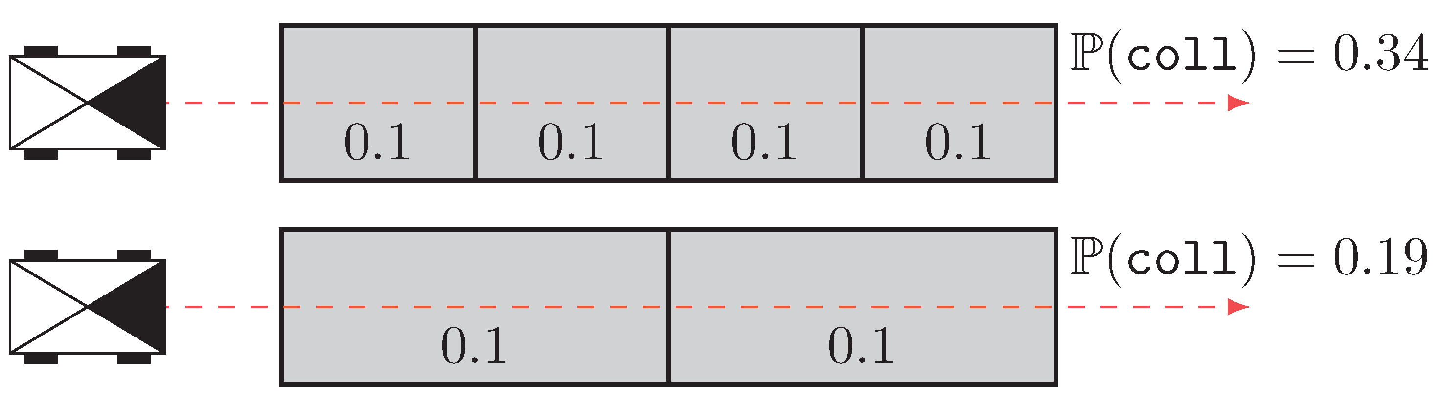
Abstract
:1. Introduction
- A novel type of map called the Lambda Field, which is specially designed to allow generic risk assessments and is better fitted for unstructured environments;
- A mathematical formulation of risk assessment over a path with an application to path planning in tall grass;
- A theoretical and experimental evaluation of the Bayesian occupancy grid, showing that such a framework can over-converge in the case of unstructured and sparse obstacles.
2. Related Work
3. Theoretical Framework
3.1. Computation of the Field
3.2. Confidence Intervals
3.3. Generic Framework for Risk Assessment
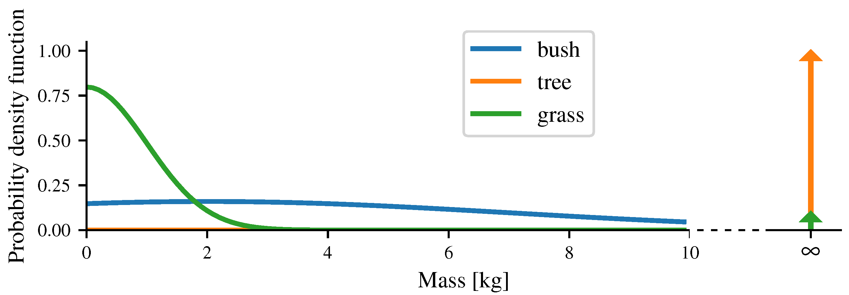
3.4. Taking into Account the Mass of the Obstacles
3.5. Comparison and Improvement of the Reachability Metric
4. Validation
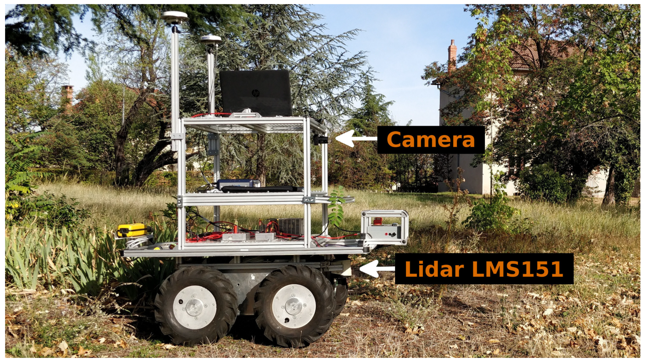
4.1. Setup
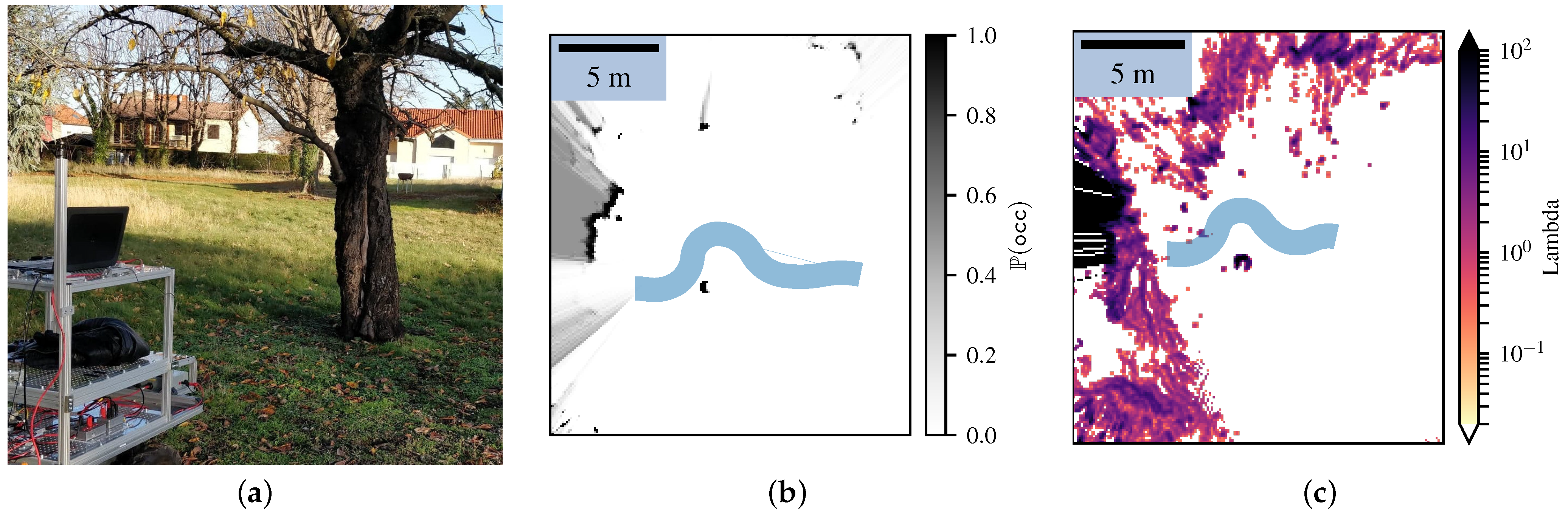
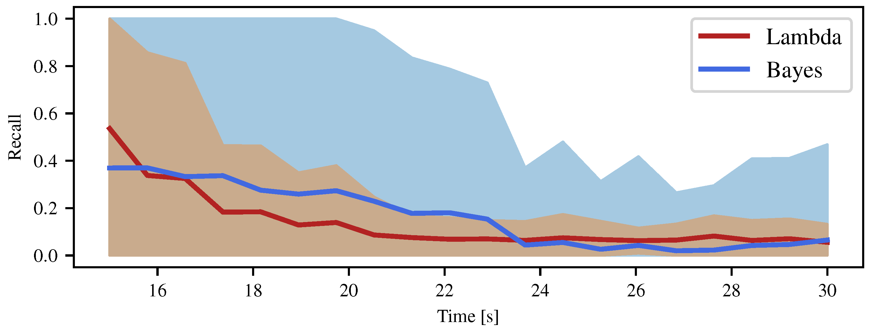
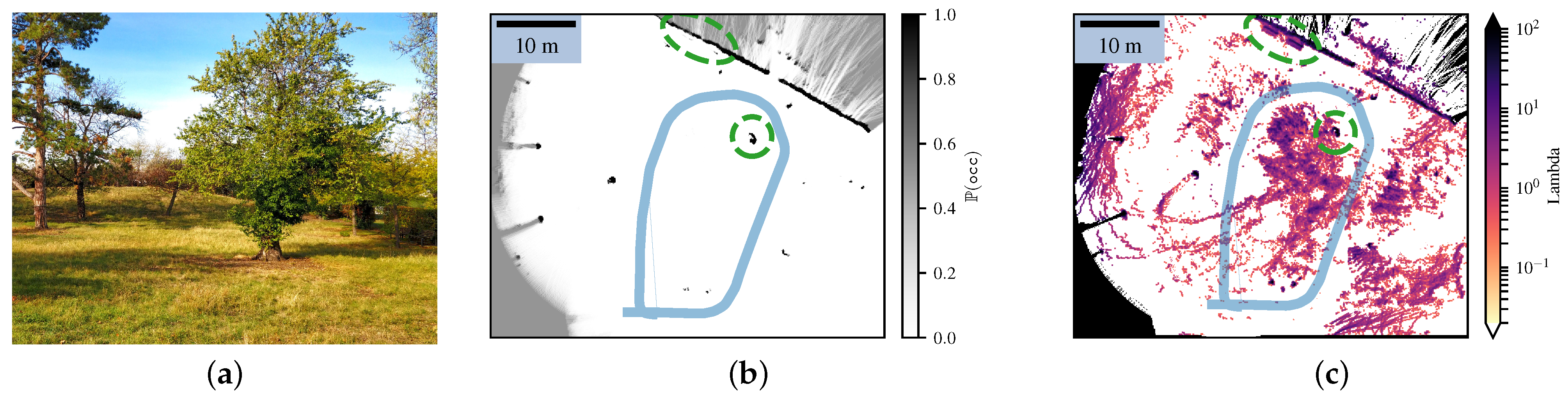
4.2. Comparison with the Bayesian Occupancy Grid
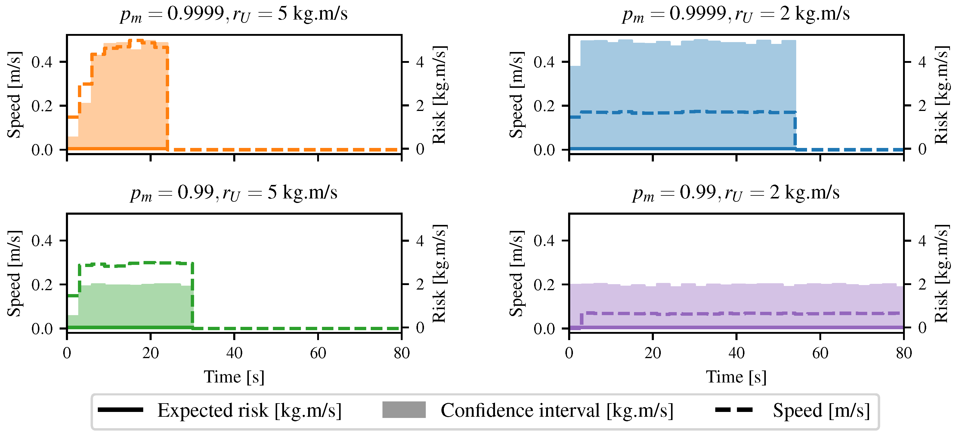
4.3. Basic Path Planning
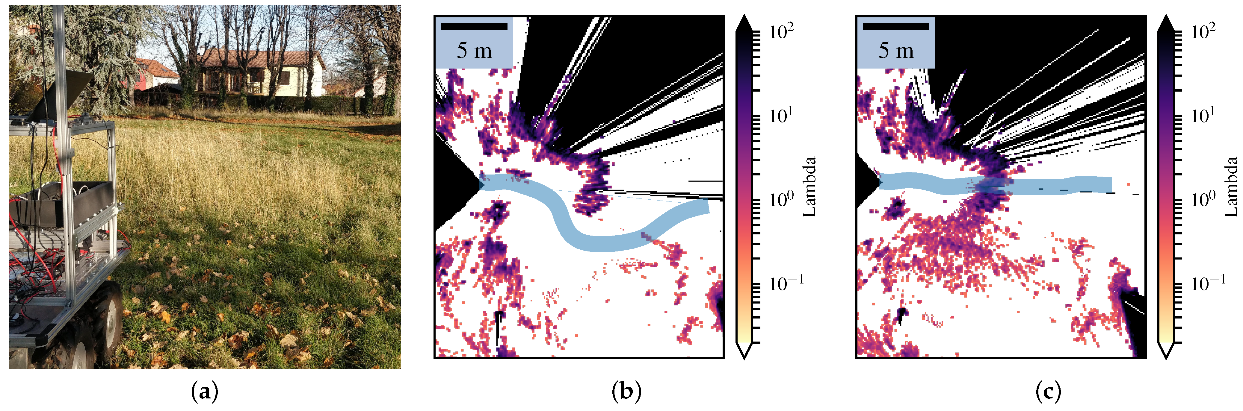
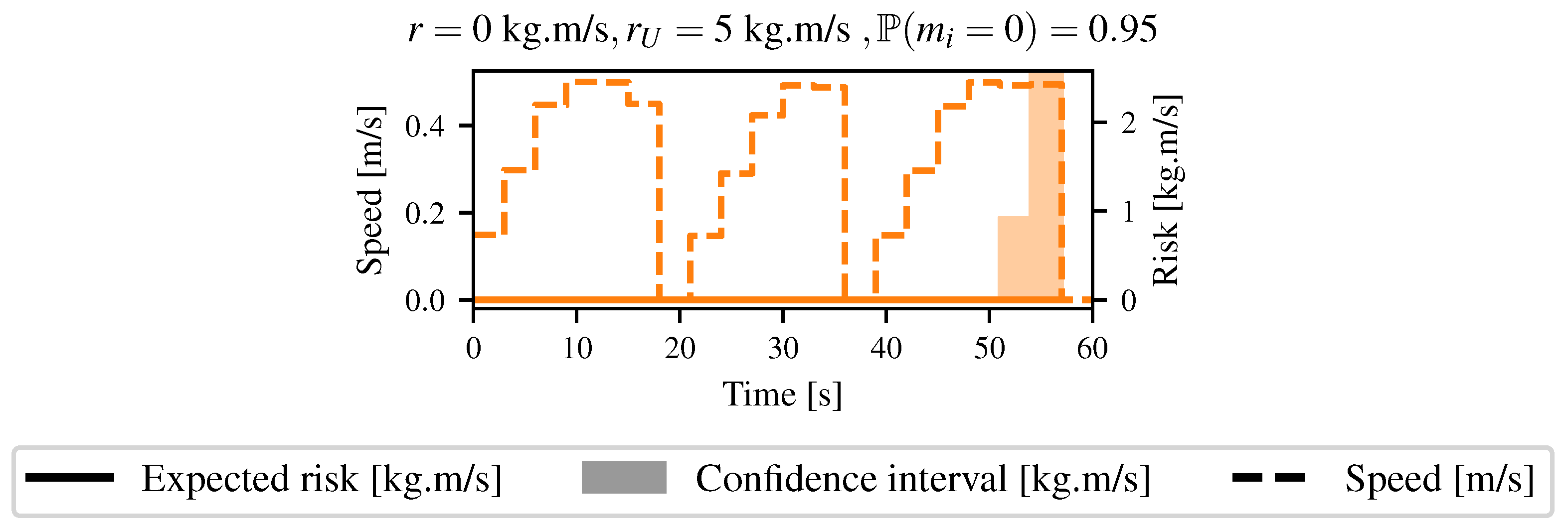
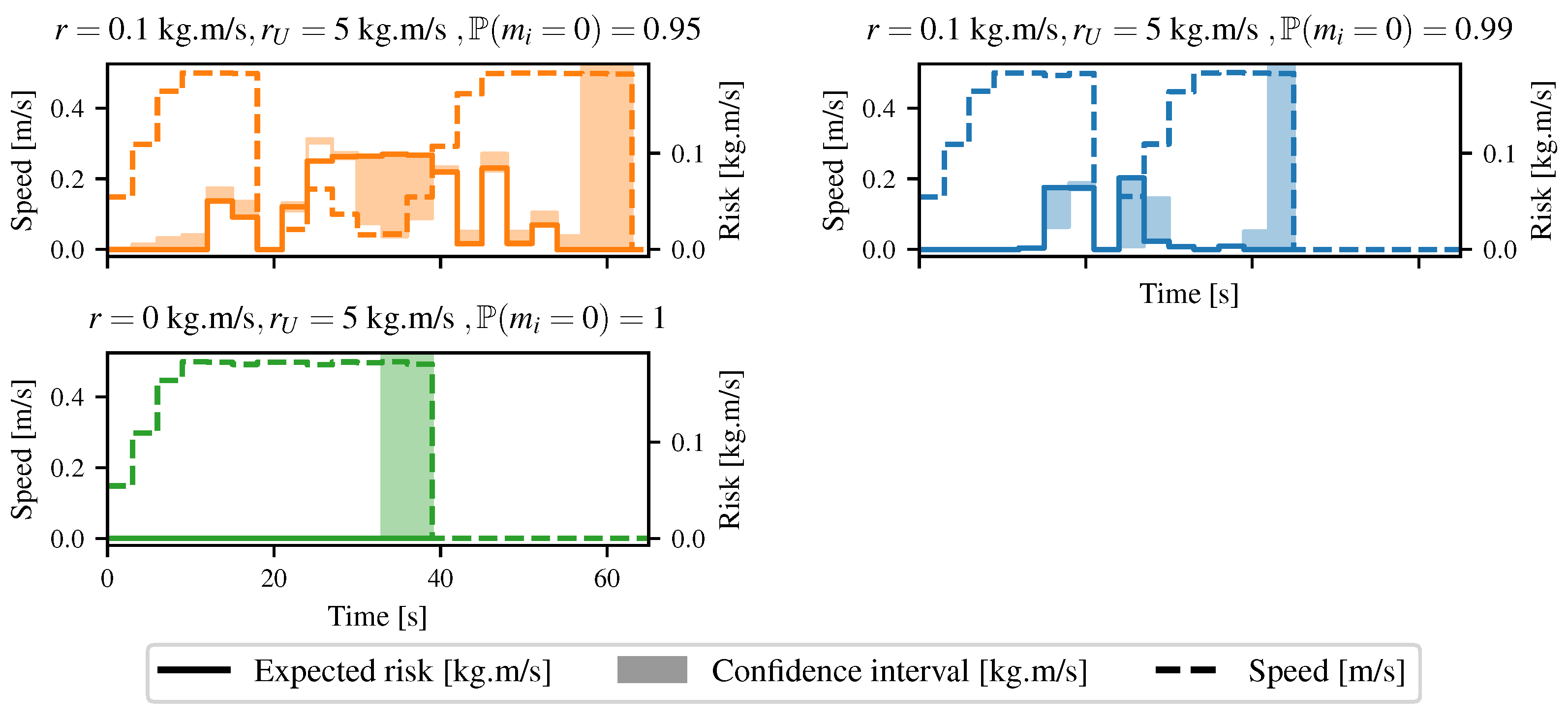
4.4. Going through Tall Grass
5. Discussion
6. Conclusions
Author Contributions
Funding
Acknowledgments
Conflicts of Interest
Appendix A. Heterogeneous Error Regions
Appendix B. Proof of Equation (26)
Appendix C. Probabilistic Error Region
References
- Fulgenzi, C.; Spalanzani, A.; Laugier, C. Dynamic obstacle avoidance in uncertain environment combining PVOs and occupancy grid. In Proceedings of the IEEE International Conference on Robotics and Automation, Roma, Italy, 10–14 April 2007; pp. 1610–1616. [Google Scholar]
- Elfes, A. Using occupancy grids for mobile robot perception and navigation. Computer 1989, 6, 46–57. [Google Scholar] [CrossRef]
- Heiden, E.; Hausman, K.; Sukhatme, G.S. Planning High-speed Safe Trajectories in Confidence-rich Maps. In Proceedings of the IEEE/RSJ International Conference on Intelligent Robots and Systems, Vancouver, BC, Canada, 24–28 September 2017; pp. 2880–2886. [Google Scholar]
- Kraetzschmar, G.K.; Gassull, G.P.; Uhl, K. Probabilistic quadtrees for variable-resolution mapping of large environments. In Proceedings of the 5th IFAC/EURON Symposium on Intelligent Autonomous Vehicles, Lisbon, Portugal, 5–7 July 2004. [Google Scholar]
- Laconte, J.; Debain, C.; Chapuis, R.; Pomerleau, F.; Aufrère, R. Lambda-Field: A Continuous Counterpart of the Bayesian Occupancy Grid for Risk Assessment. In Proceedings of the IEEE/RSJ International Conference on Intelligent Robots and Systems, Macau, China, 3–8 November 2019; pp. 167–172. [Google Scholar]
- Coué, C.; Pradalier, C.; Laugier, C.; Fraichard, T.; Bessière, P. Bayesian occupancy filtering for multitarget tracking: An automotive application. Int. J. Robot. Res. 2006, 25, 19–30. [Google Scholar] [CrossRef] [Green Version]
- Saval-Calvo, M.; Medina-Valdés, L.; Castillo-Secilla, J.M.; Cuenca-Asensi, S.; Martínez-Álvarez, A.; Villagrá, J. A review of the bayesian occupancy filter. Sensors 2017, 17, 344. [Google Scholar] [CrossRef]
- O’Callaghan, S.T.; Ramos, F.T. Gaussian process occupancy maps. Int. J. Robot. Res. 2012, 31, 42–62. [Google Scholar] [CrossRef]
- Kim, S.; Kim, J. Continuous occupancy maps using overlapping local Gaussian processes. In Proceedings of the IEEE International Conference on Intelligent Robots and Systems, Tokyo, Japan, 3–7 November 2013; pp. 4709–4714. [Google Scholar]
- Ramos, F.; Ott, L. Hilbert maps: Scalable continuous occupancy mapping with stochastic gradient descent. Int. J. Robot. Res. 2016, 35, 1717–1730. [Google Scholar] [CrossRef]
- Senanayake, R.; Ramos, F. Bayesian Hilbert Maps for Continuous Occupancy Mapping in Dynamic Environments. In Proceedings of the Conference on Robot Learning, Mountain View, CA, USA, 13–15 November 2017; pp. 458–471. [Google Scholar]
- Guizilini, V.; Senanayake, R.; Ramos, F. Dynamic hilbert maps: Real-time occupancy predictions in changing environments. In Proceedings of the IEEE International Conference on Robotics and Automation, Montreal, QC, Canada, 20–24 May 2019; pp. 4091–4097. [Google Scholar]
- Agha-mohammadi, A.A.; Heiden, E.; Hausman, K.; Sukhatme, G. Confidence-rich grid mapping. Int. J. Robot. Res. 2019, 38, 1352–1374. [Google Scholar] [CrossRef]
- Fraichard, T. A Short Paper About Motion Safety. In Proceedings of the IEEE International Conference on Robotics and Automation, Roma, Italy, 10–14 April 2007; pp. 1140–1145. [Google Scholar]
- Lee, D.N. A theory of visual control of braking based on information about time-to-collision. Perception 1976, 5, 437–459. [Google Scholar] [CrossRef] [PubMed]
- Laugier, C.; Paromtchik, I.E.; Perrollaz, M.; Yong, M.; Yoder, J.D.; Tay, C.; Mekhnacha, K.; Nègre, A. Probabilistic analysis of dynamic scenes and collision risks assessment to improve driving safety. IEEE Intell. Transp. Syst. Mag. 2011, 3, 4–19. [Google Scholar] [CrossRef] [Green Version]
- Vaillant, M.; Davatzikos, C.; Taylor, R.H.; Bryan, R.N. A Path-Planning Algorithm for Image-Guided Neurosurgery. In Proceedings of the CVRMed-MRCAS’97, Grenoble, France, 19–22 March 1997; pp. 467–476. [Google Scholar]
- Caborni, C.; Ko, S.Y.; De Momi, E.; Ferrigno, G.; Y Baena, F.R. Risk-based path planning for a steerable flexible probe for neurosurgical intervention. In Proceedings of the IEEE RAS and EMBS International Conference on Biomedical Robotics and Biomechatronics, Rome, Italy, 24–27 June 2012; pp. 866–871. [Google Scholar]
- Majumdar, A.; Pavone, M. How Should a Robot Assess Risk? Towards an Axiomatic Theory of Risk in Robotics. In Robotics Research; Springer International Publishing: Cham, Switzerland, 2020; pp. 75–84. [Google Scholar]
- Tsiotras, P.; Bakolas, E. A hierarchical on-line path planning scheme using wavelets. In Proceedings of the 2007 European Control Conference, ECC 2007, Kos, Greece, 2–5 July 2007; pp. 2806–2812. [Google Scholar]
- De Filippis, L.; Guglieri, G.; Quagliotti, F. A minimum risk approach for path planning of UAVs. J. Intell. Robot. Syst. Theory Appl. 2011, 61, 203–219. [Google Scholar] [CrossRef]
- Primatesta, S.; Guglieri, G.; Rizzo, A. A Risk-Aware Path Planning Strategy for UAVs in Urban Environments. J. Intell. Robot. Syst. Theory Appl. 2019, 95, 629–643. [Google Scholar] [CrossRef]
- Joachim, S.; Tobias, G.; Daniel, J.; Riidiger, D. Path planning for cognitive vehicles using risk maps. In Proceedings of the IEEE Intelligent Vehicles Symposium, Eindhoven, The Netherlands, 4–6 June 2008; pp. 1119–1124. [Google Scholar]
- Pereira, A.A.; Binney, J.; Jones, B.H.; Ragan, M.; Sukhatme, G.S. Toward risk aware mission planning for autonomous underwater vehicles. In Proceedings of the IEEE International Conference on Intelligent Robots and Systems, San Francisco, CA, USA, 25–30 September 2011; pp. 3147–3153. [Google Scholar]
- Feyzabadi, S.; Carpin, S. Risk-aware path planning using hirerachical constrained Markov Decision Processes. In Proceedings of the IEEE International Conference on Automation Science and Engineering, Taipei, Taiwan, 18–22 August 2014; pp. 297–303. [Google Scholar] [CrossRef] [Green Version]
- Eggert, J. Predictive risk estimation for intelligent ADAS functions. In Proceedings of the 2014 17th IEEE International Conference on Intelligent Transportation Systems, ITSC 2014, Qingdao, China, 8–11 October 2014; pp. 711–718. [Google Scholar]
- Tsardoulias, E.G.; Iliakopoulou, A.; Kargakos, A.; Petrou, L. A Review of Global Path Planning Methods for Occupancy Grid Maps Regardless of Obstacle Density. J. Intell. Robot. Syst. 2016, 84, 829–858. [Google Scholar] [CrossRef]
- Yang, K.; Keat Gan, S.; Sukkarieh, S. A Gaussian process-based RRT planner for the exploration of an unknown and cluttered environment with a UAV. Adv. Robot. 2013, 27, 431–443. [Google Scholar] [CrossRef]
- Čikeš, M.; Dakulovič, M.; Petrovič, I. The path planning algorithms for a mobile robot based on the occupancy grid map of the environment—A comparative study. In Proceedings of the 2011 23rd International Symposium on Information, Communication and Automation Technologies, ICAT 2011, Sarajevo, Bosnia and Herzegovina, 27–29 October 2011. [Google Scholar]
- Fulgenzi, C.; Tay, C.; Spalanzani, A.; Laugier, C. Probabilistic navigation in dynamic environment using Rapidly-exploring Random Trees and Gaussian Processes. In Proceedings of the IEEE/RSJ International Conference on Intelligent Robots and Systems, Nice, France, 22–26 September 2008; pp. 1056–1062. [Google Scholar]
- Fulgenzi, C.; Spalanzani, A.; Laugier, C. Probabilistic motion planning among moving obstacles following typical motion patterns. In Proceedings of the 2009 IEEE/RSJ International Conference on Intelligent Robots and Systems, IROS 2009, St. Louis, MO, USA, 10–15 October 2009; pp. 4027–4033. [Google Scholar]
- Rummelhard, L.; Nègre, A.; Perrollaz, M.; Laugier, C. Probabilistic Grid-based Collision Risk Prediction for Driving Application. In Experimental Robotics: The 14th International Symposium on Experimental Robotics; Springer International Publishing: Cham, Switzerland, 2014; pp. 821–834. [Google Scholar]
- Dhawale, A.; Yang, X.; Michael, N. Reactive Collision Avoidance Using Real-Time Local Gaussian Mixture Model Maps. In Proceedings of the IEEE International Conference on Intelligent Robots and Systems, Madrid, Spain, 1–5 October 2018; pp. 3545–3550. [Google Scholar]
- Gerkey, B.; Konolige, K. Planning and control in unstructured terrain. In Proceedings of the ICRA Workshop on Path Planning on Costmaps, Pasadena, CA, USA, 19–23 May 2018. [Google Scholar]
- Francis, G.; Ott, L.; Ramos, F. Functional Path Optimisation for Exploration in Continuous Occupancy Maps. In Proceedings of the ICRA Workshop on Informative Path Planning and Adaptive Sampling, Brisbane, Australia, 21–16 May 2018. [Google Scholar]
- Slavík, A. Product Integration, Its History and Applications; Matfyzpress Prague: Matfyzpress, Prague, 2007; Volume 1. [Google Scholar]
- Rohou, S.; Jaulin, L.; Mihaylova, L.; Bars, F.L.; Veres, S.; Rohou, S.; Jaulin, L.; Mihaylova, L.; Bars, F.L.; Reliable, S.V.; et al. Reliable non-linear state estimation involving time uncertainties. Automatica 2018, 93, 379–388. [Google Scholar] [CrossRef] [Green Version]
- Badrinarayanan, V.; Kendall, A.; Cipolla, R. SegNet: A Deep Convolutional Encoder-Decoder Architecture for Image Segmentation. IEEE Trans. Pattern Anal. Mach. Intell. 2017, 39, 2481–2495. [Google Scholar] [CrossRef] [PubMed]
- Lalonde, J.F.; Vandapel, N.; Huber, D.F.; Hebert, M. Natural terrain classification using three-dimensional ladar data for ground robot mobility. J. Field Robot. 2006, 23, 839–861. [Google Scholar] [CrossRef]
- Senanayake, R.; Ramos, F. Directional grid maps: Modeling multimodal angular uncertainty in dynamic environments. In Proceedings of the IEEE/RSJ International Conference on Intelligent Robots and Systems, Madrid, Spain, 1–5 October 2018; pp. 3241–3248. [Google Scholar]
- Thrun, S.; Burgard, W.; Fox, D. Probabilistic Robotics; MIT Press: Cambridge, MA, USA, 2005; p. 647. [Google Scholar]


Publisher’s Note: MDPI stays neutral with regard to jurisdictional claims in published maps and institutional affiliations. |
© 2021 by the authors. Licensee MDPI, Basel, Switzerland. This article is an open access article distributed under the terms and conditions of the Creative Commons Attribution (CC BY) license (https://creativecommons.org/licenses/by/4.0/).
Share and Cite
Laconte, J.; Kasmi, A.; Pomerleau, F.; Chapuis, R.; Malaterre, L.; Debain, C.; Aufrère, R. A Novel Occupancy Mapping Framework for Risk-Aware Path Planning in Unstructured Environments. Sensors 2021, 21, 7562. https://doi.org/10.3390/s21227562
Laconte J, Kasmi A, Pomerleau F, Chapuis R, Malaterre L, Debain C, Aufrère R. A Novel Occupancy Mapping Framework for Risk-Aware Path Planning in Unstructured Environments. Sensors. 2021; 21(22):7562. https://doi.org/10.3390/s21227562
Chicago/Turabian StyleLaconte, Johann, Abderrahim Kasmi, François Pomerleau, Roland Chapuis, Laurent Malaterre, Christophe Debain, and Romuald Aufrère. 2021. "A Novel Occupancy Mapping Framework for Risk-Aware Path Planning in Unstructured Environments" Sensors 21, no. 22: 7562. https://doi.org/10.3390/s21227562
APA StyleLaconte, J., Kasmi, A., Pomerleau, F., Chapuis, R., Malaterre, L., Debain, C., & Aufrère, R. (2021). A Novel Occupancy Mapping Framework for Risk-Aware Path Planning in Unstructured Environments. Sensors, 21(22), 7562. https://doi.org/10.3390/s21227562