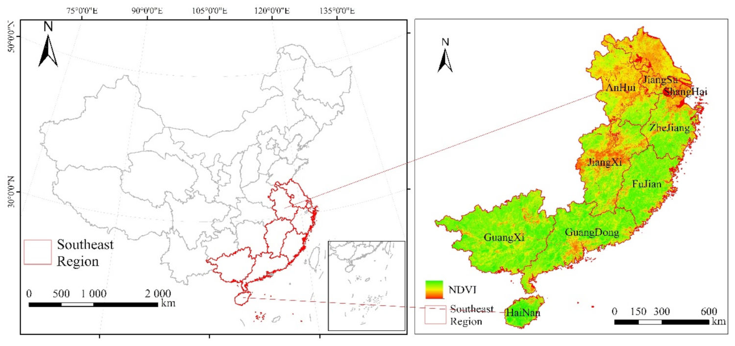
Article

Regression Analysis and Comparison of Economic Parameters with Different Light Index Models under Various Constraints

School of Geoscience and Surveying Engineering, China University of Mining and Technology (Beijing), Beijing 100083, China
*
Author to whom correspondence should be addressed.
Sensors 2021, 21(22), 7561; https://doi.org/10.3390/s21227561
Submission received: 19 October 2021 / Revised: 11 November 2021 / Accepted: 12 November 2021 / Published: 14 November 2021
(This article belongs to the Section Sensing and Imaging)

Abstract

:
Economic globalization is developing more rapidly than ever before. At the same time, economic growth is accompanied by energy consumption and carbon emissions, so it is particularly important to estimate, analyze and evaluate the economy accurately. We compared different nighttime light (NTL) index models with various constraint conditions and analyzed their relationships with economic parameters by linear correlation. In this study, three indices were selected, including original NTL, improved impervious surface index (IISI) and vegetation highlights nighttime-light index (VHNI). In the meantime, all indices were built in a linear regression relationship with gross domestic product (GDP), employed population and power consumption in southeast China. In addition, the correlation coefficient R 2 was used to represent fitting degree. Overall, comparing the regression relationships with GDP of the three indices, VHNI performed best with the value of R 2 at 0.8632. For the employed population and power consumption regression with these three indices, the maximum R 2 of VHNI are 0.8647 and 0.7824 respectively, which are also the best performances in the three indices. For each individual province, the VHNI perform better than NTL and IISI in GDP regression, too. When taking employment population as the regression object, VHNI performs best in Zhejiang and Anhui provinces, but not all provinces. Finally, for power consumption regression, the value of VHNI  R 2 is better than NTL and IISI in every province except Hainan. The results show that, among the indices under different constraint conditions, the linear relationships between VHNI and GDP and power consumption are the strongest under vegetation constraint in southeast China. Therefore, VHNI index can be used for fitting analysis and prediction of economy and power consumption in the future.

1. Introduction

To better understand global change, its causes and its implications, we can relate human activities to natural physical quantities. As an important part of global change, it is necessary to study economic change. Human activity is not simply distributed uniformly across the earth’s surface, but its distribution trajectory is affected by many factors, such as rivers, altitude, light and others. The characteristic of human activities is concentration and aggregation, so it is easy to identify the activity track of human society according to this characteristic. As one of the unique features of human society, light recognition can identify the gathering place of human society.
Nighttime light (NTL) data are used as medium resolution images to explore human social activities [1], such as lighting area [2], population [3,4,5], economy [6,7,8], built area [9], power consumption [10,11], and have achieved good results. The study of the relationship between lighting data, population and gross domestic product (GDP) has also had good results [12,13,14]. At the same time, the relationship between lighting data and population is also tested on a small scale [15]. Therefore, light data can be a good method for socioeconomic estimates. There are two types of nighttime light data most commonly used today, one is the U.S. Air Force’s Defense Meteorological Satellite Program (DMSP) Operational Line Scan System (OLS) and the other one is the Suomi National Polar-Orbiting Partnership (NPP) Visible Infrared Imaging Radiometer Suite (VIIRS) with Day/Night Band (DNB). VIIRS sensor data has higher spatial resolution than DMSP-OLS. What is more remarkable is that VIIRS has a strong ability to amplify low-brightness visible light related to human activities and can observe cities, fishing boats and gas firelight at night without background moonlight [16,17]. Therefore, compared with DMSP-OLS, VIIRS-DNB can provide richer information about human habitation and economic activities [18]. Due to the defects of OLS sensors themselves, night light data in urban centers with high light intensity will show the light saturation phenomenon, that is, DN value increases to a certain extent and does not continue to increase with the increase of ground light intensity.
In view of the shortcomings of traditional studies, Tang et al. took DMSP/OLS light data as the data source, which could better reflect the economic development level of provinces [19]. Using Zimbabwe as the study area, the correlation between total night-time lighting (TNL) and GDP as an indicator, Li et al. compared nighttime lighting images of four regional countries and regional scales in 2000 and 2008, and found that Zimbabwe’s economy declined between 2000 and 2009. Chen. J compared moderate resolution imaging spectroradiometer (MODIS) data with DMSP/OLS and NPP/VIIRS nighttime light data to estimate provincial economic development, and found that, compared with DMSP/OLS nighttime light data, MODIS data improved the accuracy of estimation [20]. In addition, MODIS data are more accurate than DMSP/OLS nighttime light estimates, especially in dark and light-saturated areas, but not as accurate as NPP/VIIRS nighttime light estimates. Taking the U.S. states and metropolitan statistical area for comparison, Chen found VIIRS data in the prediction of cross section is more useful than forecast time series data [21].
Omurakunova studied the effectiveness of night light (NTL), a data source, in monitoring factors related to sustainable development in the Bangladeshi environment [22]. In 2017, Fu put forward the economic index of night lighting (NLEI), and conducted correlation analysis of NLEI and economic indicators of various provinces and cities in China from 1992 to 2012 by using DMSP/OLS data [23]. Qun used the vegetation-adjusted NTL urban light index (VANUI) to alleviate the light overflow problem of DMSP data in big cities. Thus, the dynamic change of urban information systems in China from 1992 to 2009 was estimated. Wei. G utilizes improved impervious surface index, (IISI) estimated the impervious water surface area of arid/semiarid urban areas through linear regression model [24].
It can be seen that the research methods of night light and economy mostly take economy as the index to fit with light data, and most of them are improved in the fitting method. Most of the light indices proposed by scholars, such as IISI and VANUI, focus on impervious water surface and other economy-related studies, without direct and effective studies on the economy itself. Therefore, this paper aims to put forward a light index fitting with the economy and make a comparative analysis with other indices.

2. Materials and Methods

2.1. Study Area

With the exception of Hong Kong, Macao and Taiwan province, China’s major economic regions are also divided in different ways. In addition to their geographical differences, these regions also widely reflect the overall differences in social and economic development. Since the beginning of China’s reform and opening up, southeast China’s natural geographical advantages have led to its rapid economic development. With the introduction of various policies and benefits, southeast China has become the most developed region in China’s economy. The Yangtze River Delta and Pearl River Delta economic zones are the most active regions in China’s economic development. The economic conditions of the southeast region are very good as it hosts Shanghai, China’s economic center and national metropolis, and Shenzhen, a special economic zone in the region. Therefore, this paper chooses the economically and culturally developed southeast region as the research area (Figure 1). The southeast region, located in the southeast of China, includes Jiangsu, Shanghai, Zhejiang, Fujian, Jiangxi, Anhui, Guangdong, Guangxi and Hainan (excluding Sansha City) (Table 1).
Four kinds of data were used in this study, as shown in Table 2, including NPP/VIIRS 2015 annual data [25] and MODIS normalized difference vegetation index (NDVI) data. Administrative boundaries and socioeconomic statistics of provinces, municipalities and prefecture-level cities.

2.2. Data Preprocessing

The VIIRS-DNB data are on a geographic (lat/lon) grid with cell size 15 arc-seconds. With the increase of latitude, the image grid footprint increases. In order to avoid the influence of image grid deformation on nighttime image data and facilitate statistical information, nighttime light images of China’s administrative regions were first extracted. We reprojected the extracted images to the Albers projection and resampled the data to the size of 500 m × 500 m cells using the nearest neighbor algorithm. The annual product was further processed to remove background noise. However, there were still some extremely high light values, such as those of airport lights and power plants. In order to reduce these influences, some studies use the threshold method to remove background information and images [26]. The values for all core areas of the city were below 250 nW cm−2sr−1 because the threshold was set to the maximum, that is, all pixel values over 250 in the study area were reassigned to 250.

2.3. Light Index Model

Considering that the study area is mainland China and there are great differences in land cover types and vegetation coverage among different areas, two types of indices were selected, namely NTL index without other restrictions, and improved impervious surface index (IISI) of weak light area enhanced by logarithm. They can be represented separately by the formula:
N T L = D N B
NTL stands for preprocessed data of VIIRS-DNB, and DNB is the pixel value of the corresponding pixel.
D N B n o r = D N B D N B m i n D N B m a x D N B m i n
where D N B n o r represents the normalized VIIRS-DNB image value range from 0 to 1, D N B m i n is the minimum value and D N B m a x the maximum value, which were 0 and 200, respectively.
I I S I = l o g 2 1 + D N B n o r
where D N B n o r represents normalized VIIRS-DNB value. The logarithm model and coefficient can guarantee an index value between 0 and 1. This index not only suppresses extremely large values but also enhances small ones.
Considering that vegetation has a negative correlation with human activities, that is, the intensity of human nonagricultural activities in the central area of the city is high, and the vegetation coverage is generally less. However, in rural areas, the intensity of human nonagricultural activities is low and vegetation coverage is high. The NTL value of light intensity decreases gradually from the urban center to the outskirts, while the NDVI shows an almost opposite trend. After NTL is normalized to get D N B n o r , it is taken square treatment to achieve the effect of enhancing light intensity.
Due to the nature of the square root function itself, the closer the value of D N B n o r is to 1, that is, the closer it is to the city center, the weaker the enhancement effect is, while the closer the value of D N B n o r is to 0, the farther away from the city center, the stronger the enhancement effect is. When D N B n o r is equal to NDVI and the value of D N B n o r is less than NDVI, which usually occurs in the rural-urban transition area and the countryside far away from the city center, so the D N B n o r is equal to NDVI is taken as the reference. Set the adjustment coefficient of NTL to 1 at this time to achieve the role of light value in the prominent area. When D N B n o r is greater than NDVI, the larger the difference value is, the greater the light intensity is and the closer it is to the active light area. When D N B n o r is less than NDVI, the larger the difference value is, the weaker the light intensity is. Therefore, when D N B n o r is larger than NDVI, the spatial differences of NTL within the region are enhanced, and the adjustment coefficient of NTL is greater than 1. When D N B n o r is less than NDVI, the adjustment coefficient of NTL is set to be less than 1 in order to enhance the difference of light intensity between suburban and rural areas and city center. Based on this idea, the light index shown in Formula (4) is as follows:
V H N I = ( 1 + D N B n o r 1 + N D V I ) N T L
where VHNI is the improved lighting index. Theoretically, when D N B n o r is equal to NDVI, the value of VHNI remains unchanged. When D N B n o r is larger than NDVI, the maximum theoretical value is two times NTL. When D N B n o r is less than NDVI, the maximum theoretical value is 0.5 times NTL. Under the condition of NTL data pretreatment, the calculated VHNI will not have infinite or infinitesimal outliers.
The NTL model is preprocessed light data. Because noise removal and extremely high value elimination will not affect the distribution characteristics of DN value of light data, normalization of NTL will not cause abnormal influence. Therefore, both NTL and D N B n o r can be defined as unrestricted light index.
IISI index is according to Formulas (2) and (3), the normalization processing of lighting data itself only adjusts the range of DN value of lighting data and distributes it in the interval of [0,1]. However, IISI index adopts the logarithm function model. As it is a concave function, the closer the independent variable is to the right range within the scope of definition, the slower the growth rate of the value of the corresponding dependent variable is, the DN value of the light data will be constrained, and the original distribution characteristics and laws will change. Therefore, it is defined as a single light restricted light index.
The vegetation represented by NDVI is added to VHNI, and the lighting type is NTL model, but its adjustment coefficient 1 + D N B n o r 1 + N D V I represents not a simple “non-negative is positive”, but highlights the lighting area or vegetation covered area by comparing the lighting value with vegetation. The appearance of D N B n o r makes the original unrestricted light index (NTL or D N B n o r ) become a single light limiting index. After the introduction of vegetation factor, the adjustment coefficient of NTL becomes complicated, so it is defined as the light limiting index under vegetation constraint.
Firstly, the nighttime light data and NDVI data of China were obtained by using the preprocessed light data and MODIS NDVI data after clipping the administrative boundary of China. Then, the administrative boundary of prefecture-level cities was cut out and processed to obtain the lighting data of three models, and the TNL values of the lighting data of three models in different cities were statistically obtained. The flow chart is shown in Figure 2.

2.4. Rregression Model

We chose four regression models which are the most commonly used in regression analysis to evaluate the potential of nighttime light data for modeling socioeconomic parameters [27,28,29,30,31]: linear regression model (Equation (5)), logarithm regression model (Equation (6)), exponential regression model (Equation (7)), and double logarithm model used for those with small dependent and independent variables (Equation (8)):
P = a T N L X + b
P = a l n T N L X + b
P = a e T N L X
l n P = a l n T N L X + b
P represents social and economic parameters (GDP, power consumption and population), T N L is the total night light intensity of each administrative region (i.e., the sum of all pixel values of light data within the administrative region), T N L X is the total night light intensity of different light index models (NTL, IISI, VHNI).
According to the performance of the four regression models in the overall regression of different indicators in southeast China, which regression model to use in the regression analysis was decided.

3. Result

3.1. Exponential Comparative Analysis

The research area of this paper is the southeast region, where the regional economy is developing rapidly, especially in the provincial capital cities. However, the economic development gap between cities in the study area is still large, there are still some cities in the province lagging behind in economic development. Therefore, in order to understand the relationship between different indices and indicators, the performance of different indices on the same index in different cities was compared. The comparison results are shown in Figure 3, Figure 4 and Figure 5. In Figure 3, Figure 4 and Figure 5, the horizontal coordinate is city, the left ordinate is TNL, and the right ordinate is GDP (100 million yuan), population (ten thousand people) and power consumption (ten thousand KWH). Due to logarithm processing, IISI index has a small value, so it needs to be magnified by 50 times to unify the order of magnitude of the three indicators.
As can be seen from the GDP curve in Figure 3, except Guangdong and Fujian, provincial capitals are all the economic centers in other provinces, making their economies come out on top. Guangdong province, with Guangzhou and Shenzhen as the centers, has developed in parallel. Fujian province’s Fuzhou, Quanzhou two economic development. In the power consumption curve shown in Figure 4, Shanghai has the largest power consumption, while Guangzhou, Shenzhen and Fuzhou have similar power consumption. Except Guangdong province, the capital cities of different provinces have the most power consumption in their own province. Opposite to GDP and power consumption is the population in Figure 5. Shanghai has the largest population and far exceeds that of other cities, while the population of other cities in the same provinces has little difference.
The curve in Figure 3 and Figure 4 shows that the trend of different indices, GDP and power consumption in different cities is basically the same. The values of the three indices in different cities are slightly different and the trend is basically the same. It is worth noting that, compared with GDP, VHNI and NTL are very similar in most cities, but there are quite different values in Hangzhou, Wenzhou, Jinhua, Bozhou, Anqing, Chuzhou, Zhanjiang, Zhaoqing, Wuhu and Huaibei, and the trend is opposite. In comparison with power consumption, the trend of the three indices in Hangzhou and Wuhu is opposite to the actual situation of power consumption, and the trend of the other places is consistent. As can be seen from Figure 5, the population and the three indices have a great contrast among different cities, and the trend is opposite in many places such as Hangzhou, Wuxi, Liuzhou, Huaibei and Bozhou.

3.2. Regression Analysis in General

Taking each city as a part of the whole, linear regression, logarithm regression, exponential regression, and double logarithm regression were carried out for the three indicators. The gross domestic product includes the gross domestic product (including urban population) of prefecture-level cities within each province, in the unit of 100 million yuan. The regression of GDP, population and power consumption of 100 cities in eight provinces and one city in southeast China was carried out through TNL of three light indices. The determination coefficient R 2 of linear, logarithm, exponential and double logarithm model is shown in Table 3. The fitting results of the three indices are shown in Figure 6, Figure 7 and Figure 8.
It can be seen from Table 3 that in the regression analysis of the three indicators of all municipal administrative regions, in the regression analysis of GDP, population and power consumption by linear regression model, the value of R 2 is almost the highest among the four models, except 0.3015 is less than the 0.3059 of the double logarithm in regression of IISI and population. Therefore, for consistency of regression models and strong linear relationship between indicators and indices, only the linear regression model is used for regression analysis below.
In the linear regression analysis results, the index with the best comprehensive performance of the three index fitting results is GDP, and its determination coefficient R 2 is the maximum in the linear fitting of different indices to the same index, which is 0.8466 for NTL, 0.7746 for IISI and 0.8632 for VHNI, respectively. The indicator with the worst fitting performance was the population, and the determination coefficient R 2 was the minimum of the three indicators, which were 0.2488 for NTL, 0.3015 for IISI and 0.2642 for VHNI. In the fitting with GDP as the dependent variable and light index as the independent variable, light index VHNI performed best, R 2 of linear regression was 0.8632, higher than 0.8466 of NTL, and IISI performed worst, R 2 was 0.7746. In the fitting of population size, the linear relationship between TNL and population size of each index is weak, and the value of R 2 is generally low. The R 2 of the three indices is about 0.30, but IISI is more outstanding, for which R 2 is 0.3015, which is greater than the 0.2488 for NTL and 0.2642 for VHNI. In the fitting of power consumption, IISI has the worst performance with R 2 of 0.6404, while VHNI has the best performance with R 2 of 0.7824, which is larger than 0.752 of NTL. As can be seen from Table 3, in the fitting of GDP and power consumption, the determination coefficient R 2 of VHNI has the highest value and the strongest linear relationship, which is greater than the other two indices.
In the case of poor fitting relationship between population quantity and TNL index in southeast China, this paper takes into account social factors in southeast China, the relationship between age and labor force, and uses urban employed population to replace local population quantity as an indicator to make linear regression again. The regression determination coefficient R 2 is shown in Table 4.
By comparing Table 2 and Table 3, it is found that the determination coefficient R 2 of each index is significantly improved after the urban employed population replaces the total population index through linear regression, and the fitting degree is good. The determination coefficient R 2 of VHNI is 0.8647, which is still the best among the three indices. Southeast China has a developed economy, large population and complex structure, and many social factors lead to a large number of idle people. After excluding this factor, urban employment population is used as an indicator for fitting. The linear relationship is shown in Figure 9. The regression coefficient R 2 of NTL index is increased from 0.2488 to 0.8406, and the regression coefficient R 2 of NTL index is increased from 0.2488 to 0.8406. IISI increased from 0.3015 to 0.7509; VHNI increased from 0.2642 to 0.8647. It can be concluded that the linear relationship between lighting index TNL and urban employment population is stronger than the linear relationship between regional population in southeast China. At the same time, in the economically developed southeast region, the linear regression among VHNI with GDP, urban employment population and power consumption at the municipal level is stronger than the other two indices.

3.3. Linear Regression within the Province

Southeast China, with its excellent geographical position, has taken the lead in the surging economic growth of China and become the most developed region in China’s economy. The region includes Jiangsu, Zhejiang, eight other provinces, and one city, Shanghai, whose municipality is directly under the central government. The economic development and industrial layout are different, so the contribution of different industries to GDP, population and power demand cannot be generalized. Shanghai is a municipality directly under the central government and has districts and counties under its jurisdiction, so it does not participate in the linear regression analysis. The three indicators of GDP, population and power consumption of eight provinces are analyzed one by one.

3.3.1. Linear Regression between TNL and GDP

GDP is the GDP of each city in eight provinces, and the unit is 100 million yuan. TNL is the TNL of different indices within the administrative scope of each city. Linear regression is conducted between TNL of three indices in different cities and local GDP, and analysis and comparison are made. The linear regression results of GDP and TNL within each city in the same province are shown in Table 5. The R 2 spatial distribution of TNL and GDP linear regression is shown in Figure 10.
It can be seen from the regression results of the study region that the VHNI index has a better linear regression effect on GDP than the other two indices after regional division by province. Among many provinces, the linearity of GDP and TNL is the strongest in Zhejiang province, followed by Jiangsu and Hainan, and the linearity is weak in Anhui province. In NTL and VHNI indices, Jiangxi and Fujian had the best regression effect, while Anhui had the worst. The value of R 2 of IISI is lower than that of NTL and VHNI in most provinces, but its linear relationship is better than that of NTL and weaker than that of VHNI in Jiangsu and Guangxi. According to the R 2 value of the three indices fitting the municipal GDP divided by province, it can be seen that GDP has the best linear correlation with VHNI index, which is higher than other indices. The provinces with the best fitting degree of VHNI and GDP are Jiangxi and Fujian.
According to the China Urban Statistical Yearbook, the urban greening rates of Jiangxi and Fujian are 44.88% and 42.48% respectively, ranking first among provinces in southeast China, followed by Jiangsu and Zhejiang. In order to further explore the linear regression effect of VHNI and GDP, the regression R 2 is compared with the urban green rate, as shown in Figure 11. From the curve change of R 2 and urban greening rate, the trend of the two is basically the same in different provinces, so there is a certain correlation between them, and the correlation coefficient is 0.4312.

3.3.2. TNL Had a Linear Regression with Urban Employed Population

Considering the abnormal trend of the curves of the three indices and population in Figure 5 in many cities, and the good linear relationship between the urban employed population and TNL shown in Figure 9, the urban employed population was used to replace the number of total population for linear regression, with the unit being ten thousand. The results of linear regression between municipal TNL and the number of urban employed population in the same province are shown in Table 6. The R 2 spatial distribution of TNL and urban employed population linear regression is shown in Figure 12, where UEP is urban employed population.
Results shown in Table 6, compared with the R 2 value in Table 3, replace the index after linear fitting and significantly enhance the decision coefficient R 2 value. The overall fitting precision is greatly increased, further confirmed in the town’s southeastern employment population compared to the local population. The TNL have better linear relation, and the research in this area can provide additional options. For example, in the linear regression of Guangxi province, the R 2 of NTL is 0.8972, the R 2 of IISI is 0.8563 and the R 2 of VHNI is 0.8168. Except for Zhejiang and Anhui, the R 2 of VHNI is the largest in the three indices, and the R 2 of NTL is the largest in the other provinces. Therefore, different from GDP and power consumption as indicators of linear regression, the index with the strongest linear relationship with urban employment population is NTL, followed by VHNI, and the weakest is IISI.

3.3.3. Linear Regression between TNL and Power Consumption

The linear regression results of TNL of the three indices and power consumption are shown in Table 7. The R 2 spatial distribution of TNL and power consumption linear regression is shown in Figure 13, where PC is power consumption.
The regression effect of VHNI and power consumption in Hainan is the best, where R 2 is 0.9483, followed by Guangdong 0.8199, Jiangsu 0.7526 and Zhejiang 0.7196 while Anhui has the worst effect, only 0.4251. IISI index has the worst linear relationship with power consumption, and the overall linear relationship is weaker than VHNI and NTL, except Hainan’s R 2 is 0.9734. The correlation between NTL index and power consumption is between VHNI and NTL.

4. Discussion

In this paper, linear, logarithm and exponential models are compared to perform regression analysis on GDP, population and power consumption. The results show that, among the three models, the linear regression model has the highest correlation with the three indicators. Using the linear regression method, the nighttime light images and three kinds of social and economic statistics of 100 cities in southeast China were analyzed. The lighting data of different cities were obtained by NTL, IISI and VHNI indices, and the TNL and GDP, population and power consumption of each index were divided into overall and provincial scales for linear regression.
In the overall linear regression, TNL of the three indices had a strong linear relationship with GDP and power consumption, and the regression effect was good. By comparing the value of R 2 of the linear regression between the three indices and GDP, VHNI performed best in the regression of the three indices, R 2 was 0.8632, which was higher than NTL 0.8466 and IISI 0.7746. In the linear regression of power consumption, the R 2 of VHNI was 0.7824, which is higher than 0.752 of NTL and 0.6404 of IISI. However, in the linear regression between the index and population, the three indices fitted this index poorly. The R 2 of VHNI, the previous best performer, was only 0.2488, lower than NTL’s 0.2642 and IISI’s 0.3015. Considering the influence of many social factors in southeast China, the R 2 values of the three kinds of index regression were greatly improved after adopting urban employed population instead of regional population as the linear regression index. It shows that the linear relationship between the three indices and urban employment population is much stronger than that of regional population, which can provide an alternative index for future research. Therefore, in the population regression analysis, VHNI had the strongest linear relationship with the three indices.
Among the three linear regression indices using GDP as an indicator, the R 2 value of VHNI in each province was greater than that of NTL and IISI. The regression effect of VHNI in Jiangxi and Fujian was the best, reaching 0.95. The regression effect of VHNI in Anhui was poor, R 2 is only 0.7604. However, it was higher than NTL at 0.6638 and IISI at 0.492. At the same time, it can be seen from the R 2 of linear regression of VHNI and GDP and the curve change of urban green rate that the trend of VHNI and GDP was basically the same in different provinces, so there is a certain correlation between them. The correlation coefficient was 0.4312, which can provide reference for future research. After replacing regional population with urban employment population as regression index, the R 2 of VHNI in Zhejiang was 0.806, and the R 2 of Anhui was 0.852. The R 2 of VHNI was the largest in the three indices of the two provinces, and the R 2 of NTL in the other provinces was the largest. Different from the total regression analysis, NTL replaced VHNI index and became the index with the best linear relationship with urban employment population. In the linear regression experiment with power consumption as an indicator, VHNI was only in Hainan, R 2 was 0.9483, less than the NTL  R 2 of 0.9694, and the other seven provinces all had indices with the best linear relationship with power consumption. Even if R 2 was less than 0.5 in Jiangxi, Fujian and Anhui provinces, it was greater than the other two indices. Therefore, in the provincial analysis, VHNI had the strongest linear relationship with GDP and power consumption.
In summary, the NDVI value in southeast China is high, and the linear relationship between the light limiting index VHNI and the two indicators (GDP and power consumption) under vegetation constraint is the strongest, which is stronger than the unrestricted light index NTL and the single light limiting index IISI. Therefore, in the study area with developed economy and high vegetation coverage, the existing or newly constructed light restriction index under vegetation constraint can be used as the optimal index in the regression study of light index and these two economic statistical parameters, and its effect should be better than the other two types of indices. However, in the same area, if population or population-related statistical parameters are used as indicators for linear regression research, unrestricted light index or single light restricted light index should be used for corresponding research without considering the influence of vegetation. According to the performance of the three indices, VHNI index can be used for regression analysis of GDP and power consumption in the future. Because of VHNI’s good linear relationship with economic and power consumption indicators, it can be used to predict the economy and power consumption. In terms of forecasting power consumption, we can also give relevant opinions on carbon emissions and climate issues.

5. Conclusions

According to the linear regression results of the three indices in the study area, compared with IISI and NTL indices, the newly constructed VHNI index has a better regression effect on regional economy and power consumption both in general and by province, and has broader application prospects. When population is used as an indicator and the overall linear regression is carried out with the regional population, the correlation of the three indices is weak, but when urban employment population is used as a population indicator, the linear relationship between VHNI index and urban employment population is the strongest. The linear relationship between NTL index and regional population was strongest when linear regression was performed by province.
The vegetation information data used by VHNI is the most widely used normalized vegetation index (NDVI). Other vegetation indices, such as enhanced vegetation index (EVI), can reduce the influence of soil background and atmosphere on vegetation index. The ratio vegetation index (RVI), which is sensitive to vegetation in high vegetation coverage area, and the perpendicular vegetation index (PVI), which eliminates the influence of soil background, can be effectively replaced according to the vegetation coverage of the study area. The research area of this paper is southeast China, which is the most economically developed region in China. In the future, the research can be extended to other regions of China and even across the globe for verification. In addition, VHNI is only compared with NTL and IISI in this paper. Other indices can be added in future studies for comparison, analysis and induction, and VHNI can be improved.

Author Contributions

Conceptualization, W.G. and H.J.; methodology, W.G. and H.J.; software, H.J.; validation, H.J. and W.G.; formal analysis, D.Y., X.C., L.W., Z.W. and H.W.; investigation, H.J.; resources, H.J.; data curation, H.J.; writing—original draft preparation, H.J.; writing—review and editing, H.J. and W.G.; visualization, H.J.; supervision, D.Y.; project administration, D.Y.; funding acquisition, D.Y. All authors have read and agreed to the published version of the manuscript.

Funding

This research was funded by National Natural Science Foundation of China, grant number 52174610 and 41930650. The APC was funded by 52174610.

Institutional Review Board Statement

Not applicable.

Informed Consent Statement

Not applicable.

Data Availability Statement

Not applicable.

Conflicts of Interest

The authors declare no conflict of interest.

References

  1. Christopher, N.H.D.; Jan-Peter, M.; Jeremy, G.M. Mapping regional economic activity from night-time light satellite imagery. Ecol. Econ. 2006, 57, 75–92. [Google Scholar] [CrossRef]
  2. Christopher, D.E.; Marc, L.I.; Kimberly, E.B. Night-time lights of the world: 1994–1995. ISPRS J. Photogramm. Remote Sens. 2001, 56, 81–99. [Google Scholar] [CrossRef]
  3. Sutton, P.; Roberts, D.; Elvidge, C.; Baugh, K. Census from Heaven: An estimate of the global human population using night-time satellite imagery. Int. J. Remote Sens. 2001, 22, 3061–3076. [Google Scholar] [CrossRef]
  4. Bailang, Y.; Ting, L.; Yixiu, H. Integration of nighttime light remote sensing images and taxi GPS tracking data for population surface enhancement. Int. J. Geogr. Inf. Sci. 2019, 33, 687–706. [Google Scholar] [CrossRef]
  5. Chu, H.J.; Chenhan, Y. Adaptive Non-Negative Geographically Weighted Regression for Population Density Estimation Based on Nighttime Light. ISPRS Int. J. Geo Inf. 2019, 8, 26. [Google Scholar] [CrossRef] [Green Version]
  6. Noam, L.; Yishai, D. High spatial resolution night-time light images for demographic and socio-economic studies. Remote Sens. Environ. 2012, 119, 1–10. [Google Scholar] [CrossRef]
  7. Mellander, C.; Lobo, J.; Stolarick, K. Night-Time Light Data: A Good Proxy Measure for Economic Activity? J. Cit. Rep. 2015, 10. [Google Scholar] [CrossRef] [Green Version]
  8. Li, X.; Linlin, G.; Xiaoling, C. “Detecting Zimbabwe’s Decadal Economic Decline Using Nighttime Light Imagery”. Remote Sens. 2013, 5, 4551–4570. [Google Scholar] [CrossRef] [Green Version]
  9. Kaifang, S.; Chang, H.; Bailang, Y. Evaluation of NPP-VIIRS night-time light composite data for extracting built-up urban areas. Remote Sens. Lett. 2014, 5, 358–366. [Google Scholar] [CrossRef]
  10. Kaifang, S.; Bailang, Y.; Yixiu, H. “Evaluating the Ability of NPP-VIIRS Nighttime Light Data to Estimate the Gross Domestic Product and the Electric Power consumption of China at Multiple Scales: A Comparison with DMSP-OLS Data”. Remote Sens. 2014, 6, 1705–1724. [Google Scholar] [CrossRef] [Green Version]
  11. Chunyang, H.; Qun, M.; Zhifeng, L.; Qiaofeng, Z. Modeling the spatiotemporal dynamics of electric power consumption in Mainland China using saturation-corrected DMSP/OLS nighttime stable light data. Int. J. Digit. Earth 2014, 7, 993–1014. [Google Scholar] [CrossRef]
  12. Wei, J.; He, G.; Liu, H. Modelling regional socio-economic parameters based on comparison of NPP/VIIRS and DMSP/OLS nighttime light imagery. Remote Sens. 2016, 4, 28–34. [Google Scholar]
  13. Amaral, S.; Câmara, G.; Monteiro, A.M.V. Estimating population and energy consumption in Brazilian Amazonia using DMSP night-time satellite data. Comput. Environ. Urban Syst. 2005, 29, 179–195. [Google Scholar] [CrossRef]
  14. Wu, J.; Wang, Z.; Li, W. Exploring factors affecting the relationship between light consumption and based on DMSP/OLS nighttime satellite imagery. Remote Sens. Environ. 2013, 134, 111–119. [Google Scholar] [CrossRef]
  15. Ma, T.; Zhou, C.H.; Pei, T. Responses of Suomi-NPP VIIRS-derived nighttime lights to socioeconomic activity in China’s cities. Remote Sens. Lett. 2014, 5, 165–174. [Google Scholar] [CrossRef]
  16. Hillger, D.; Kopp, T.; Lee, T.; Lindsey, D. First-Light Imagery from Suomi NPP VIIRS. Bull. Am. Meteorol. Soc. 2013, 94, 1019–1029. [Google Scholar] [CrossRef]
  17. Lee, T.E.; Miller, S.D.; Turk, F.J. The NPOESS VIIRS Day/Night Visible Sensor. Bull. Am. Meteorol. Soc. 2006, 87, 191–199. [Google Scholar] [CrossRef]
  18. Ma, Q.; He, C.; Wu, J. Quantifying spatiotemporal patterns of urban impervious surfaces in China: An improved assessment using nighttime light data. Landsc. Urban Plan. 2014, 130, 36–49. [Google Scholar] [CrossRef]
  19. Tang, L.; Cheng, H.; Qu, G. Estimating Provincial Economic Development Level of China Using DMSP/OLS Nighttime Light Satellite Imagery. AMR 2013, 807–809, 1903–1908. [Google Scholar] [CrossRef]
  20. Chen, J.; Li, L. Regional Economic Activity Derived From MODIS Data: A Comparison With DMSP/OLS and NPP/VIIRS Nighttime Light Data. IEEE J. Sel. Top. Appl. Earth Obs. Remote Sens. 2019, 12, 3067–3077. [Google Scholar] [CrossRef]
  21. Chen, X.; Nordhaus, W.D. VIIRS Nighttime Lights in the Estimation of Cross-Sectional and Time-Series. Remote Sens. 2019, 11, 1057. [Google Scholar] [CrossRef] [Green Version]
  22. Omurakunova, G.; Bao, A.; Xu, W. Expansion of Impervious Surfaces and Their Driving Forces in Highly Urbanized Cities in Kyrgyzstan. J. Environ. Res. Public Health 2020, 17, 362. [Google Scholar] [CrossRef] [Green Version]
  23. Fu, H.; Shao, Z.; Fu, P. The Dynamic Analysis between Urban Nighttime Economy and Urbanization Using the DMSP/OLS Nighttime Light Data in China from 1992 to 2012. Remote Sens. 2017, 9, 416. [Google Scholar] [CrossRef] [Green Version]
  24. Wei, G.; Yuhuan, Z.; Le, G. Using VIIRS-DNB and Landsat data for impervious surface area mapping in an arid/semiarid region. Remote Sens. Lett. 2018, 9, 587–596. [Google Scholar] [CrossRef]
  25. Uprety, S.; Cao, C.; Gu, Y. Improving the Low Light Radiance Calibration of S-NPP VIIRS Day/Night Band in the NOAA Operations. IGARSS 2017. [Google Scholar] [CrossRef]
  26. Jing, X.; Shao, X.; Cao, C. Comparison between the Suomi-NPP Day-Night Band and DMSP-OLS for Correlating Socio-Economic Variables at the Provincial Level in China. Remote Sens. 2016, 8, 17. [Google Scholar] [CrossRef] [Green Version]
  27. Huang, Q.; Yang, Y.; Li, Y.; Gao, B. A Simulation Study on the Urban Population of China Based on Nighttime Light Data Acquired from DMSP/OLS. Sustainability 2016, 8, 521. [Google Scholar] [CrossRef] [Green Version]
  28. Dai, Z.; Hu, Y.; Zhao, G. The Suitability of Different Nighttime Light Data for GDP Estimation at Different Spatial Scales and Regional Levels. Sustainability 2017, 9, 305. [Google Scholar] [CrossRef] [Green Version]
  29. Zhang, G.; Guo, X.; Li, D.; Jiang, B. Evaluating the Potential of LJ1-01 Nighttime Light Data for Modeling Socio-Economic Parameters. Sensors 2019, 19, 1465. [Google Scholar] [CrossRef] [Green Version]
  30. Ji, X.; Li, X.; He, Y.; Liu, X. A Simple Method to Improve Estimates of County-Level Economics in China Using Nighttime Light Data and GDP Growth Rate. ISPRS Int. J. Geo Inf. 2019, 8, 419. [Google Scholar] [CrossRef] [Green Version]
  31. Goldblatt, R.; Heilmann, K.; Vaizman, Y. Can Medium-Resolution Satellite Imagery Measure Economic Activity at Small Geographies? Evidence from Landsat in Vietnam. World Bank Econ. Rev. 2020, 34, 635–653. [Google Scholar] [CrossRef]
Figure 1. Study area including eight southeast provinces and Shanghai. The figure on the left shows the location of the study area and the right figure shows the location image of the study area based on NDVI.
Sensors 21 07561 g001
Figure 2. Flowchart. Comparison of regression analysis between different models and three economic parameters.
Sensors 21 07561 g002
Figure 3. TNL and GDP municipal scale of different indices.
Sensors 21 07561 g003
Figure 4. TNL of different indices and power consumption at municipal level.
Sensors 21 07561 g004
Figure 5. TNL of different indices and population at municipal level.
Sensors 21 07561 g005
Figure 6. (ac) Linear fitting relationships between NTL, IISI, VHNI and GDP, respectively.
Sensors 21 07561 g006
Figure 7. (ac) Linear fitting relationships between NTL, IISI, VHNI and population respectively.
Sensors 21 07561 g007
Figure 8. (ac) Fitting relationships between NTL, IISI, VHNI and power consumption, respectively.
Sensors 21 07561 g008
Figure 9. (ac) Fitting relationships between NTL, IISI, VHNI and urban employed population respectively.
Sensors 21 07561 g009
Figure 10. R 2 spatial distribution of TNL and GDP linear regression.
Sensors 21 07561 g010
Figure 11. Comparison of GDP regression R 2 and urban green rate curve in southeast China.
Sensors 21 07561 g011
Figure 12. R 2 spatial distribution of TNL and urban employed population linear regression.
Sensors 21 07561 g012
Figure 13. R 2 spatial distribution of TNL and power consumption linear regression.
Sensors 21 07561 g013
Table 1. Specific administrative units in the study area.
Serial NumberMunicipality or ProvinceNumber of Cities
1Shanghai1
2JiangSu Province13
3ZheJiang Province11
4FuJian Province9
5GuangDong Province21
6GuangXi Province14
7HaiNan Province3
8AnHui Province16
9JiangXi Province11
Table 2. Data name and source.
Data TypeData Name Data Source
Light dataNPP/VIIRShttps://eogdata.mines.edu/products/vnl/
Vegetation dataMODIS NDVIhttps://modis.gsfc.nasa.gov/
Administrative dataVector of province and city administrative regionHTTP://WWW.NGCC.CN/NGCC/
Socioeconomic statisticsCHINA CITY STATISTICAL YEARBOOKhttp://www.stats.gov.cn/tjsj/ndsj/
Table 3. Three indices versus three indicators in different regression models.
IndexRegression ModelGDPPopulation Power Consumption
NTLLinear0.84660.24880.752
Logarithm 0.57910.24180.2259
Exponential0.50320.24180.2259
Double logarithm0.79940.22590.6453
IISILinear0.77460.30150.6404
Logarithm 0.50610.29850.2985
Exponential0.54170.26150.2615
Double logarithm0.74680.30590.5774
VHNILinear0.86320.26420.7824
Logarithm 0.58850.24630.4741
Exponential0.45920.24440.4979
Double logarithm0.81130.21960.6623
Table 4. The result of linear regression R 2 of different indices TNL on the number of urban employed population.
IndexNumber of Employed People in Urban Areas
NTL0.8406
IISI0.7509
VHNI0.8647
Table 5. Linear regression R 2 of TNL and GDP in each province.
ProvinceNTLIISIVHNI
Zhejiang Province0.91810.90690.9343
Jiangxi Province0.92840.71090.9546
Jiangsu Province0.89580.91580.9375
Hainan Province0.90660.89960.9354
Guangxi Province0.86090.87920.8793
Guangdong Province0.83320.65220.8411
Fujian Province0.91380.8160.9553
Anhui Province0.66380.4920.7604
Table 6. Linear regression R 2 between TNL and urban employed population in each province.
ProvinceNTLIISIVHNI
Zhejiang Province0.79600.77630.806
Jiangxi Province0.85270.77570.8447
Jiangsu Province0.8920.84390.8442
Hainan Province0.87440.8280.8369
Guangxi Province0.89720.85630.8168
Guangdong Province0.83370.5980.8197
Fujian Province0.77680.38680.693
Anhui Province0.84260.83780.852
Table 7. Linear regression R 2 between TNL and power consumption within provinces.
ProvinceNTLIISIVHNI
Zhejiang Province0.68950.68410.7196
Jiangxi Province0.44080.1740.4861
Jiangsu Province0.70570.68960.7526
Hainan Province0.96940.97340.9483
Guangxi Province0.66640.53970.6716
Guangdong Province0.80890.58740.8199
Fujian Province0.30950.11090.4351
Anhui Province0.41510.30320.4251
Publisher’s Note: MDPI stays neutral with regard to jurisdictional claims in published maps and institutional affiliations.

