Author Contributions
Conceptualization, G.D., W.L., G.W., B.W. and M.T.W.; methodology, P.B., V.C., J.D., A.E., J.F., P.K., C.R., U.R., C.T., G.W., B.W., M.T.W. and A.Z.-B.; software, P.B., J.D., J.F., M.I., P.K., C.R., C.T. and A.Z.-B.; validation, P.B., J.D., A.E., P.K., C.R., G.W. and M.T.W.; formal analysis, P.B., J.D., A.E., J.F., M.I., P.K., W.L., C.R., C.T., G.W. and M.T.W.; investigation, P.B., J.D., A.E., J.F., M.I., P.K., W.L., C.R., G.W. and M.T.W.; resources, P.B., R.B., V.C., J.D., G.D., L.D., A.E., J.F., P.F., M.I., P.K., W.L., C.R., M.R., U.R., C.T., G.W., B.W., M.T.W. and A.Z.-B.; data curation, P.B., J.D., A.E., J.F., P.K., W.L., C.R. and G.W.; writing—original draft preparation, P.B., R.B., J.D., W.L. and C.R.; writing—review and editing, P.B., R.B., V.C., J.D., G.D., A.E., J.F., W.L., C.R., U.R., C.T., B.W., M.T.W. and A.Z.-B.; visualization, P.B., R.B., J.D., P.K., C.R. and G.W.; supervision, G.D., W.L. and B.W.; project administration, P.B., J.D., G.D., J.F., W.L., C.R., G.W., B.W. and M.T.W.; funding acquisition, G.D., J.F., W.L., G.W. and B.W. All authors have read and agreed to the published version of the manuscript.
Figure 1.
View of the SAFIR-I detector components.
Figure 1.
View of the SAFIR-I detector components.
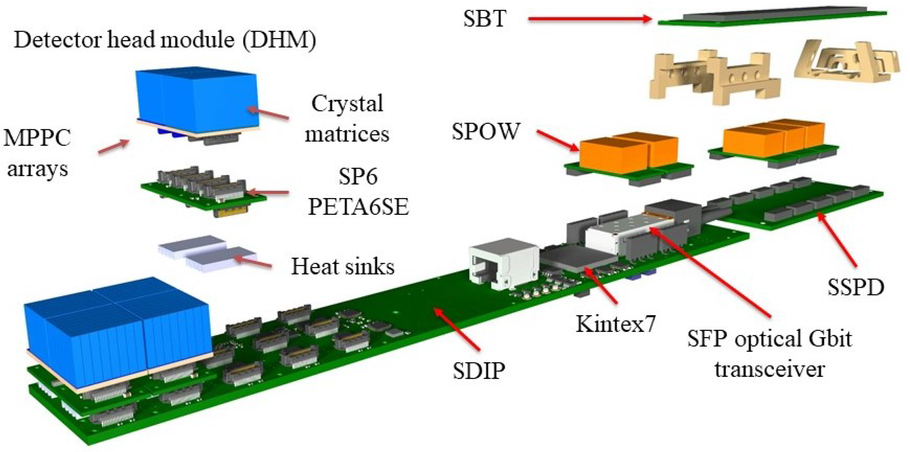
Figure 2.
An exploded view of the casket electronics.
Figure 2.
An exploded view of the casket electronics.
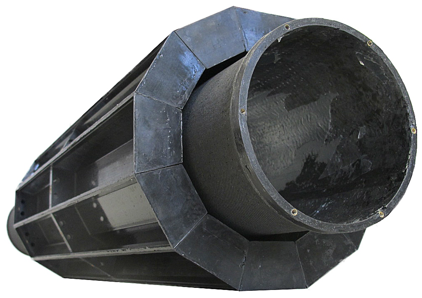
Figure 3.
Carbon fiber structure with inner cylinder and 12 caskets.
Figure 3.
Carbon fiber structure with inner cylinder and 12 caskets.
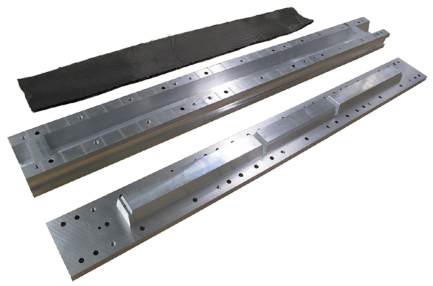
Figure 4.
Casket molding (from the top): Carbon fiber sheets, heatable female mold and male mold.
Figure 4.
Casket molding (from the top): Carbon fiber sheets, heatable female mold and male mold.
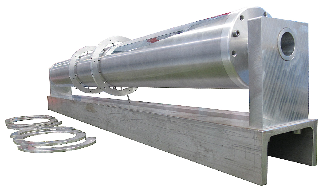
Figure 5.
Mandrel for the fabrication of the inner carbon fiber cylinder.
Figure 5.
Mandrel for the fabrication of the inner carbon fiber cylinder.
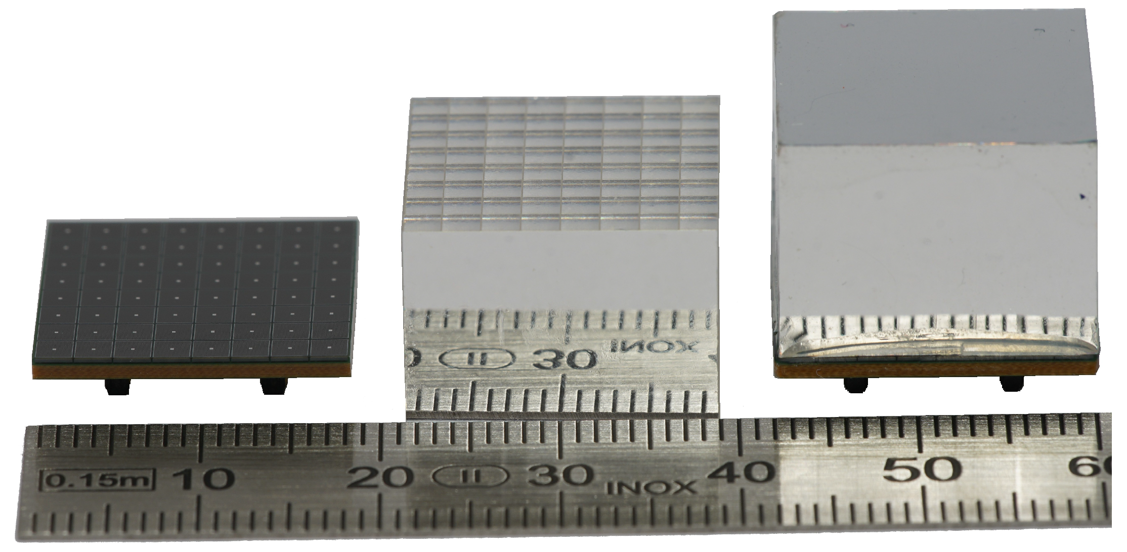
Figure 6.
Image of SAFIR-I’s LYSO crystal assembly. The front reflective foil has been removed from one crystal block to showcase the crystal matrix. Crystal blocks (in the middle) are glued onto 8 × 8 Hamamatsu MPPC arrays (on the left) to form the completed assembly (on the right).
Figure 6.
Image of SAFIR-I’s LYSO crystal assembly. The front reflective foil has been removed from one crystal block to showcase the crystal matrix. Crystal blocks (in the middle) are glued onto 8 × 8 Hamamatsu MPPC arrays (on the left) to form the completed assembly (on the right).
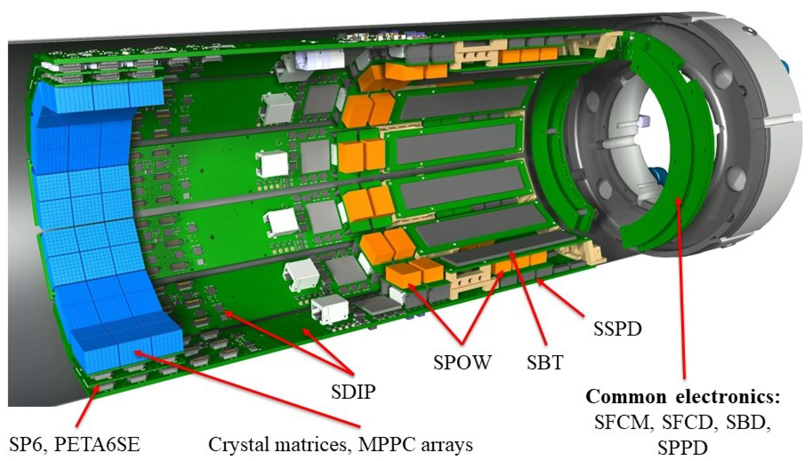
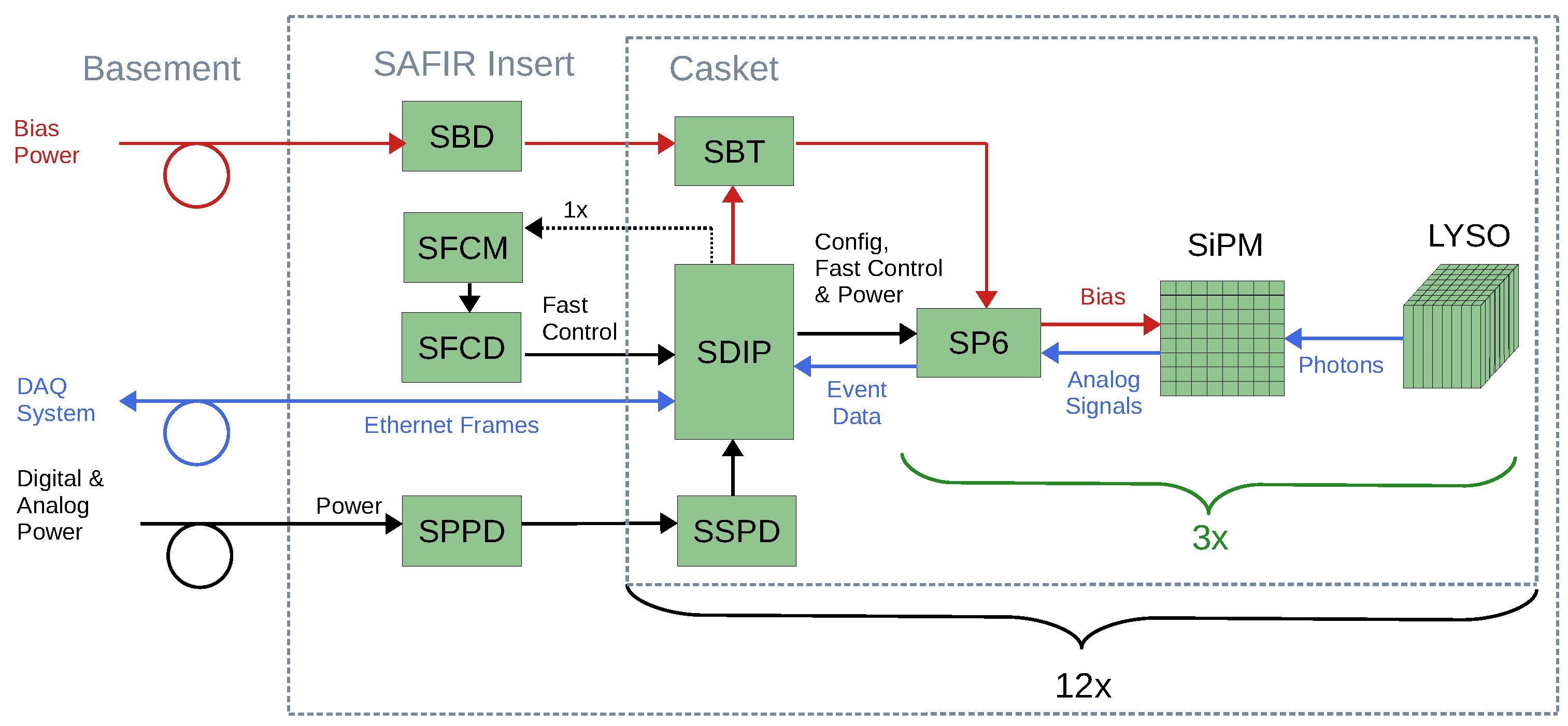
Figure 7.
Schematic depicting the interaction of components within SAFIR-I. Each of the 12 SDIPs supports one SBT and three DHMs, consisting of LYSO scintillation crystals, MPPC SiPM arrays and SP6 PCB’s. These components are all connected to common supporting PCB’s in the detector’s end-flange. Bias, analog and digital power supplies as well as the DAQ system PC are located outside the insert within the service room in the basement.
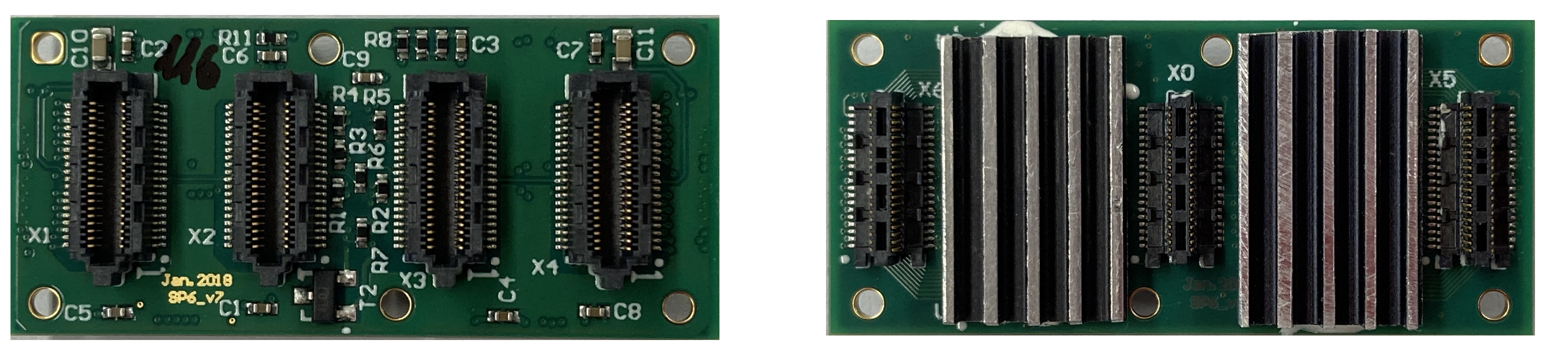
Figure 8.
Image depicting the top and bottom side of the SP6. Four PETA6SE ASICs are located beneath aluminium heat sinks on the bottom side of the PCB, along with three male SAMTEC connectors (ST4-20-1.00-L-D-P-TR) which couple it to the SDIP, while the four female SAMTEC connectors (SS4-20-3.50-L-D-K-TR) on the top side are used to mount the MPPCs.
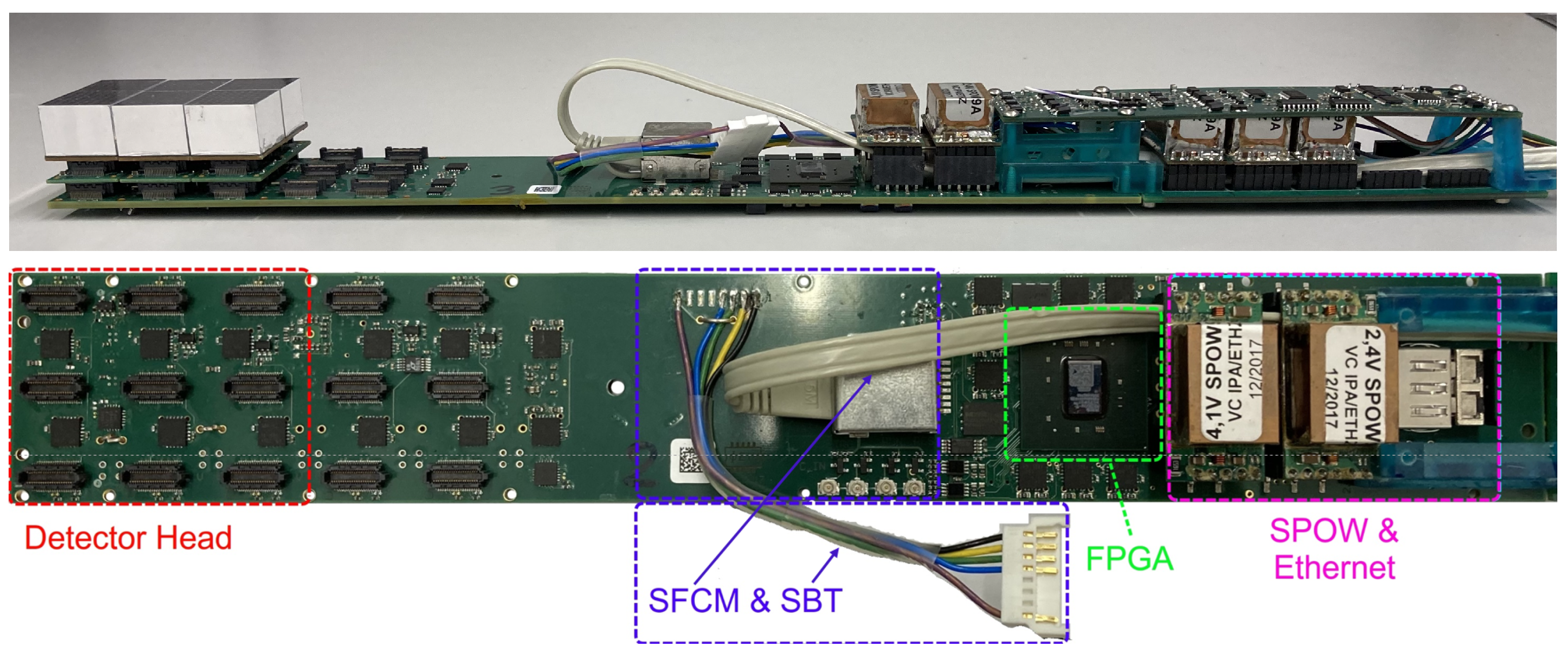
Figure 9.
The SDIP. The upper image depicts the full casket assembly (side view), including the detector head on the left, as well as the SSPD and SBT PCB’s on the right. Below is a birds-eye-view of the SDIP itself. Central component is a Kintex-7 FPGA (marked in green), connected to the DHMs via SAMTEC connectors (red), the SFCM and SBT via cabling (blue), and the DAQ system via an SFP module located under SPOWs (pink).
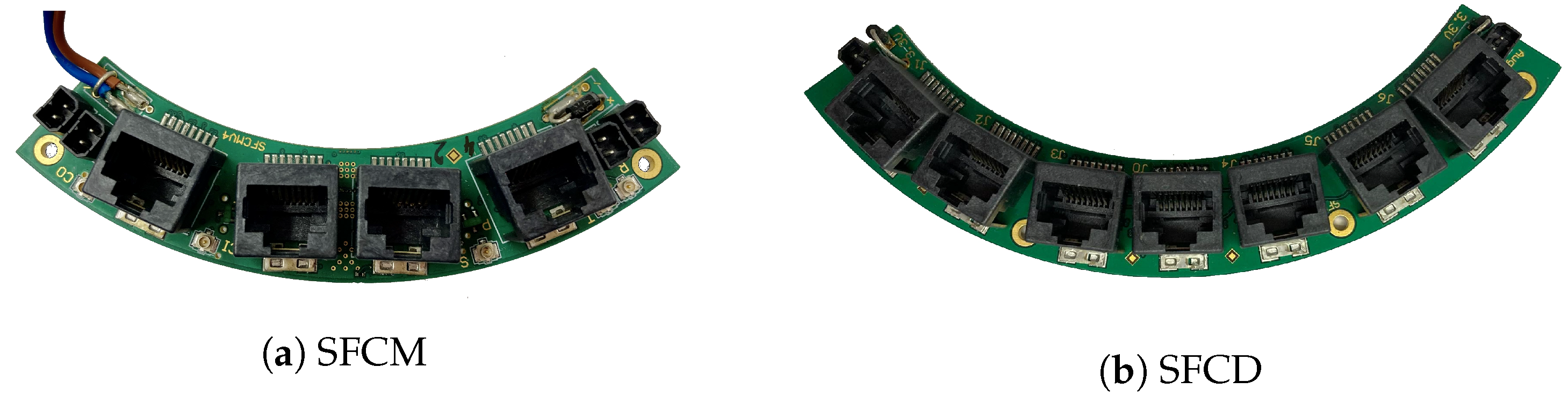
Figure 10.
(a) The SFCM PCB, featuring four RJ45 ports for fast signal distribution. Three coaxial cable connections receive fast signals from a master board, which are distributed to two SFCD PCBs. (b) The SFCD features one input connector in the center and six outputs to distribute the signals from the SFCM to the SDIPs.
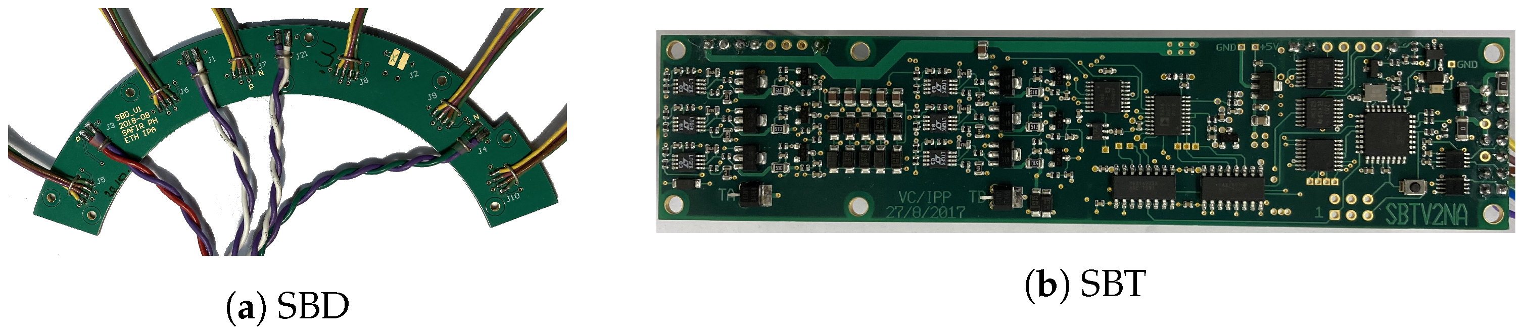
Figure 11.
(a) Starting from the bias power supplies we use two SBDs to supply the required input voltages to all SBTs. The SBDs connects to the bias power supplies via four twisted-pair cables (at the bottom of the image) and serves six SBTs. (b) The SBT regulates up to six bias voltages between −50 V and −60 V.
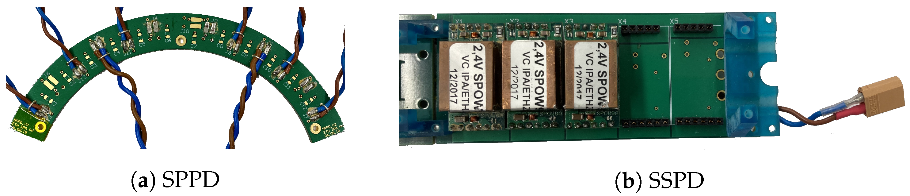
Figure 12.
(a) The SPPD is responsible for distributing the main digital power. Two of these PCBs are part of SAFIR-I, each connecting the external power supply to 6 SSPD PCBs. (b) Each SSPD PCB distributes the digital power from the SPPD to the SDIP.
Figure 12.
(a) The SPPD is responsible for distributing the main digital power. Two of these PCBs are part of SAFIR-I, each connecting the external power supply to 6 SSPD PCBs. (b) Each SSPD PCB distributes the digital power from the SPPD to the SDIP.
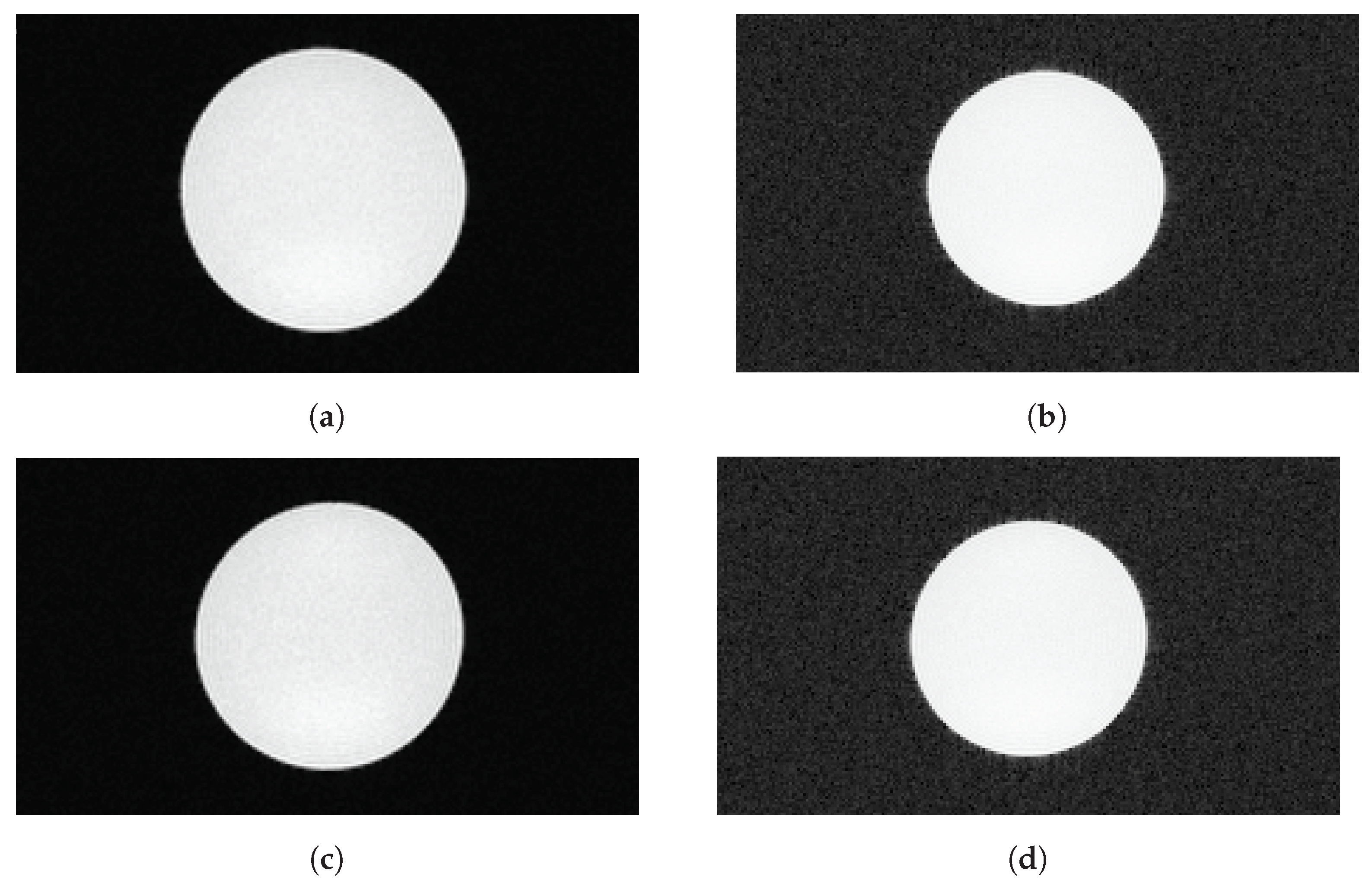
Figure 13.
MR images of a cylindrical water phantom to determine SNR (transverse view). Images taken in parallel to data recording with the SAFIR insert inside the MRI machine during readout at low decay rate (top row) and during the high-rate test (bottom row). (a) Standard image, readout, (b) Modified greyscale version, readout, (c) Standard image, high-rate test, (d) Modified grayscale version, high-rate test.
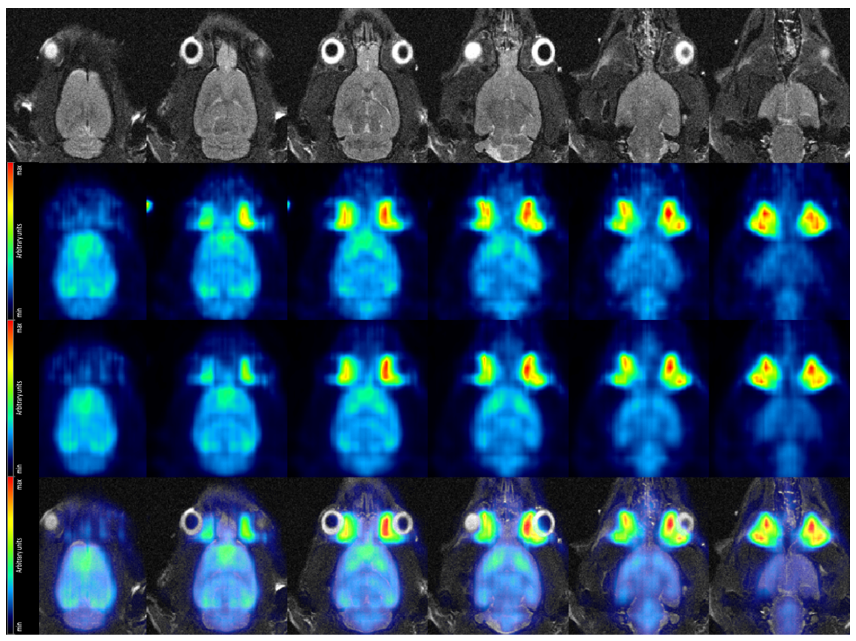
Figure 14.
Coronal view of the rat brain in vivo. (Top row): MR images acquired with a T2-TurboRARE sequence. (Second row): PET data acquired at low dose. Average over frames 22–25, corresponding to 25–45 min after tracer injection. (Third row): PET data acquired at high dose. Average over frames 22–25, corresponding to 25–45 min after tracer injection. (Bottom row) Fused MRI and high dose PET data.
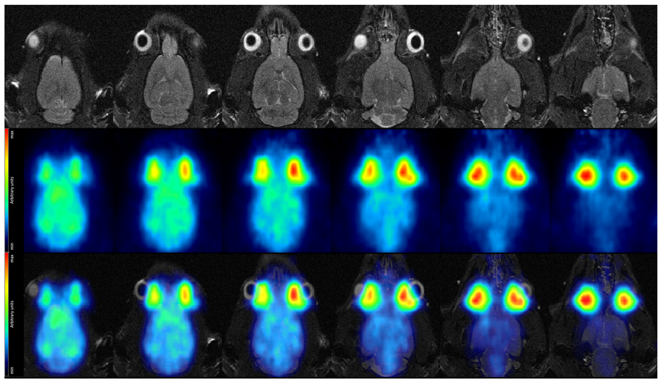
Figure 15.
Coronal view of the rat brain in vivo. (Top row): MR images acquired with a T2-TurboRARE sequence. (Middle row): PET data acquired at high decay rate in a single 5 time frame, recorded 44 after tracer injection. (Bottom row): Fused MRI and high-rate PET data.
Figure 15.
Coronal view of the rat brain in vivo. (Top row): MR images acquired with a T2-TurboRARE sequence. (Middle row): PET data acquired at high decay rate in a single 5 time frame, recorded 44 after tracer injection. (Bottom row): Fused MRI and high-rate PET data.
Table 1.
SNR values observed in baseline and interference measurements (low decay rate).
Table 1.
SNR values observed in baseline and interference measurements (low decay rate).
| Condition | SNR [
] | Deviation from Baseline [%] |
|---|
| Baseline | 2532 ± 6 | – |
| Unpowered | 2622 ± 8 | +3.6 ± 0.4 |
| Powered | 2607 ± 9 | +3.0 ± 0.4 |
| Readout-ready | 2614 ± 14 | +3.2 ± 0.6 |
| Readout | 2623 ± 12 | +3.6 ± 0.5 |
Table 2.
SNR values observed in baseline and interference measurement (high decay rate).
Table 2.
SNR values observed in baseline and interference measurement (high decay rate).
| Condition | SNR [
] | Deviation from Baseline [%] |
|---|
| Baseline | 2502 ± 4 | – |
| High-rate test | 2441 ± 7 | −2.44 ± 0.32 |
Table 3.
CRT, energy resolution and count value (observed coincidences normalized by expected counts, relative to baseline) in low decay rate (365 ) PET data acquisition during simultaneous MRI operation.
Table 3.
CRT, energy resolution and count value (observed coincidences normalized by expected counts, relative to baseline) in low decay rate (365 ) PET data acquisition during simultaneous MRI operation.
| Condition | CRT | Energy Resolution | Count Value |
|---|
| Static B (baseline) | | % | 1 |
| T1-FLASH | | % | |
| T2-TurboRARE | | % | |
| EPI-LR | | % | |
| EPI-HF | | % | |
Table 4.
CRT, energy resolution and count value (observed coincidences normalized by expected counts, relative to baseline) in high decay rate (range 491.7–521.1 MBq) PET data acquisition during simultaneous MRI operation.
Table 4.
CRT, energy resolution and count value (observed coincidences normalized by expected counts, relative to baseline) in high decay rate (range 491.7–521.1 MBq) PET data acquisition during simultaneous MRI operation.
| Condition | CRT | Energy Resolution | Count Value |
|---|
| Static B (baseline) | | %
| 1 |
| T1-FLASH | | % | |
| T2-TurboRARE | | % | |
| EPI-LR | | % | |
| EPI-HF | | % | |
Table 5.
CRT and energy resolution at low and high decay rate with the point and line source, respectively.
Table 5.
CRT and energy resolution at low and high decay rate with the point and line source, respectively.
| Parameter | Low Decay Rate Value | High Decay Rate Value |
|---|
| CRT | | |
| Energy resolution | % | %
|


 ,
, 


