Abstract
In the current industrial landscape, increasingly pervaded by technological innovations, the adoption of optimized strategies for asset management is becoming a critical key success factor. Among the various strategies available, the “Prognostics and Health Management” strategy is able to support maintenance management decisions more accurately, through continuous monitoring of equipment health and “Remaining Useful Life” forecasting. In the present study, convolutional neural network-based deep neural network techniques are investigated for the remaining useful life prediction of a punch tool, whose degradation is caused by working surface deformations during the machining process. Surface deformation is determined using a 3D scanning sensor capable of returning point clouds with micrometric accuracy during the operation of the punching machine, avoiding both downtime and human intervention. The 3D point clouds thus obtained are transformed into bidimensional image-type maps, i.e., maps of depths and normal vectors, to fully exploit the potential of convolutional neural networks for extracting features. Such maps are then processed by comparing 15 genetically optimized architectures with the transfer learning of 19 pretrained models, using a classic machine learning approach, i.e., support vector regression, as a benchmark. The achieved results clearly show that, in this specific case, optimized architectures provide performance far superior (MAPE = 0.058) to that of transfer learning, which, instead, remains at a lower or slightly higher level (MAPE = 0.416) than support vector regression (MAPE = 0.857).
1. Introduction
Over recent years, asset maintenance has received increasing attention in the literature. If considering that appropriate maintenance management has a direct effect on reducing costs and increasing system reliability, availability, and safety [1], it is easy to understand how asset maintenance is a critical success factor in the current industrial revolution 4.0 [2]. More specifically, the adoption of optimized maintenance strategies has been proven to improve tool utilization and productivity, assuring product quality and operational excellence [3].
With the main objective of reducing unexpected breakdowns and possibly catastrophic consequences, maintenance strategies can be roughly classified under [4]: (1) corrective maintenance, (2) preventive maintenance, and (3) prognostics and health management (PHM). In the case of corrective maintenance, machine tools are operated until the tool breaks down, and repairs are made at the time of failure. However, on the other hand, if a critical breakdown occurs, it may cause serious machinery damages. The preventive maintenance aims to prevent the aforementioned problems by scheduling inspection and repair interventions at regular time intervals or operation cycles. In this case, the bigger downside is the waste of time and the replacement costs for components that often are still working. Contrary to previous strategies, PHM relies on the continuous monitoring of equipment health conditions to predict the degradation status, in terms of remaining useful life (RUL), thus supporting more accurate maintenance management decisions.
The prediction of RUL, definable as the “length from the current time to the end of the useful life” as suggested in [5], can be achieved by at least three types of approaches [6]: model-based, data-driven, and hybrid. The model-based approaches (also known as physics-based) refer to mathematical formulations able to model the physical degradation process for the purpose of estimating RUL. In the case of data-driven approaches, instead, RUL is estimated from degradation data collected by monitoring sensors and processed using traditional statistical or machine learning (ML) techniques or even more “advanced” ones based on deep neural networks (DNNs) [7]. However, very often the choice of the appropriate approach depends on the specific problem at hand. Thus, aiming to exploit the strengths of both approaches, data-driven and model-based, they are combined in hybrid approaches by using some kind of fusion scheme [6].
Exploiting the laws of nature to model system degradation, model-based approaches are generally quite accurate. Nevertheless, the implementation of a faithful model for predicting RUL is an expensive and time-consuming process; it may be feasible for simple parts, but may not be for complex components or systems due to the limited understanding of their behavior under all operating conditions. Such disadvantages, combined with the risk of not achieving the desired results, make model-based approaches definitely less attractive than data-driven ones [8].
The various data-driven methods revolve around the processing of features obtained from monitoring sensor data. Consequently, the most important distinction differentiating such methods lies in the way features are obtained, that is, either by traditional handcrafted methods or by learned representations. The methods belonging to the first category utilize representative features, extracted and selected by hand (i.e., handcrafted) on the basis of expert domain knowledge, which are classified or evaluated via regression using appropriate statistical or ML techniques.
The disadvantages of these methods are that handcrafted features are representative only of a specific component or system under certain conditions, while on the other hand, the process of feature extraction and selection is time-consuming and laborious, relying often on strong prior domain knowledge [9]. Moreover, as shown by [10], the performance of ML algorithms is limited by data representation.
In the case of learned representations, on the contrary, representative features of degradation states can be automatically discovered from sensor data by using deep learning (DL) techniques [7,11]. Up to now, a lot of fruitful research results involving many different fields, ranging from image recognition to natural language processing, have been reported in the DL literature [12]. Although, recently, an increasing number of research studies exploiting DL has appeared in the RUL literature, there is still less availability of optimized DL models and architectures compared to other fields.
In the present study, a new DL model based on a convolutional neural network (CNN) is proposed for the RUL prediction of punching tools. The main contributions are (i) representation of punch deformation with depth and normal vector maps (DNVMs) obtained from 3D scan point clouds; (ii) CNN-based RUL prediction with network architecture optimized using genetic algorithm (GA); (iii) validation of the proposed method with real data sets representing three different deformation modes.
2. Related Works
Complex real-world data are very useful in many machine-learning applications, including RUL prediction, but they are also cumbersome to process, transmit and store, due to their high-dimensional nature. More effective and low-dimensional features can be obtained from high-dimensional data by using representation learning techniques. The year 2006 marked an important turning point in this research area, since earlier widely used methods such as principal component analysis (PCA) [13,14] and linear discriminant analysis (LDA) [15] gave way to more advanced DL methods [16]. DL architectures, in contrast to shallow ones, are composed of multiple data transformation layers, providing higher hierarchical abstraction levels, and are thus more useful for classification, detection and prediction tasks.
One of the most common DL approach is the stacked sparse auto-encoder (SAE), in which a network of multiple encoder layers is used to transform high-dimensional data into low-dimensional features and, conversely, a network of multiple decoder layers recovers the original data. Specifically, the RUL of an aircraft engine was predicted by Ma et al. [17] by using SAE to extract performance degradation features. Sun et al. [18] addressed the problem of deep transfer learning with SAE networks for predicting the RUL of a cutting tool. They investigated three different transfer strategies, i.e., weight transfer, feature transfer, and weight update, to transfer a trained SAE to a new object tool under operation without providing supervised training information. The authors claimed that deep transfer learning improves performance of RUL prediction also in the case of little historical failure data for training. Ren at al. [19] proposed a DL-based framework for bearing RUL prediction using deep auto-encoder (DAE) and time-frequency-wavelet joint features to represent the bearing degradation process. As the authors pointed out, the advantages offered by the deep autoencoder method were twofold, i.e., automatic feature selection and over fitting problem prevention thanks to reducing network parameters.
Another neural network class arousing considerable research interest in feature learning is represented by the restricted Boltzmann machine (RBM). It is an energy-based neural network with two layers of stochastic binary neurons, one is the visible layer and the other one is the hidden layer. The main issues when dealing with RBMs (even stacked in multiple layers) is the model parameter initialization (e.g., learning rate, momentum, number of hidden units, mini-batch size, etc.) and how to regularize the model to avoid overfitting and improve the learning process. Liao et al. [20] addressed the regularization problem by suggesting a new term allowing an RBM to be trained to output a feature space that better represents degradation patterns in RUL prediction. Although one RBM layer was used, they pointed out that their method can be extended by stacking multiple RBM layers in a deeper neural network architecture.
Haris et al. [21] addressed the problem of finding optimal hyperparameters for a deep belief network (DBN), which is a generative model composed of multiple RMB layers, with the purpose of predicting the RUL of supercapacitors. To this end, they proposed a combination of Bayesian and HyperBand optimization and showed the universality of their model by training it on different degradation profiles with the same hyperparameters.
Aiming to predict the RUL of a complex engineering system whose malfunctions may be caused by multiple faults, Jiao et al. [22] proposed a RUL prediction framework for multiple fault modes consisting of three main modules: DBN-based extraction of degradation features where original data were preprocessed with a gap metric, fault identification under multiple fault conditions via support vector data description (SVDD) monitoring, RUL estimation via the particle filter (PF) and adaptive failure threshold.
Ma et al. [23] assessed the health condition of a bearing rig by using a discriminative DBN model composed of four layers. They obtained the model parameters, i.e., the number of neurons of the two hidden layers and the learning rate, by using the ant colony optimization (ACO) algorithm. The data consisted of vibration signals collected at 10 min intervals with a sampling frequency of 10 kHz. The degradation prediction was formulated as a classification problem with five classes representing the bearing conditions during the evolution process.
Zhang et al. [24] proposed a DBN-based ensemble method for RUL prediction in which multiple DBNs were evolved using a multi-objective evolutionary algorithm integrated with the traditional DBN training technique. They used DBNs with three hidden layers, whose optimization parameters were the number of neurons, the weight cost, and learning rates. They evaluated their method on the turbofan engine degradation problem provided by NASA, i.e., the Commercial Modular Aero-Propulsion System Simulation (C-MAPSS) data sets [25], composed of multivariate temporal data coming from 21 sensors.
Another DL model recently investigated in RUL prediction is the CNN [26], a type of multi-layer feed-forward network originally conceived to recognize visual patterns from images [27], whose feature learning capabilities are enabled through the combination of multiple convolution and pooling layers. Babu et al. [28] reported the first attempt of predicting RUL using CNN-based feature learning combined with linear regression from multi-channel time series data. As the authors pointed out, the multiple layers composing the DL architecture effectively learned local salience representations of multi-channel signals (provided as two-dimensional input) also in different scales. They showed good RUL estimation performance on two publicly available data sets, the NASA C-MAPSS data set and the PHM 2008 Data Challenge data set [29].
Since sensor data involved in RUL estimation are traditionally arranged in a time-series form, either uni- or multi-variate, the use of recurrent neural networks (RNNs) has been suggested to better deal with the sequential nature of these data [30]. However, as it is well-known, RNNs suffer from a vanishing/exploding gradient in the presence of long-term time dependency. To overcome this drawback, Zheng et al. [31] suggested that the RUL be estimated with a long short-term memory (LSTM) network, which is a type of RNN able to effectively model sequential data, without suffering from long-term time dependency problems. To validate their LSTM model for RUL estimation, they used the C-MAPSS data Set, the PHM 2008 Challenge data set, and the Milling data set.
Aiming to exploit the power of CNN to learn discriminative features from two-dimensional inputs, Li et al. [32] proposed a CNN deep learning architecture based on a time window approach able to handle multi-variate temporal information. To validate the effectiveness of their approach, they estimated the RUL of aero-engines using the NASA C-MAPSS data set. The achieved prediction performance was significantly better than the CNN approach presented by Babu et al. [28] and was also comparable with the LSTM approach of Malhotra et al. [33], but employing simpler architecture and lower computing load.
The approaches reviewed so far receive a time series of sensor data as input (e.g., vibration signals, engine data, physical properties, etc.), usually organized as 1D arrays, but often also as 2D arrays in the case of multi-channel data (i.e., multivariate time series). A special case of 2D representation is image data, traditionally used for visual inspection to assess component or system conditions. Recently, image data were used to automatically predict fault or degradation of machine components, with better results for larger data sets [34].
Since large data sets are not always available within PHM applications, the problem of insufficient images for training CNN models has been addressed through transfer learning by Marei et al. [35], using microscope images of a cutting tool flank. Essentially, transfer learning allows knowledge acquired from a similar or different domain to be reused in a new domain. In practice, DL models pretrained on large general-purpose image data sets (e.g., ImageNet [36], ILSVRC: ImageNet Large Scale Visual Recognition Challenge [37], CIFAR-10/CIFAR-100 [38], and so on) can be fine-tuned using available image data to perform predictions on new problems. However, the underlying assumption for transfer learning to work well is that the feature distributions across the two domains are the same.
DL models require an accurate setting of multiple DNN architectural parameters, which is a time-consuming and experience-intensive task. The parameter setting problem has been tackled by Mo et al. [39], adopting an evolutionary algorithm to find the optimal parameter configuration. Furthermore, they proposed a multi-head CNN structure followed by a LSTM network, pointing out the superiority of multi-head CNN models over single-head multi-channel ones, since the former keep the extracted features separate whereas the latter mix them all together losing specialized features. They demonstrated the effectiveness of their solution using time series data from the NASA C-MAPSS data set.
In real-world settings, the collection of machinery health information might be challenging due to some kind of restrictions (e.g., small component size and narrow camera field-of-view, component partially hidden inside the machine, and so on), giving rise to partial or incomplete data. This problem, referred to as the partial observation problem, has been addressed by Li et al. [40] presenting a supervised attention mechanism for feature learning based on CNN and LSTM, followed by a regression layer for estimating the RUL of an industrial cutting wheel from images.
3. Materials and Methods
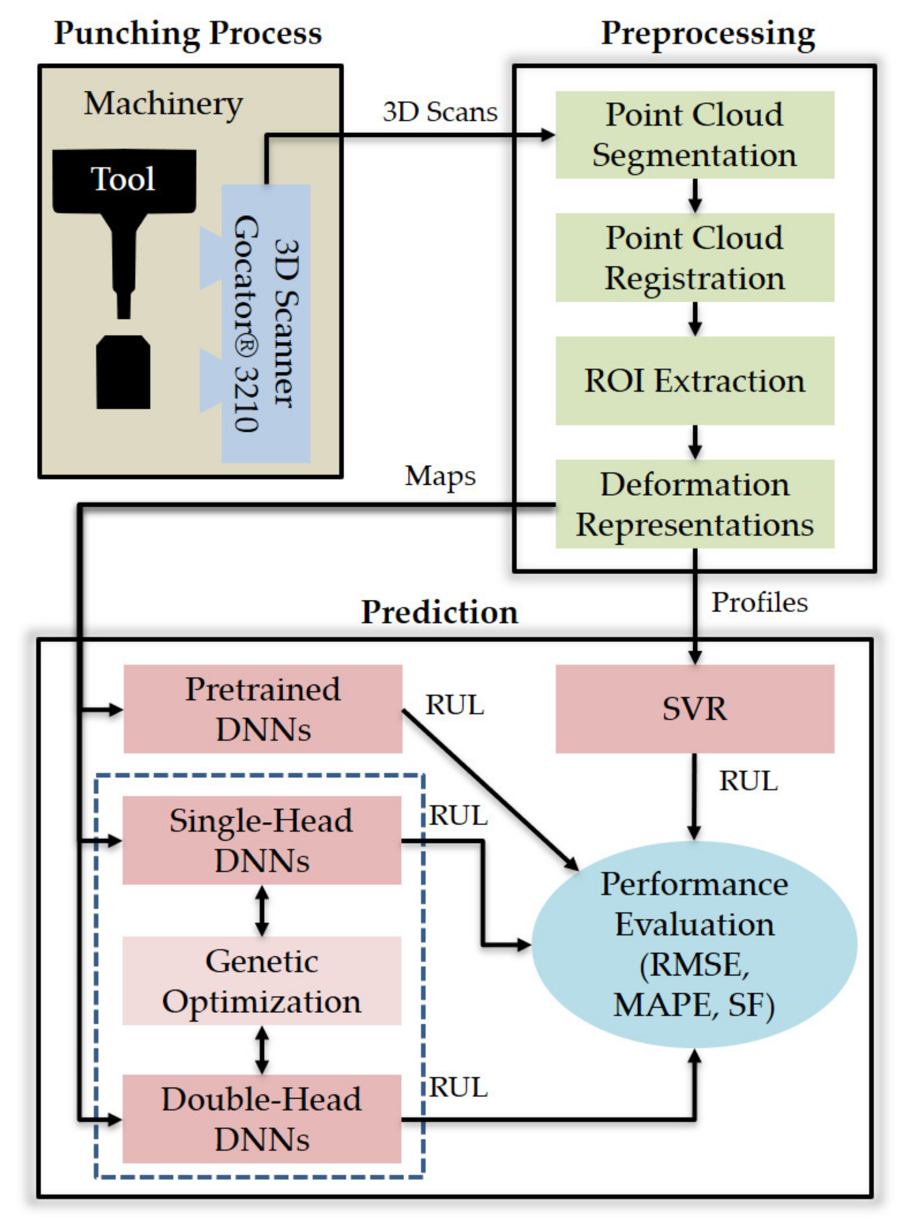
This section details the materials and methods used in this study to predict the RUL of a punch tool from 3D scan data. More specifically, the next subsections deal with the following aspects: (1) the data acquisition system and experimental setup, (2) the 3D scanning process (i.e., pre-processing of 3D point clouds and feature extraction), (3) the adopted metrics to evaluate RUL prediction performance, (4) the DNN architectures generated by genetic optimization, (5) the genetic optimization technique, and (6) the support vector regression (SVR) approach used as classic ML benchmark. The overview of this research is provided in Figure 1, the components of which are detailed in the following subsections.
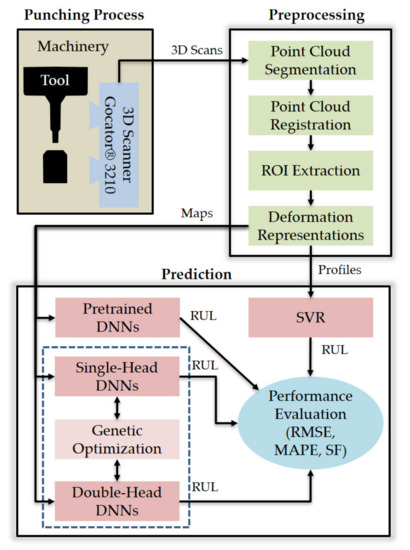
Figure 1.
Overview of this research.
3.1. Experimental Setup and Data Acquisitions
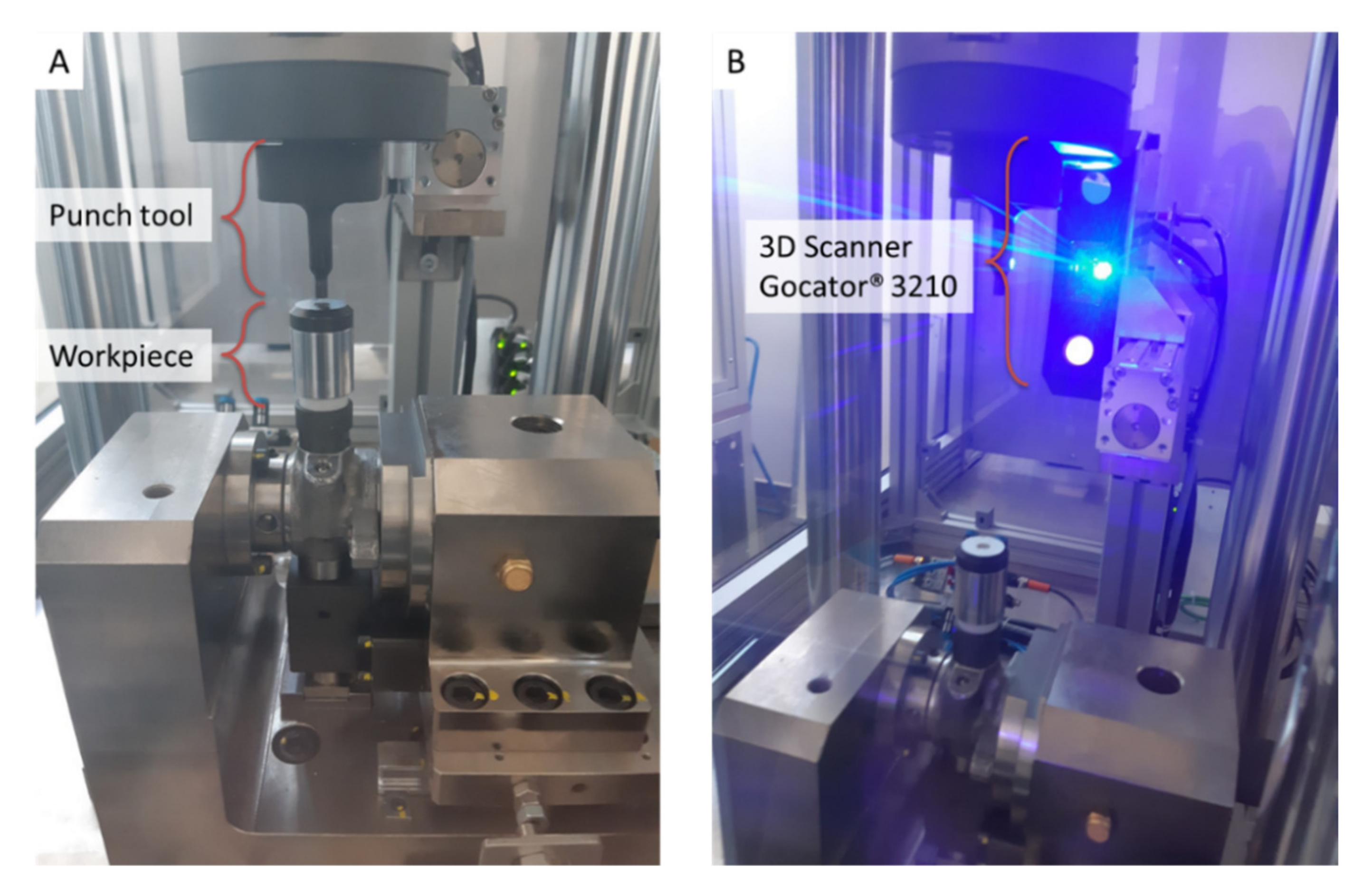
The present study focuses on RUL prediction of punch tools mounted on a punching machine, such as the one shown in Figure 2, used to process pump workpieces by making a punch on their upper end. The RUL prediction is based on 3D scan data acquired by a Gocator® 3210 (LMI Technologies Inc., Burnaby, BC, Canada) [41] sensor, tightly clamped on the punching machine structure (Figure 2B). The 3D scan sensor, equipped with a stereo camera of two megapixels and a blue LED projector, provides 3D point clouds in a single snapshot for accurate noncontact measurements down to 35 μm.

Figure 2.
Punching machinery: (A) punch tool and pump workpiece, (B) Gocator® 3210 3D scanning sensor.
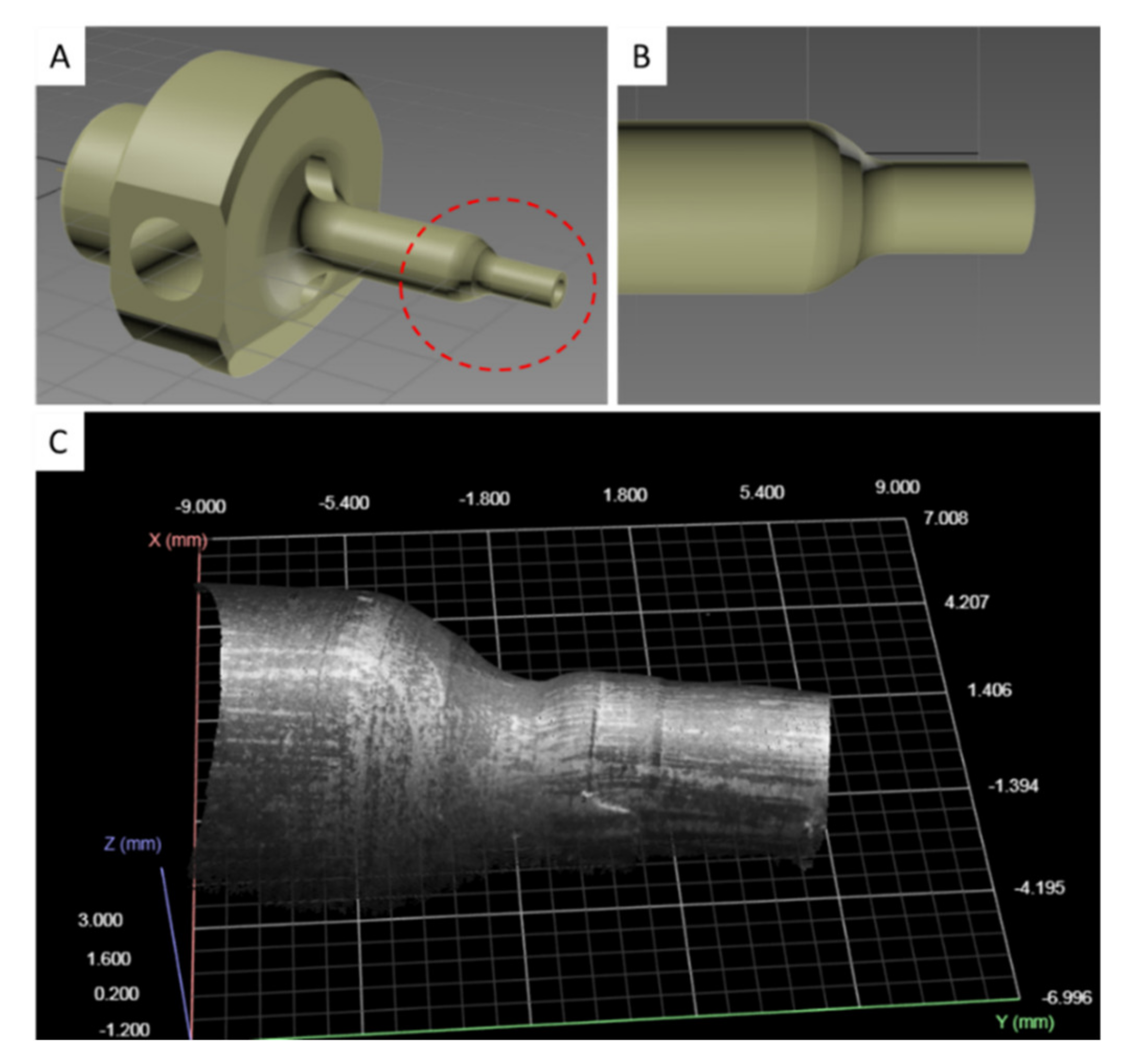
The punch tool consists of two cylindrical ends, of which the one having a larger diameter serves to clamp it to the machine, while the other is the working region. The 3D model of the punch tool is provided in Figure 3, in which the working region is highlighted by a dashed red line (Figure 3A). During the machining cycles, the working surface of the punch (Figure 3B) undergoes progressive deformations (Figure 3C). Three-dimensional scans of these surface deformations, suitably processed using ML algorithms, can be exploited to predict the RUL of the punch tool.
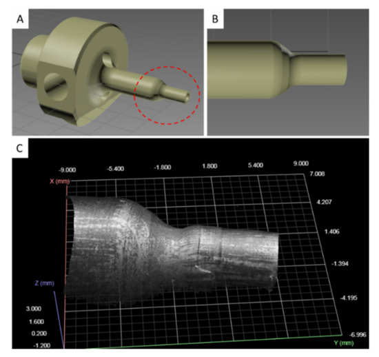
Figure 3.
Punch tool 3D model. (A) Full view of the punch tool with working region circled with a dashed red line. (B) Detail of the working region. (C) 3D point cloud with grayscale patches of the working region obtained from a 3D scan snapshot.
During the experimentation phase, three identical punch tools were brought to the end of their life cycle, subjecting them to different loads. The first punch tool, P1, was operated with an incremental load ranging from a minimum of 10 kN to a maximum of 15 kN, obtaining a total of 714 scans performed every 50 pressing cycles. The second punch tool, P2, was tested with an incremental load ranging from 20 to 28 kN, for a total of 521 scans performed every 60 pressing cycles. The third punch, P3, was subjected to an incremental load ranging from 15 to 20 kN, generating a total of 779 scans captured every 50 pressing cycles. In such a way, a total number of 2014 scans was produced in approximately six months.
3.2. D Scan Preprocessing
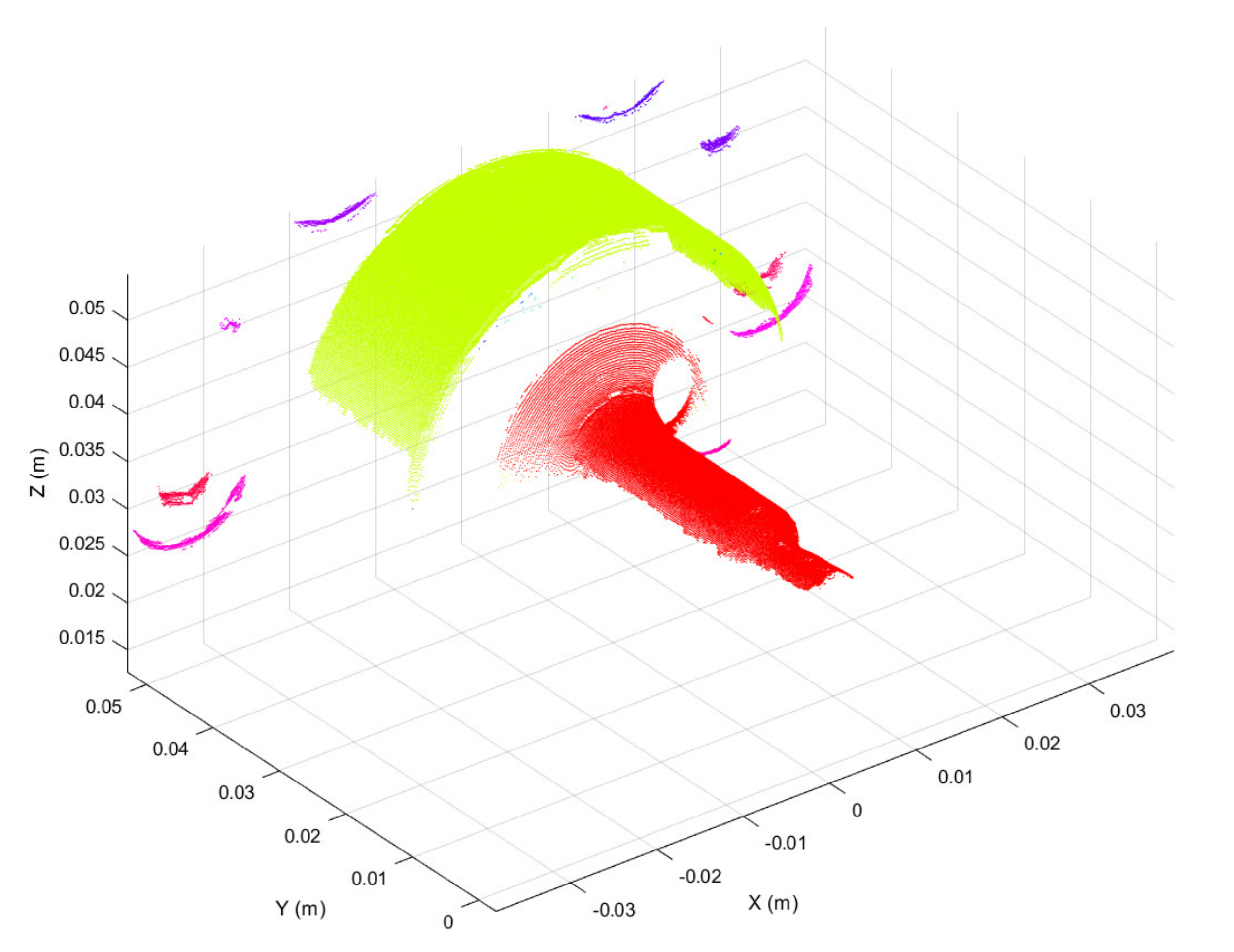
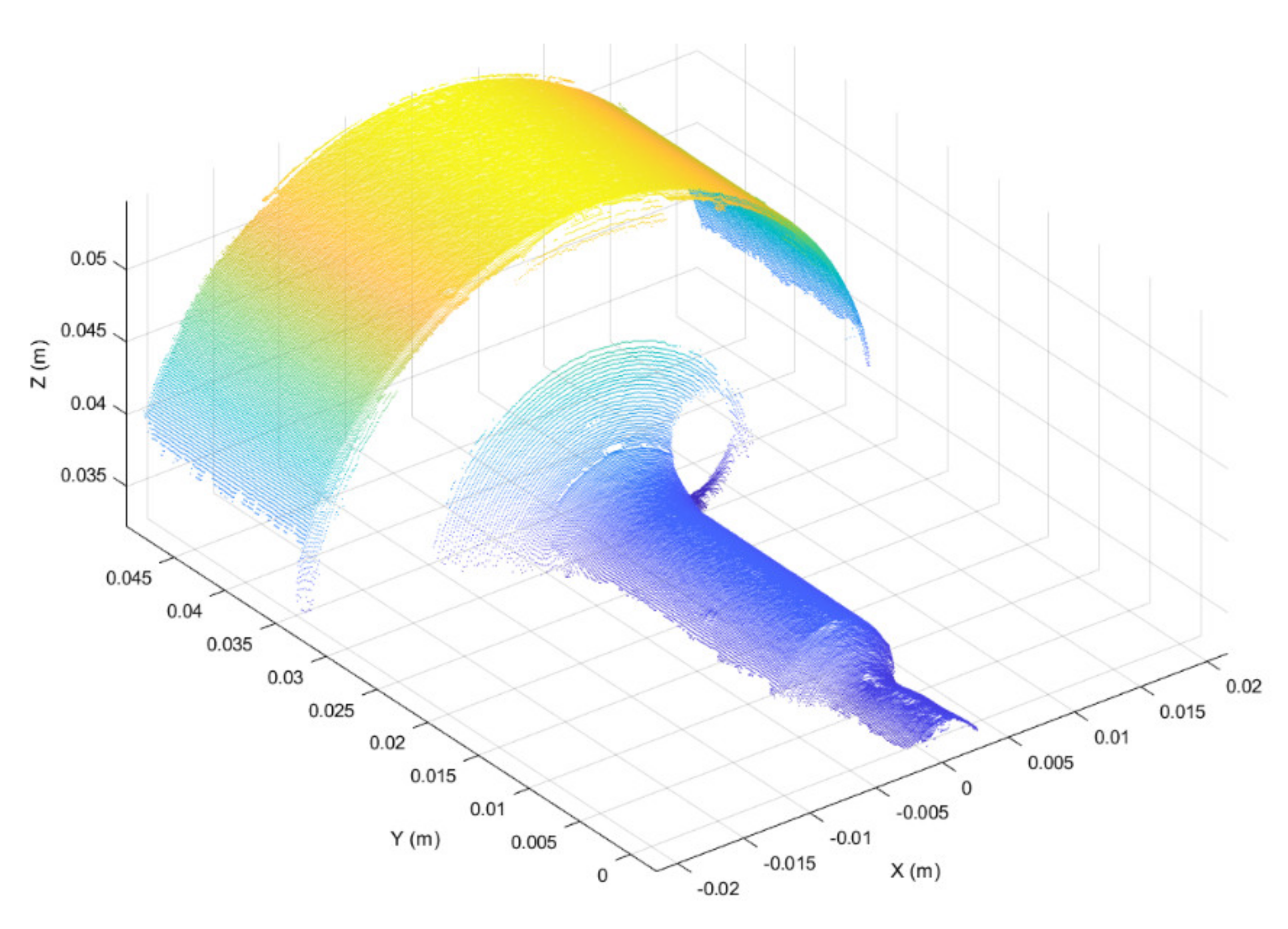
Three-dimensional scans obtained as discussed above were preprocessed in the form of 3D point clouds. Due to reflections from the metallic surface, raw 3D point clouds may be corrupted by artefacts, i.e., spurious 3D points. To overcome this issue, the first preprocessing step was to segment each raw point cloud into clusters, considering a minimum Euclidean distance between 3D points from different clusters, as represented in Figure 4. Then, the clusters were filtered based on the number of 3D points, keeping the two clusters with the greater number of points. The resulting 3D point cloud, provided in Figure 5, is composed of two main segments. The points located at y < 0.01 form the working surface, whereas those located at y > 0.03 represent the so-called best-fit surface used in the following step for point cloud registration. Although the 3D scan system is firmly clamped to the machine structure, continuous vibrations can produce slight misalignments between 3D point clouds. A rigid registration step was utilized to correct such misalignments.

Figure 4.
3D point cloud segmented using the Euclidean distance between 3D points from different clusters. Segmented clusters are represented in different colors.

Figure 5.
Filtered 3D point cloud after segmentation. Two main segments are visible.
The semi-cylindrical surface with the largest diameter, shown in Figure 5 (i.e., 3D points with y > 0.03), was used as the best-fit reference surface for registration, since this surface was the least subject to deformation during punching operations. The iterative-closest-point (ICP) algorithm, originally suggested by Besl and McKay [42], was used to register the best-fit surfaces of segmented point clouds.
Substantially, the ICP algorithm is an optimization process whose main goal is to find the best local (in a least-square sense) rigid transformation by means of singular value decomposition (SVD) [43]. More specifically, the iterative process consists of the following main steps: (1) projection of the two point clouds under registration, (2) estimation of the optimal rigid transformation via SVD, (3) application of the transformation to a subset of randomly selected points, (4) evaluation of the alignment via least median estimator [44], (5) if the alignment error is smaller than a prefixed threshold, the rigid transformation is applied to all the point clouds, otherwise, the above steps are repeated. The pseudocode of the registration procedure is reported in Algorithm 1.
| Algorithm 1. Point cloud registration | |
| 1. | ;//Reference point cloud |
| 2. | ;//Data point cloud to be registered () |
| 3. | //Tolerance between consecutive iterations |
| 4. | ;//Maximum number of iterations |
| 5. | for |
| 6. | ; //Normalization of |
| 7. | end for |
| 8. | for ; ; |
| 9. | ;//Matching subset (from now ) |
| 10. | for |
| 11. | ; //Normalization of |
| 12. | end for |
| 13. | Calculate the SVD decomposition of the matrix ; |
| 14. | ;//Rotation matrix |
| 15. | ;//Translation matrix |
| 16. | if //Termination condition |
| 17. | break; |
| 18. | end if |
| 19. | end for |
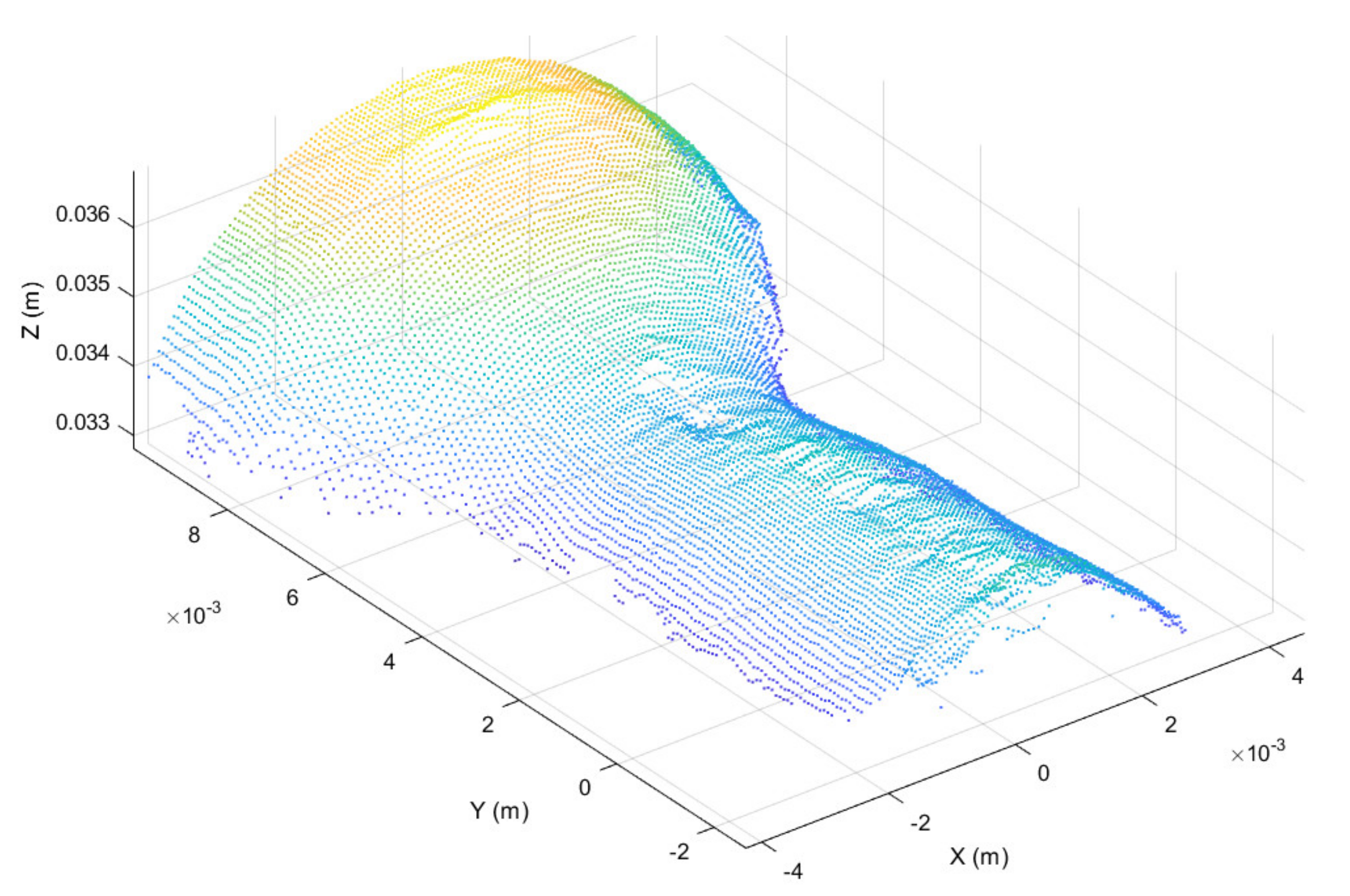
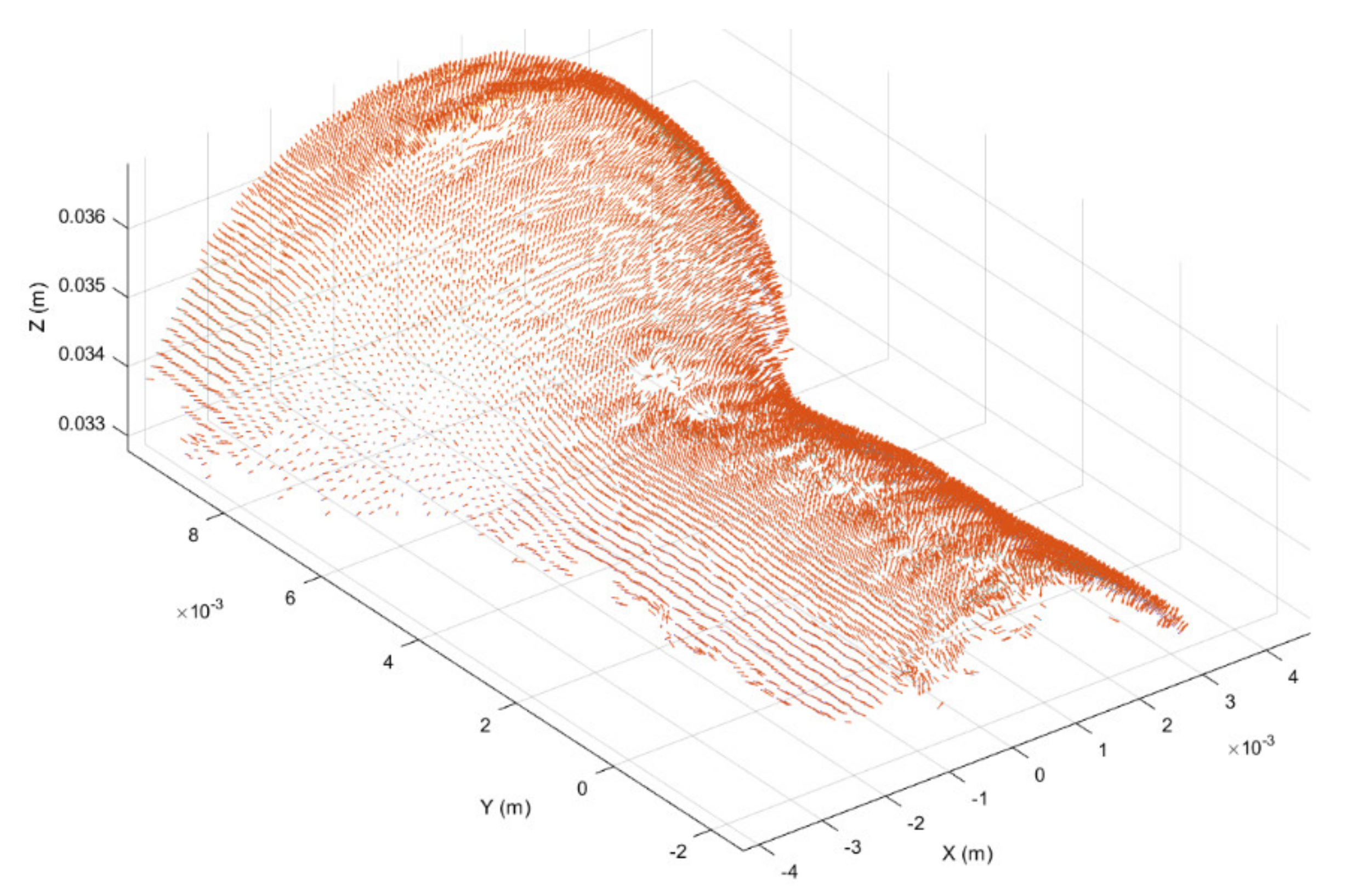
Once registered, the point cloud was cropped to take only the working region, thus highlighting the surface deformation, as shown in Figure 6. In addition, in order to further highlight the working surface deformations, for each point belonging to the cropped point cloud the surface normal vector was considered [45], obtaining the normal representation shown in Figure 7.

Figure 6.
Working surface cropped from registered point cloud.
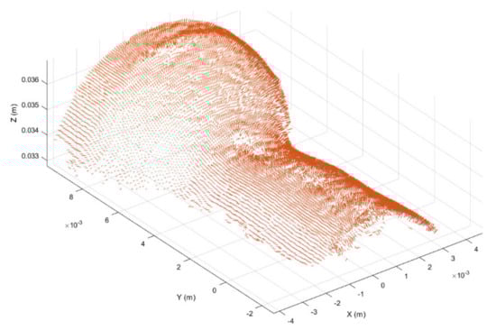
Figure 7.
Surface normal vector representation of the working region obtained from the cropped point cloud provided in Figure 6.
To exploit most of the DNN feature extraction capabilities, depth and normal vector representations were transformed into two-dimensional maps, reported in Figure 8, i.e., depth map (Figure 8A) and normal vector map or normal map (Figure 8B), respectively.
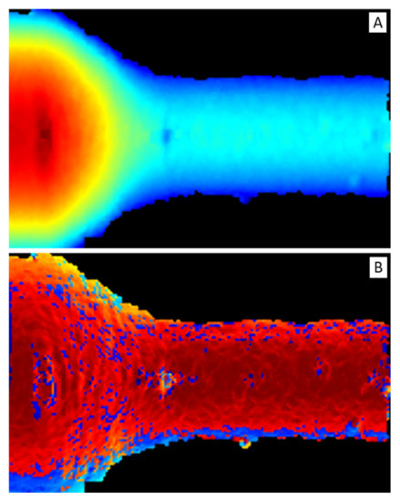
Figure 8.
(A) Depth map. It is a false-color image: red color represents short distances and blue long ones. (B) Normal map. It is a false-color image: dark-red color represents vectors parallel to z-axis (i.e., pointing out of the image plane) and light-blue perpendicular ones.
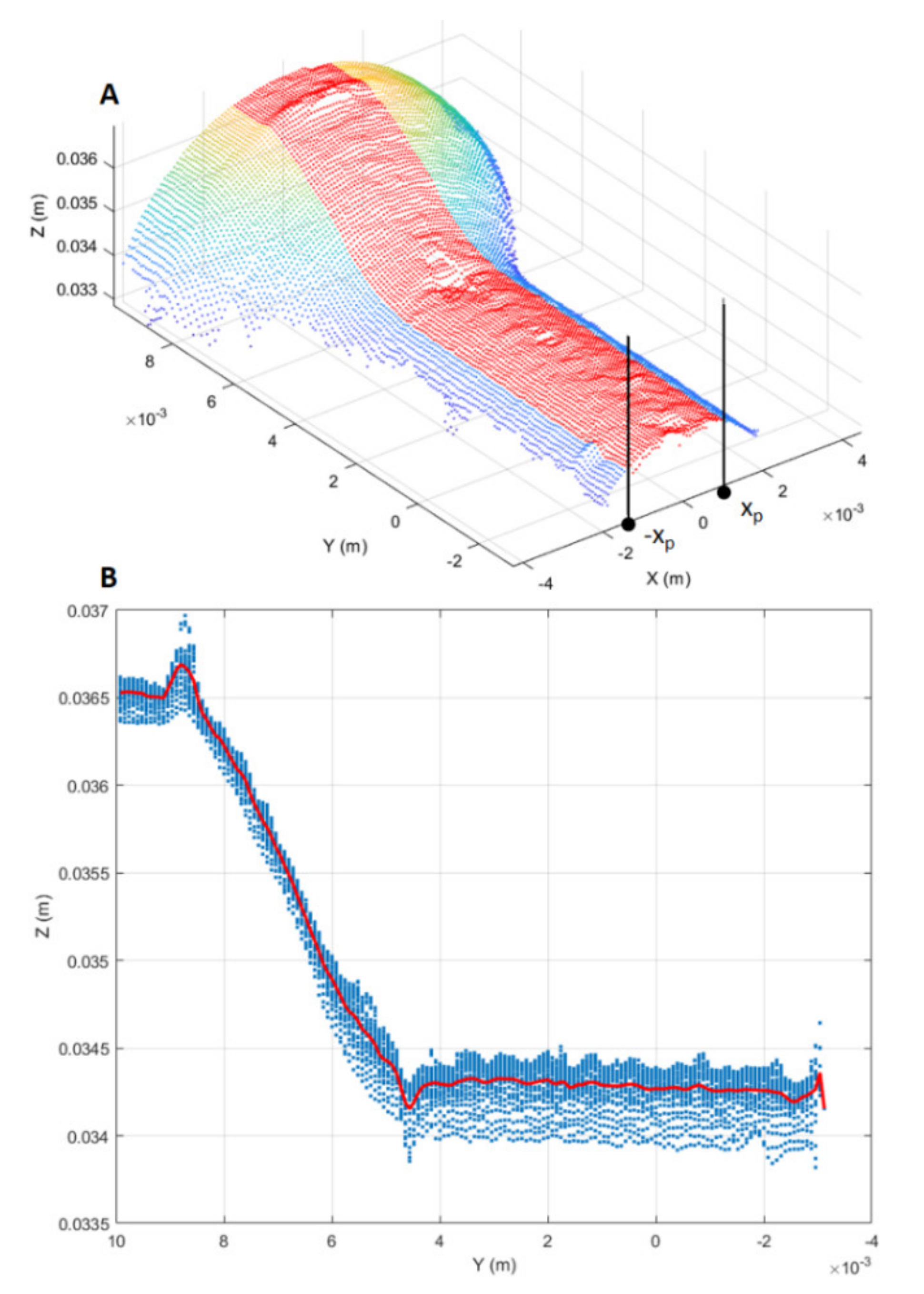
The RUL prediction based on the DNN was compared with that based on traditional ML methods (e.g., SVR). To do so, alongside the two-dimensional deformation representations mentioned above, one-dimensional representations were also considered, i.e., longitudinal profiles of the punch tool. The extraction process of longitudinal profiles, shown in Figure 9, consisted of three main steps. Firstly, a profile region was selected from the cropped point cloud by taking points such that (Figure 9A).
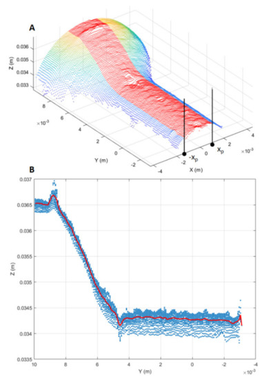
Figure 9.
Longitudinal profile extraction. (A) Longitudinal point-cloud region (red points) from which the longitudinal profile is estimated. (B) Estimated longitudinal profile (red curve) from the point cloud projection on the YZ plane.
Secondly, the selected point-cloud region was projected onto the YZ plane. Thirdly, the longitudinal profile was estimated averaging the projected region along the Z-axis direction (Figure 9B).
3.3. Evaluation Metrics
Three different evaluation metrics were adopted in this study, i.e., scoring function (SF), root mean square error (RMSE), and mean absolute percentage error (MAPE). The first two metrics were selected since they are commonly adopted in the literature on RUL prediction [32], while the third was considered as it allows for more subtle evaluations than the other two.
Given a total number of sampled machining cycles (i.e., 3D scans), let be the RUL at the machining cycle , the estimated version of , and the prediction error, the SF is defined as follows:
Furthermore, the RMSE is defined as follows:
Finally, MAPE is given by:
3.4. DNN Architectures
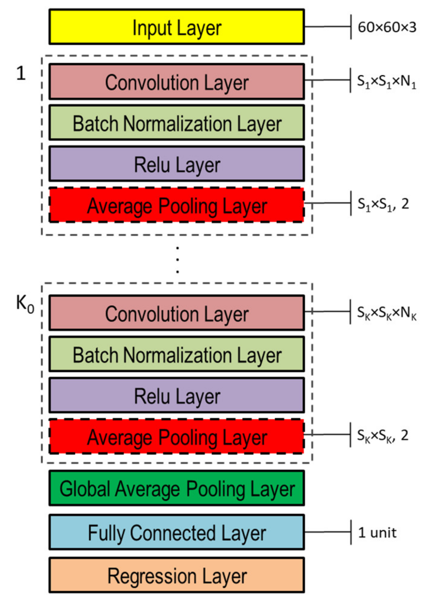
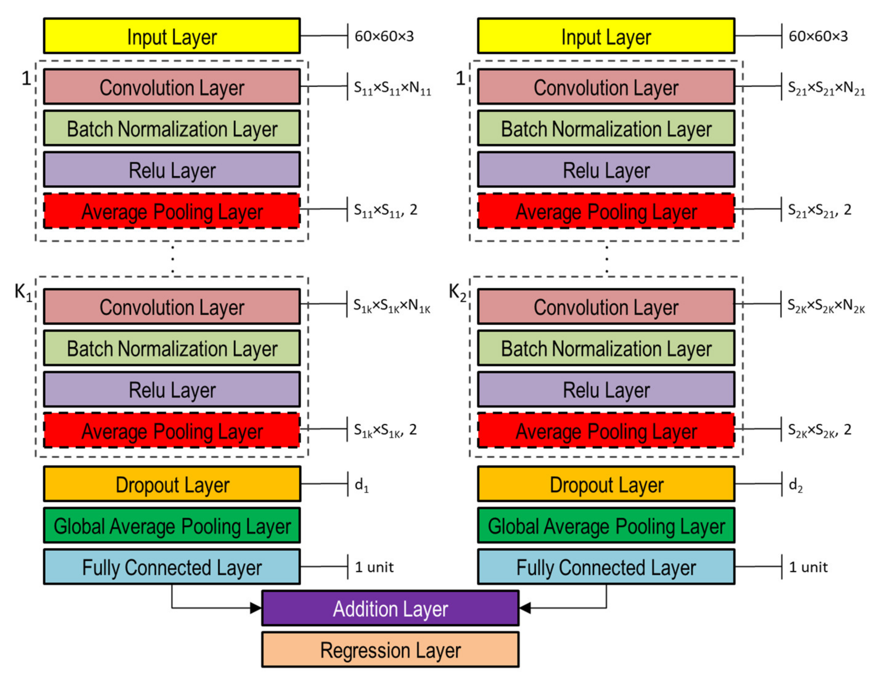
The DNNs used in this study to capture the representation information from preprocessed inputs, i.e., depth and normal maps provided as false-color images (Figure 8), were based on CNN [46]. Both single- and double-head DNNs were investigated, whose general architectures are shown in Figure 10 and Figure 11, respectively. Basically, they are composed of an input layer receiving depth or normal maps, resized to 60 × 60 pixels color (3-channels) images, followed by ( and in the double-head case) blocks including the following four layers: (1) convolution, (2) batch normalization, (3) rectified linear unit (ReLU), and (4) global average pooling.

Figure 10.
Single-head general architecture of CNN-based DNN for processing either depth or normal maps provided as color image inputs.
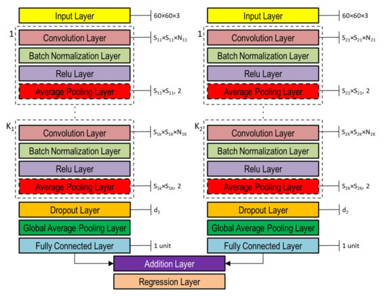
Figure 11.
Double-head general architecture of CNN-based DNN for processing both depth and normal maps provided as color image inputs.
CNN feature learning is based on the convolution operation implemented by applying a kernel to input images (i.e., local receptive field) whose response provides the so-called feature map. Let be an input image, W a kernel of size (a square kernel was considered in this study, but in general it may have a rectangular size) whose weights are adjusted in a feedforward way, the feature map computed at is given as follows:
where the summation is the convolution operation as the kernel slides over the image channel .
During the feedforward process, the output of a generic convolution layer at is given as follows:
where is the activation function used to introduce nonlinearity to feature maps, and is the bias term. In this study, the ReLU activation function was used which performs an element-wise threshold operation, i.e., sets to zero any input value less than zero:
The batch normalization layer, inserted between convolution and nonlinear activation (ReLU) layers, allows training to be sped up and the network to be regularized, reducing initialization sensitivity, i.e., it facilitates the convergence to good local minima without cumbersome initial parameter setting. Given an input element the batch normalization layer provides the following normalization:
where and are, respectively, mean and variance estimated over spatial, time and observation dimensions for each channel independently, whereas is a constant used to improve numerical stability if variance is too small.
The average pooling layer performs down-sampling by providing average values of its input as output and thus reducing the connection number to the next layer, which helps to mitigate overfitting. The pool size adopted in this study was the same as the corresponding convolution layer in each CNN block, whereas the stride (i.e., step size with which the pooling layer scans through the input) was fixed at 2. The effect of the dropout layer is to turn off (set to zero), with probability , a certain number of input elements randomly chosen. Such dropout operation has been shown to help prevent network overfitting [47]. In this study, the dropout layer was adopted only in the double-head case with and in the two heads, respectively (Figure 11).
The global average pooling layer provides further down-sampling by fully averaging the feature map. It is usually used before the final fully connected layer to reduce the size of activations, i.e., less weights, thus leading to a lower network size. The purpose of fully connected layers is to combine features to identify larger patterns. Thus, all the neurons in a fully connected layer are connected to all the neurons of the previous layer.
In case of classification problems, the last fully connected layer provides the features to perform classification, thus, its output size is equal to the number of classes being classified. In case of regression problems, the output size is equal to the number of regression variables, which is one in this study. In both single- and double-head architectures, the continuous RUL value was finally estimated in the regression layer by minimizing the loss (i.e., not-normalized half mean squared error), which in the case of this study with only one regression variable, reduces to .
Generally, the learning process is cast as an optimization problem of minimizing the loss function. In this study, the stochastic gradient descent (SGD) [48] was used as an optimization scheme. In SGD training, a mini-batch is stochastically selected at each time step, instead of using the entire training set, thus improving computing speed. Two relevant SGD parameters are initial learning rate and momentum . If is too low, the training process takes a long time, whereas if it is too high, the training might result in being suboptimal or divergent.
The momentum is a technique used in conjunction with SGD that adjusts the contribution of gradients at previous steps to determine the direction to proceed, instead of using only the gradient at the current step. If is equal to zero there is no contribution from previous steps, whereas if is one the contribution from previous steps is maximal. In this study, the network hyperparameters in the single-head case and were determined using a genetic optimization algorithm as discussed in the following subsection. Note that the average polling layer included in each CNN block is optional and its inclusion or exclusion was also considered among the network hyperparameters subject to optimization through binary array variables, as detailed in the following subsection.
In addition to the architectures shown in Figure 10 and Figure 11, pretrained networks were also evaluated. The adoption of pretrained models offers multiple advantages, such as the possibility to exploit complex models without having to train them from scratch, even when little training data are available (used to fine-tune the pretrained model) without running into overfitting problems, commonly found in the presence of small training data sets. The technique underlying pretrained models is called transfer learning [49] and, basically, allows the knowledge already learned from one domain to be applied to another.
However, the transfer of knowledge from one domain to another is not always feasible. When the source domain is not sufficiently related to the destination domain, or when the transfer methodology is not able to take advantage of relationships between domains, this can lead to negative transfer [49]. For that reason, in this study, the most popular state-of-the-art pretrained models reported in Table 1 were evaluated, and their prediction performance was compared with that of network architectures discussed above. Since such pretrained networks are designed for classification problems, they were adapted by substituting the last three layers, i.e., the global average pooling layer, the softmax layer, and the classification layer, with a fully connected layer with one output neuron followed by a regression layer.

Table 1.
Pretrained networks evaluated for transfer learning.
3.5. Genetic Optimization
The parameters of the network architectures shown in Figure 10 and Figure 11 were optimized by means of a genetic optimization technique. GAs are population-based optimization methodologies that take their cue from the evolutionary process of living beings, i.e., the metaphor of natural biological evolution [64]. GAs iteratively implement a series of operations to manipulate populations of candidate solutions (i.e., chromosomes) to produce new solutions by means of genetic functionals such as reproduction, crossover, and mutation. Ultimately, they are inspired by Darwin’s theory of evolution [65] and relative principles of reproduction, genetic recombination, and survival of the fittest. The population of chromosomes (i.e., candidate solutions) is evaluated through the attribution of a score carried out through a so-called fitness function, the formulation of which depends on the specific optimization problem.
In this study, the fitness function built network architectures and evaluated them, providing as output the MAPE value obtained from testing. Thus, the optimization problem was formulated as follows:
where are optimization variables, continuous or integer valued, bounded between and , respectively, defining candidate network architectures as better explained in the following. The number of optimization variables was for single-head architectures (Figure 10) and for double-head architectures (Figure 11). For both architectures, the number of CNN blocks ranged from four to six, i.e., .
In the single-head case, the optimization variables were , where represented the filter sizes, specified the number of filters, the presence or not of average pooling layers, the initial learning rate, and the momentum. In the double-head case, instead, the optimization variables were , and represented the filter sizes, number of filters, and presence or not of average pooling layers for the first head, whereas were the filter sizes, number of filters, and presence or not of average pooling layers for the second head. was the initial learning rate, the momentum, the dropout probability for the first head, and the dropout probability for the second head.
Regarding the convolutional filter sizes, i.e., (single-head) or and (double-head) variables, odd square dimensions ranging from 3 × 3 to 29 × 29 were evaluated by considering all possible combinations taking () at a time. For example, in the case of , corresponded to , to , to , etc., and to (23,25,27,29); after that, it continued in reverse order, i.e., corresponded to (29,27,25,23), corresponded to (29,27,25,21), and so on. Regarding the number of filters, i.e., (single-head) or and (double-head) variables, power of two between 8 and 256 were considered in incremental order. Thus, for example, in the case gave , gave , gave , and so on.
Since the average pooling layers, depicted in Figure 10 and Figure 11 with dashed lines, were optional, their presence or absence were regulated by variables (single-head) or and (double-head), representing the configurations of a binary array , where 1 in -th position (with ) indicated the presence of average pooling layer at the end of the -th CNN block. For example, in the case of , corresponded to , corresponded to , to , and so on. All previously discussed optimization variables are summarized in Table 2.
Table 2.
Lower and upper bounds of all optimization variables.
In this study, both suggested DNNs (Figure 10 and Figure 11) and pretrained ones (Table 1) were implemented and evaluated using the MathWorks® Deep Learning Toolbox (v 14.2, R2021a, MathWorks Inc., Natick, MA, USA) [66]; whereas, genetic optimization was performed using the MathWorks® Optimization Toolbox (v 9.1, R2021a, MathWorks Inc., Natick, MA, USA) [67].
3.6. SVR Based Estimation
As a further comparison, the previously presented DNN-based models were compared with more traditional ML methods such as SVR. Since the presence of irrelevant or redundant information could slow down or make prediction algorithms less accurate, it is necessary, before the learning model, to distinguish between relevant and unnecessary features. For this reason, the first step was to reduce the dimensionality of the profile data (Figure 9B) using the PCA approach [68].
The profile data were represented in YZ plane by curves , , with typically ranging between 156 to 164 depending on the specific point cloud considered. After the PCA application, the reduced profile data were given by , since the percentage of variance explained by the first two principal components was 100%. Ultimately, profile feature data used to train and test the SVR model was written as follows:
To achieve a good compromise between processing speed and accuracy, in this study, the epsilon-insensitive SVR (i.e., SVR) [69,70] was adopted, in which the epsilon parameter controls the amount of error allowed in the model. Given training data , the goal is to find a function that deviates from RUL values by an amount no greater than while at the same time being as flat as possible.
In the linear case, assuming that the training data set is composed of profiles and corresponding RUL values with , the linear function takes the form , where is the dot product, and such that is minimum to ensure flatness. The problem can be stated in term of convex optimization as follows:
Since a function satisfying these constraints for all points may not exist, in practice, slake variables are introduced, analogously to the concept of “soft margin” in SVM. With the addition of the slake variables problem (9) becomes [66]:
where the positive parameter controls the penalty imposed on observations that fall outside the margin, playing a regularizing role to prevent overfiting.
In the nonlinear case, the dot product is replaced with a kernel function which maps training data to a high-dimensional space. Some popular kernel functions evaluated in this study are reported in Table 3.
Table 3.
Kernel functions evaluated in this study.
4. Results
The performance results of the genetically optimized network architectures are provided in Table 4. In the single-head case, the convention used for the model name is a prefix “go” which stands for genetically optimized, followed by the number of CNN blocks and the suffix “normal” or “depth” depending on the type of map the model was tested on. Thus, for instance, the name of the model genetically optimized with four CNN blocks and tested on normal maps is “go4normal”. Instead, in the double-head architectures, since they were tested on both normal and depth maps, the naming convention consists of the suffix “go” followed by the number of blocks for the two heads, for example, “go4+4” indicates a model with four blocks for each head. In addition to the three metrics defined in (1), (2), and (3), the last column of Table 4 provides the time required to train each model.
Table 4.
RUL prediction performance obtained with genetically optimized networks tested on both depth and normal maps.
The population size was 50 in single-head architectures (5 optimization variables) and 200 in double-head ones (10 optimization variables), for a total number of 10,000 and 40,000 iterations, respectively. For each candidate architecture, the model was trained for 100 epochs, randomizing the validation data set to each epoch. To achieve the final performance, the results of the top 100 architectures based on the fitness function (i.e., the MEPA metric) were averaged.
The pretrained models (Table 1) tested on normal and depth maps are provided in Table 5 and Table 6, respectively. The last columns of these tables report the fine-tuning time (FTT), i.e., the time elapsed to fine-tune each pretrained model for 30 epochs. Also in this case, performance results were averaged by repeating training and testing 100 times for each model.
Table 5.
RUL prediction performance obtained with pretrained networks tested on normal maps.
Table 6.
RUL prediction performance obtained with pretrained networks tested on depth maps.
As regards the classical approaches based on SVR, three kernels, i.e., linear, Gaussian and polynomial of order 3, 4, 5, and 6, were tested. The performance results obtained with the approaches based on SVR are reported in Table 7. In this study, SVR was considered as a benchmark for evaluating the goodness of DNN-based models.
Table 7.
RUL prediction performance obtained with SVR algorithms tested on surface profiles.
A comprehensive overview of all achieved results is shown in Figure 12. As can be seen from this figure, the models that performed best are the genetically optimized ones (numbers from no. 1 to 15), while most of the pretrained models (from no. 16 to 51) performed worse than the SVR algorithms (from no. 52 to 57), with the exception of the pretrained models, googlenet (no. 17), vgg16 (no. 32), vgg19 (no. 33), on maps of normal vectors and the pretrained models, googlenet (no. 35), alexnet (no. 49), and vgg19 (no. 51), on depth maps.
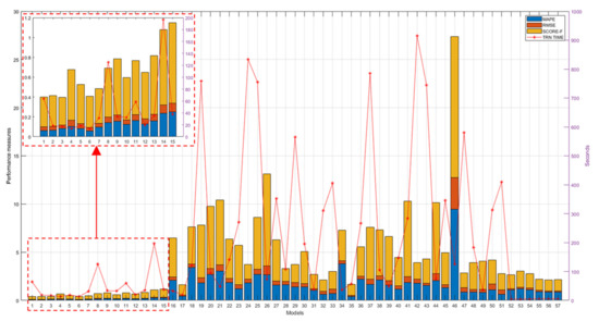
Figure 12.
Performance measures (left y-axis) and TTs/FTTs (right y-axis) of all evaluated models.
Figure 12 also reports training times (TTs) of genetically optimized and SVR-based models and FTTs of pretrained models, revealing on average longer times for the pretrained models (from no. 18 to 51), on average shorter times for the genetically optimized models (from no. 1 to 15), and very short times for the SVR models (from no. 52 to 57). Note that, to facilitate reading, the numbering reported on the x-axis in Figure 12 matches the model numbers reported in the first column of the tables from Table 1, Table 2, Table 3, Table 4, Table 5, Table 6, Table 7, Table 8 and Table 9, for a total of 57 examined models.
Table 8.
Network configuration of genetically optimized single-head DNN architectures.
Table 9.
Network configuration of genetically optimized double-head DNN architectures.
Finally, the network configurations of genetically optimized single- and double-head DNN architectures are reported in Table 8 and Table 9, respectively. The reported parameters refer to best-fit models resulting from the genetic optimization process. The last columns show the number of learned parameters (learnables) of each architecture. The genetic optimization process lasted an average of 53 h for each single-head architecture and approximately 632 h for each dual-head architecture. The total duration of the genetic optimization process was approximately 250 days on a computer system equipped with a graphics processing unit (GPU) and configured as follows: Intel® Core™ i7-5820K CPU @ 3.30 GHz, 16 GB DRAM, and NVIDIA GeForce GTX TITAN X GPU (Maxwell family) with 12 GB GRAM.
5. Discussion
The use of profilometric scanning sensors allows surface deformations to be appreciated with micrometric precision in the form of 3D point clouds. On the other hand, the organization of 3D point clouds into bidimensional image-like maps, as proposed in this study, enables us to make the most of the potential of CNN-based DNN architectures, originally designed to process image data. Furthermore, in the case of RUL depending on surface deformations, two-dimensional maps offer the advantage of representing the state of system (i.e., punch tool in this study) deterioration in a cumulative way. Therefore, under such conditions, the RUL can be reliably estimated from a single image, that is from a single depth or normal map.
Pretrained networks with transfer learning are advantageous since they allow small training data sets to be dealt with and the often-cumbersome process of generating problem-specific networks to be overcome. However, they are not always suitable, especially when data distributions are very dissimilar between source and target domains.
The definition of the most suitable DNN architecture for the problem under consideration, however, is not an easy task. In general, it involves identifying various configuration parameters (hyperparameters) through a trial-and-error process. The transfer learning method offers the indisputable advantage of simplifying this often cumbersome process of generating ad-hoc DNN architectures. In addition, pretrained models require the use of a small amount of training data for fine-tuning, allowing the additional problem of reduced amount of training data to be addressed [35].
Keeping in mind the aforementioned advantages, in this study, the transfer learning technique was evaluated in correspondence with the main pretrained models, as reported in Table 1, with both depth and normal maps. However, the performance results obtained were generally lower than the more traditional SVR approach taken as a reference (Figure 12). Only the pretrained models googlenet (MAPE equal to 0.452 with normal maps and 0.416 with depth maps), vgg16 (MAPE = 0.615 with normal maps), vgg19 (MAPE equal to 0.698 with normal maps and 0.648 with depth maps), and alexnet (MAPE = 0.822 with depth maps) performed slightly better than the SVR approach (MAPE = 0.857 with polynomial kernel of order 6), but requiring on average 35 times more time for fine-tuning than SVR requires for training.
In this study, the problem of defining ad-hoc (problem-specific) architectures was addressed by resorting to genetic optimization. In this way, a total amount of 15 architectures were optimized, of which 6 were single-headed (three for each type of map), shown in Table 8 and Table 9 double-headed, as shown in Table 9. The performance results reported in Figure 12 (see the magnification in the upper left corner) confirm the superiority of the genetically optimized architectures over the pretrained ones. The drop in performance found with the transfer learning method can be explained by the fact that feature distributions across the two domains, source and target, were very different from each other. The pretrained models (Table 1), in fact, were pretrained using mostly “natural” images, while the images proposed in this study were obtained by mapping 3D point clouds in order to represent depths and normal vectors to the punch tool surface, resulting in “artificial” images with false colors.
Among the genetically optimized architectures, the single-headed models performed better than double-headed ones, with a slight predominance of models trained and tested on depth maps over those evaluated with normal maps. These results indicate that the use of two-headed models is not beneficial, and it is probably explained by poor correlations between features extracted from the two different types of maps, depth and normal, in representing deformation-induced degradation.
The results achieved in this study are in line with the state of the art in the literature. In particular, regarding CNN-based studies with image datasets; one of the best results presented in the literature was reported by Wu et al. [34]. In their study, the authors reported an average MAPE of 0.0476, which, however, was obtained with a very large data set consisting of 8400 images, while the TT was between 1.8 and 32.6 h (the authors have not provided specifications of used computing system). On the other hand, in the case of small data sets, one of the best results reported in the literature is that of Marei et al. [35] who achieved an average RMSE of 0.1654 with the Resnet18 pretrained model on a data set of 327 images, requiring 3358.4 s for fine-tuning on an NVIDIA GPU with 8GB Ram. However, it should be kept in mind that images of deteriorating components or parts of them (i.e., real world images, often obtained under a microscope and by stopping the machining system) were used in those studies. Therefore, the adaptation (or transfer learning) of pre-existing (or pretrained) CNN models was feasible, considering the similarity of feature distributions between domains. In the case, instead, of data sets consisting of time-series sensor data, Mo et al. [39] reported an average RMSE of 11.28 with the NASA C-MAPSS data set. A comparison between the results achieved in this study and the best results reported in the related literature is provided in Table 10.
Table 10.
Comparison between related studies and this study.
The proposed system has been conceived to be versatile, working in a completely automatic way. There is no need to disassemble the punch tool or stop the punch machine to capture scans. The used 3D sensor, attached to the punching machine, scans at regular intervals of pressing stops. Furthermore, it is important to note that both depths, normal maps and longitudinal profiles, allow the punch tool RUL to be estimated in a single shot, i.e., a single profile or map accounts for all deformations that have occurred up to that moment. This allows the processing of long sequences of profiles or maps to be avoided, reducing computational load and network architecture complexity.
Although the optimization process takes a long time, it only needs to be performed once for the type of punch tool used. In this study, three different punch tools were tested, characterized by different deformation modes, using the same network architectures. An aspect that deserves further investigation concerns the verification of whether the proposed architectures are also valid for predicting the RUL of other systems than the studied punch tool, but whose degradation still depends on the work surface deformation.
6. Conclusions
In this study, a DNN-based RUL prediction framework for a punch tool, whose deterioration is due to surface deformation, was investigated. The RUL prediction is part of PHM maintenance strategies, in which the continuous monitoring of equipment health conditions allows the degradation state to be predicted, improving strategic maintenance decisions and thus avoiding late or too premature corrective actions. In the case of deformation-related degradations represented by DNVMs, the findings of this research show that the development of ad-hoc DNN models, driven by genetic optimization, provides better performance than pretrained models, indicating that the use of “transfer learning” is not always the best route.
The main results achieved are threefold, as indicated below. Firstly, the surface deformation of the punch tool was represented through the definition of DNVMs, obtained from point clouds of 3D scans. Secondly, the RUL prediction was estimated considering the main pretrained models, obtaining lower or slightly higher performance than SVR-based classic ML, due to the different distribution of features between the transfer learning domains. Thirdly, genetically optimized architectures based on a variable number of CNN blocks, both single- and double-headed, were generated, achieving superior performance to pretrained models and in line with the state of the art in the literature. Furthermore, the advantage of the proposed solution lies in its non-invasiveness and continuous operation. In fact, the monitoring is carried out by means of a 3D scan sensor placed outside the machinery, whose high degree of precision allows point clouds to be captured without stopping the punching process.
Ongoing and future research focuses on experimentation of DNVMs in combination with genetically optimized DNN architectures for the RUL prediction of other systems whose deterioration depends on surface deformations. More specifically, mechanical systems having geometry and material different from those of the punch tool will be the object of future investigations. This will allow verification of the degree of dependence of the DNN architecture on the characteristics of the mechanical system subject to degradation.
Author Contributions
Conceptualization, G.D. and A.L.; methodology, G.D.; software, G.D.; validation, G.D. and A.L.; writing—original draft preparation, G.D.; writing—review and editing, G.D.; visualization, G.D.; supervision, A.L.; project administration, A.L. and P.S.; funding acquisition, P.S. All authors have read and agreed to the published version of the manuscript.
Funding
This research was funded by the Italian Ministry of Education and University (MIUR) under the program PON R&I 2014–2020, research project REACT, grant number ARS01_01031.
Institutional Review Board Statement
Not applicable.
Informed Consent Statement
Not applicable.
Data Availability Statement
Not applicable.
Acknowledgments
The authors would like to thank colleagues of Masmec SpA for their support.
Conflicts of Interest
The authors declare no conflict of interest. The funders had no role in the design of the study; in the collection, analyses, or interpretation of data; in the writing of the manuscript, or in the decision to publish the results.
References
- Atamuradov, V.; Medjaher, K.; Dersin, P.; Lamoureux, B.; Zerhouni, N. Prognostics and Health Management for Maintenance Practitioners—Review, Implementation and Tools Evaluation. Int. J. Progn. Health Manag. 2017, 8. [Google Scholar] [CrossRef]
- Silvestri, L.; Forcina, A.; Introna, V.; Santolamazza, A.; Cesarotti, V. Maintenance transformation through Industry 4.0 technologies: A systematic literature review. Comput. Ind. 2020, 123, 103335. [Google Scholar] [CrossRef]
- Kuo, C.-J.; Chien, C.-F.; Chen, J.-D. Manufacturing Intelligence to Exploit the Value of Production and Tool Data to Reduce Cycle Time. IEEE Trans. Autom. Sci. Eng. 2010, 8, 103–111. [Google Scholar] [CrossRef]
- Chien, C.-F.; Chen, C.-C. Data-Driven Framework for Tool Health Monitoring and Maintenance Strategy for Smart Manufacturing. IEEE Trans. Semicond. Manuf. 2020, 33, 644–652. [Google Scholar] [CrossRef]
- Si, X.-S.; Wang, W.; Hu, C.-H.; Zhou, D.-H. Remaining useful life estimation—A review on the statistical data driven approaches. Eur. J. Oper. Res. 2011, 213, 1–14. [Google Scholar] [CrossRef]
- Liao, L.; Köttig, F. A hybrid framework combining data-driven and model-based methods for system remaining useful life prediction. Appl. Soft Comput. 2016, 44, 191–199. [Google Scholar] [CrossRef]
- Wang, Y.; Zhao, Y.; Addepalli, S.N.P. Remaining Useful Life Prediction using Deep Learning Approaches: A Review. Procedia Manuf. 2020, 49, 81–88. [Google Scholar] [CrossRef]
- Elattar, H.M.; Elminir, H.K.; Riad, A.M. Prognostics: A literature review. Complex Intell. Syst. 2016, 2, 125–154. [Google Scholar] [CrossRef] [Green Version]
- Tran, V.T.; Pham, H.T.; Yang, B.-S.; Nguyen, T.T. Machine performance degradation assessment and remaining useful life prediction using proportional hazard model and support vector machine. Mech. Syst. Signal Process. 2012, 32, 320–330. [Google Scholar] [CrossRef] [Green Version]
- Bengio, Y.; Courville, A.; Vincent, P. Representation Learning: A Review and New Perspectives. IEEE Trans. Pattern Anal. Mach. Intell. 2013, 35, 1798–1828. [Google Scholar] [CrossRef]
- Zhao, R.; Yan, R.; Chen, Z.; Mao, K.; Wang, P.; Gao, R.X. Deep learning and its applications to machine health monitoring. Mech. Syst. Signal Process. 2019, 115, 213–237. [Google Scholar] [CrossRef]
- Shrestha, A.; Mahmood, A. Review of Deep Learning Algorithms and Architectures. IEEE Access 2019, 7, 53040–53065. [Google Scholar] [CrossRef]
- Pearson, K. On lines and planes of closest fit to systems of points in space. Philos. Mag. Ser. 1901, 2, 559–57223. [Google Scholar] [CrossRef] [Green Version]
- Hotelling, H. Analysis of a complex of statistical vari-ables into principal components. J. Educ. Psychol. 1933, 24, 417–441. [Google Scholar] [CrossRef]
- Fisher, R.A. The Use of Multiple Measurements in Taxonomic Problems. Ann. Eugen. 1936, 7, 179–188. [Google Scholar] [CrossRef]
- Hinton, G.E.; Salakhutdinov, R.R. Reducing the dimensionality of data with neural networks. Science 2006, 313, 504–507. [Google Scholar] [CrossRef] [PubMed] [Green Version]
- Ma, J.; Su, H.; Zhao, W.-L.; Liu, B. Predicting the Remaining Useful Life of an Aircraft Engine Using a Stacked Sparse Autoencoder with Multilayer Self-Learning. Complexity 2018, 2018. [Google Scholar] [CrossRef] [Green Version]
- Sun, C.; Ma, M.; Zhao, Z.; Tian, S.; Yan, R.; Chen, X. Deep transfer learning based on sparse autoencoder for re-maining useful life prediction of tool in manufacturing. IEEE Trans. Ind. Inform. 2018, 15, 2416–2425. [Google Scholar] [CrossRef]
- Ren, L.; Sun, Y.; Cui, J.; Zhang, L. Bearing remaining useful life prediction based on deep autoencoder and deep neural networks. J. Manuf. Syst. 2018, 48, 71–77. [Google Scholar] [CrossRef]
- Liao, L.; Jin, W.; Pavel, R. Enhanced Restricted Boltzmann Machine With Prognosability Regularization for Prognostics and Health Assessment. IEEE Trans. Ind. Electron. 2016, 63, 7076–7083. [Google Scholar] [CrossRef]
- Haris, M.; Hasan, M.N.; Qin, S. Early and robust remaining useful life prediction of supercapacitors using BOHB optimized Deep Belief Network. Appl. Energy 2021, 286, 116541. [Google Scholar] [CrossRef]
- Jiao, R.; Peng, K.; Dong, J.; Zhang, C. Fault monitoring and remaining useful life prediction framework for multiple fault modes in prognostics. Reliab. Eng. Syst. Saf. 2020, 203, 107028. [Google Scholar] [CrossRef]
- Ma, M.; Sun, C.; Chen, X. Discriminative deep belief networks with ant colony optimization for health status as-sessment of machine. IEEE Trans. Instrum. Meas. 2017, 66, 3115–3125. [Google Scholar] [CrossRef]
- Zhang, C.; Lim, P.; Qin, A.K.; Tan, K.C. Multiobjective Deep Belief Networks Ensemble for Remaining Useful Life Estimation in Prognostics. IEEE Trans. Neural Netw. Learn. Syst. 2016, 28, 2306–2318. [Google Scholar] [CrossRef] [PubMed]
- Frederick, D.K.; DeCastro, J.A.; Litt, J.S. User’s Guide for the Commercial Modular Aero-Propulsion System Simulation (C-MAPSS. 2007. Available online: https://core.ac.uk/download/pdf/10566552.pdf (accessed on 27 July 2021).
- LeCun, Y.; Bottou, L.; Bengio, Y.; Haffner, P. Gradient-based learning applied to document recognition. Proc. IEEE 1998, 86, 2278–2324. [Google Scholar] [CrossRef] [Green Version]
- Dhillon, A.; Verma, G.K. Convolutional neural network: A review of models, methodologies and applications to object detection. Prog. Artif. Intell. 2020, 9, 85–112. [Google Scholar] [CrossRef]
- Babu, G.S.; Zhao, P.; Li, X.-L. Deep Convolutional Neural Network Based Regression Approach for Estimation of Remaining Useful Life. In International Conference on Database Systems for Advanced Applications; Springer: Berlin/Heidelberg, Germany, 2016; pp. 214–228. [Google Scholar]
- Nectoux, P.; Gouriveau, R.; Medjaher, K.; Ramasso, E.; Chebel-Morello, B.; Zerhouni, N.; Varnier, C. PRONOSTIA: An experimental platform for bearings accelerated degradation tests. In Proceedings of the IEEE International Conference on Prognostics and Health Management, Denver, CO, USA, 18–21 June 2012; pp. 1–8. [Google Scholar]
- Heimes, F.O. Recurrent neural networks for remaining useful life estimation. In Proceedings of the 2008 International Conference on Prognostics and Health Management, Denver, CO, USA, 6–9 October 2008; pp. 1–6. [Google Scholar]
- Zheng, S.; Ristovski, K.; Farahat, A.; Gupta, C. Long Short-Term Memory Network for Remaining Useful Life estimation. In Proceedings of the 2017 IEEE International Conference on Prognostics and Health Management (ICPHM), Piscataway, NJ, USA, 19–21 June 2017; pp. 88–95. [Google Scholar]
- Li, X.; Ding, Q.; Sun, J.-Q. Remaining useful life estimation in prognostics using deep convolution neural networks. Reliab. Eng. Syst. Saf. 2018, 172, 1–11. [Google Scholar] [CrossRef] [Green Version]
- Malhotra, P.; TV, V.; Ramakrishnan, A.; Anand, G.; Vig, L.; Agarwal, P.; Shroff, G. Multi-sensor prognostics using an unsupervised health index based on LSTM encoder-decoder. arXiv 2016, arXiv:1608.06154. [Google Scholar]
- Wu, X.; Liu, Y.; Zhou, X.; Mou, A. Automatic Identification of Tool Wear Based on Convolutional Neural Network in Face Milling Process. Sensors 2019, 19, 3817. [Google Scholar] [CrossRef] [PubMed] [Green Version]
- Marei, M.; El Zaatari, S.; Li, W. Transfer learning enabled convolutional neural networks for estimating health state of cutting tools. Robot. Comput. Manuf. 2021, 71, 102145. [Google Scholar] [CrossRef]
- Deng, J.; Dong, W.; Socher, R.; Li, L.J.; Li, K.; Li, F.F. Imagenet: A Large-Scale Hierarchical Image Database. In Proceedings of the 2009 IEEE Conference on Computer Vision and Pattern Recognition, Miami, FL, USA, 20–25 June 2009; pp. 248–255. [Google Scholar]
- Russakovsky, O.; Deng, J.; Su, H.; Krause, J.; Satheesh, S.; Ma, S.; Fei-Fei, L. Imagenet large scale visual recognition challenge. Int. J. Comput. Vis. 2015, 115, 211–252. [Google Scholar] [CrossRef] [Green Version]
- Krizhevsky, A.; Nair, V.; Hinton, G. Cifar-10 and Cifar-100 Datasets. 2009. Available online: https://www.cs.toronto.edu/~kriz/cifar.html (accessed on 30 June 2021).
- Mo, H.; Custode, L.L.; Iacca, G. Evolutionary neural architecture search for remaining useful life prediction. Appl. Soft Comput. 2021, 108, 107474. [Google Scholar] [CrossRef]
- Li, X.; Jia, X.; Wang, Y.; Yang, S.; Zhao, H.; Lee, J. Industrial Remaining Useful Life Prediction by Partial Observation Using Deep Learning with Supervised Attention. IEEE/ASME Trans. Mechatron. 2020, 25, 2241–2251. [Google Scholar] [CrossRef]
- LMI Technologies. Gocator 3210 Datasheet—Large Field of View 3D Snapshot Sensor. Available online: https://lmi3d.com/resource/gocator-3210-datasheet-large-field-view-3d-snapshot-sensor/ (accessed on 14 July 2021).
- Besl, P.J.; McKay, N.D. A method for registration of 3-D shapes. IEEE Trans. Pattern Anal. Mach. Intell. 1992, 14, 239–256. [Google Scholar] [CrossRef]
- Chen, Y.; Medioni, G. Object modelling by registration of multiple range images. Image Vis. Comput. 1992, 10, 145–155. [Google Scholar] [CrossRef]
- Rousseeuw, P.J.; Leroy, A.M. Robust Regression and Outlier Detection; John Wiley & Sons: Hoboken, NJ, USA, 1987; Volume 589. [Google Scholar]
- Hoppe, H.; Derose, T.; Duchamp, T.; McDonald, J.; Stuetzle, W. Surface reconstruction from unorganized points. ACM SIGGRAPH Comput. Graph. 1992, 26, 71–78. [Google Scholar] [CrossRef]
- LeCun, Y.; Bengio, Y. Convolutional networks for images, speech, and time series. In The Handbook of Brain Theory and Neural Networks; MIT Press: Cambridge, MA, USA, 1995; p. 3361. [Google Scholar]
- Srivastava, N.; Hinton, G.; Krizhevsky, A.; Sutskever, I.; Salakhutdinov, R. Dropout: A Simple Way to Prevent Neural Networks from Overfitting. J. Mach. Learn. Res. 2014, 15, 1929–1958. [Google Scholar]
- Zinkevich, M.; Weimer, M.; Smola, A.J.; Li, L. Parallelized stochastic gradient descent. NIPS 2010, 4, 4. [Google Scholar]
- Ribani, R.; Marengoni, M. A Survey of Transfer Learning for Convolutional Neural Networks. In Proceedings of the 2019 32nd IEEE Conference on Graphics, Patterns and Images Tutorials (SIBGRAPI-T), Rio de Janeiro, Brazil, 28–31 October 2019; pp. 47–57. [Google Scholar]
- Iandola, F.N.; Han, S.; Moskewicz, M.W.; Ashraf, K.; Dally, W.J.; Keutzer, K. SqueezeNet: AlexNet-level accuracy with 50× fewer parameters and <0.5 MB model size. arXiv 2016, arXiv:1602.07360. [Google Scholar]
- Szegedy, C.; Liu, W.; Jia, Y.; Sermanet, P.; Reed, S.; Anguelov, D.; Erhan, D.; Vanhoucke, V.; Rabinovich, A. Going Deeper with Convolutions. arXiv 2014, arXiv:1409.4842. [Google Scholar]
- Szegedy, C.; Vanhoucke, V.; Ioe, S.; Shlens, J.; Wojna, Z. Rethinking the Inception Architecture for Computer Vision. In Pro-ceedings of the IEEE Conference on Computer Vision and Pattern Recognition. Las Vegas, NV, USA, 27–30 June 2016; pp. 2818–2826. [Google Scholar]
- Huang, G.; Liu, Z.; Van Der Maaten, L.; Weinberger, K.Q. Densely Connected Convolutional Networks. In Proceedings of the IEEE Conference on Computer Vision and Pattern Recognition 2017, Honolulu, HI, USA, 21–21 July 2017; pp. 4700–4708. [Google Scholar]
- Sandler, M.; Howard, A.; Zhu, M.; Zhmoginov, A.; Chen, L.C. Mobilenetv2: Inverted residuals and linear bottle-necks. In Proceedings of the IEEE Conference on Computer Vision and Pattern Recognition, Salt Lake City, UT, USA, 18–23 June 2018; pp. 4510–4520. [Google Scholar]
- He, K.M.; Zhang, X.Y.; Ren, S.Q.; Sun, J. Deep Residual Learning for Image Recognition. In Proceedings of the IEEE Conference on Computer Vision and Pattern Recognition, Las Vegas, NV, USA, 27–30 June 2016; pp. 770–778. [Google Scholar]
- Chollet, F. Xception: Deep Learning with Depthwise Separable Convolutions. In Proceedings of the IEEE Conference on Computer Vision and Pattern Recognition (CVPR), Honolulu, HI, USA, 21–26 July 2017; IEEE: New York, NY, USA, 2017; pp. 1251–1258. [Google Scholar]
- Szegedy, C.; Ioffe, S.; Vanhoucke, V.; Alemi, A.A. Inception-v4, inception-resnet and the impact of residual connections on learning. In Proceedings of the 31st AAAI Conference on Artificial Intelligence, San Francisco, CA, USA, 4–9 February 2017. [Google Scholar]
- Zhang, X.; Zhou, X.; Lin, M.; Sun, J. ShuffleNet: An Extremely Efficient Convolutional Neural Network for Mobile Devices. In Proceedings of the 2018 IEEE/CVF Conference on Computer Vision and Pattern Recognition, Salt Lake City, UT, USA, 18–23 June 2018; pp. 6848–6856. [Google Scholar]
- Zoph, B.; Vasudevan, V.; Shlens, J.; Le, Q.V. Learning Transferable Architectures for Scalable Image Recognition. In Proceedings of the 2018 IEEE/CVF Conference on Computer Vision and Pattern Recognition, Salt Lake City, UT, USA, 18–23 June 2018; pp. 8697–8710. [Google Scholar]
- Redmon, J. Darknet: Open-Source Neural Networks in c. 2013. Available online: https://pjreddie.com/darknet/ (accessed on 23 July 2021).
- Tan, M.; Le, Q. EfficientNet: Rethinking Model Scaling for Convolutional Neural Networks. In Proceedings of the International Conference on Machine Learning, Long Beach, CA, USA, 9–15 June 2019; pp. 6105–6114. [Google Scholar]
- Krizhevsky, A.; Sutskever, I.; Hinton, G.E. ImageNet classification with deep convolutional neural networks. Adv. Neural Inf. Process. 2012, 25, 1097–1105. [Google Scholar] [CrossRef]
- Simonyan, K.; Zisserman, A. Very deep convolutional networks for large-scale image recognition. arXiv 2014, arXiv:1409.1556. [Google Scholar]
- Mitchell, M. An Introduction to Genetic Algorithms; MIT Press: Cambridge, MA, USA, 1998. [Google Scholar]
- Darwin, C. On the Origin of Species by Means of Natural Selection; J. Murray: London, UK, 1859. [Google Scholar]
- Beale, M.; Hagan, M.; Demuth, H. Deep Learning Toolbox™ Reference. MATLAB (r) R2021a. The MathWorks, Inc. 2021. Available online: https://it.mathworks.com/help/pdf_doc/deeplearning/nnet_ref.pdf (accessed on 27 July 2021).
- Optimization Toolbox™ User’s Guide. MATLAB (r) R2021a. The MathWorks, Inc. Available online: https://it.mathworks.com/help/pdf_doc/optim/optim.pdf (accessed on 27 July 2021).
- Cao, L.; Chua, K.; Chong, W.; Lee, H.; Gu, Q. A comparison of PCA, KPCA and ICA for dimensionality reduction in support vector machine. Neurocomputing 2003, 55, 321–336. [Google Scholar] [CrossRef]
- Sain, S.R.; Vapnik, V.N. The Nature of Statistical Learning Theory. Technometrics 1996, 38, 409. [Google Scholar] [CrossRef]
- Smola, A.J.; Schölkopf, B. A tutorial on support vector regression. Stat. Comput. 2004, 14, 199–222. [Google Scholar] [CrossRef] [Green Version]


Publisher’s Note: MDPI stays neutral with regard to jurisdictional claims in published maps and institutional affiliations. |
© 2021 by the authors. Licensee MDPI, Basel, Switzerland. This article is an open access article distributed under the terms and conditions of the Creative Commons Attribution (CC BY) license (https://creativecommons.org/licenses/by/4.0/).