
Gaze Focalization System for Driving Applications Using OpenFace 2.0 Toolkit with NARMAX Algorithm in Accidental Scenarios

 , ,
, ,  , ,
, ,  ,
, 
Abstract
:1. Introduction
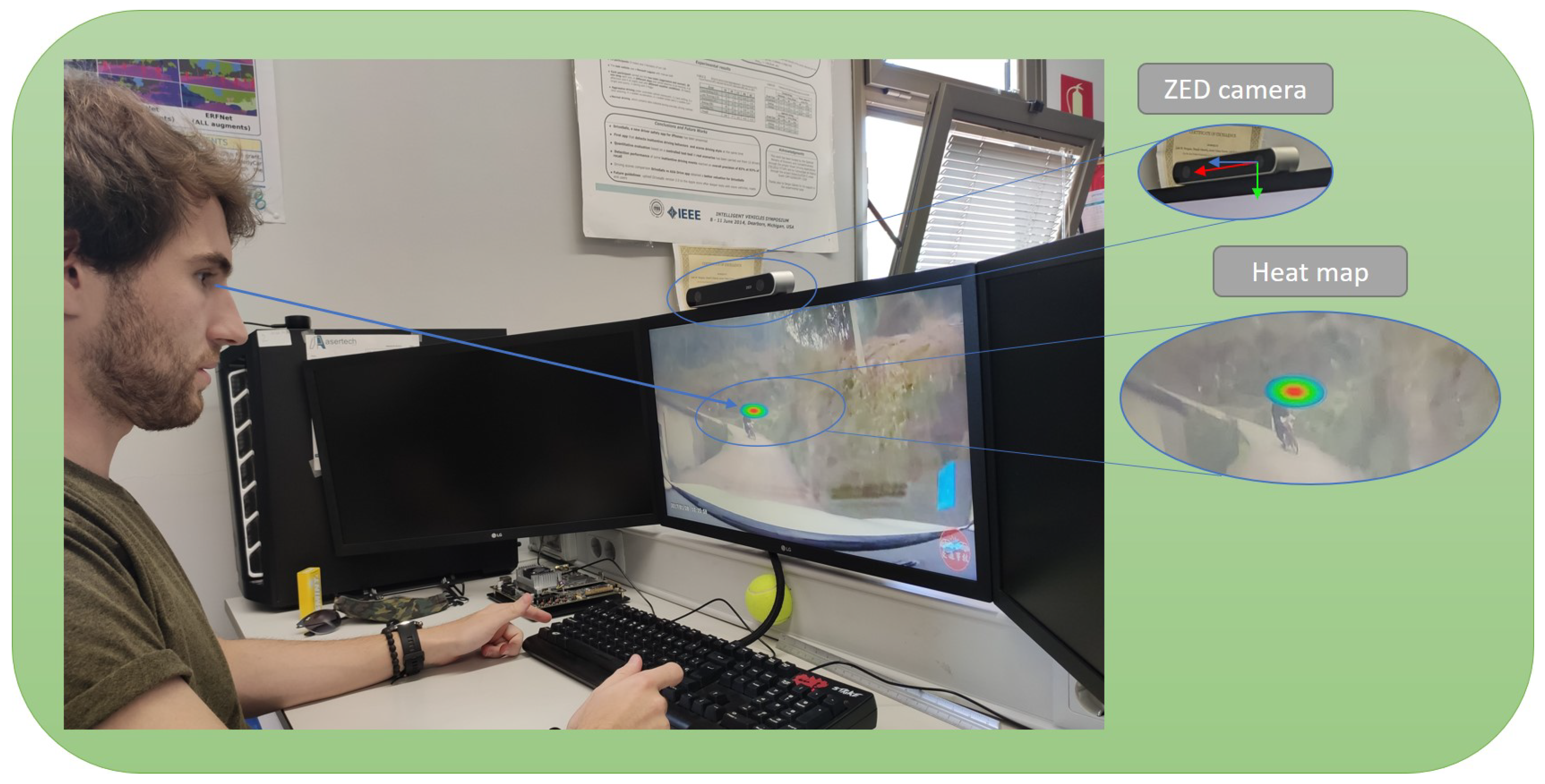
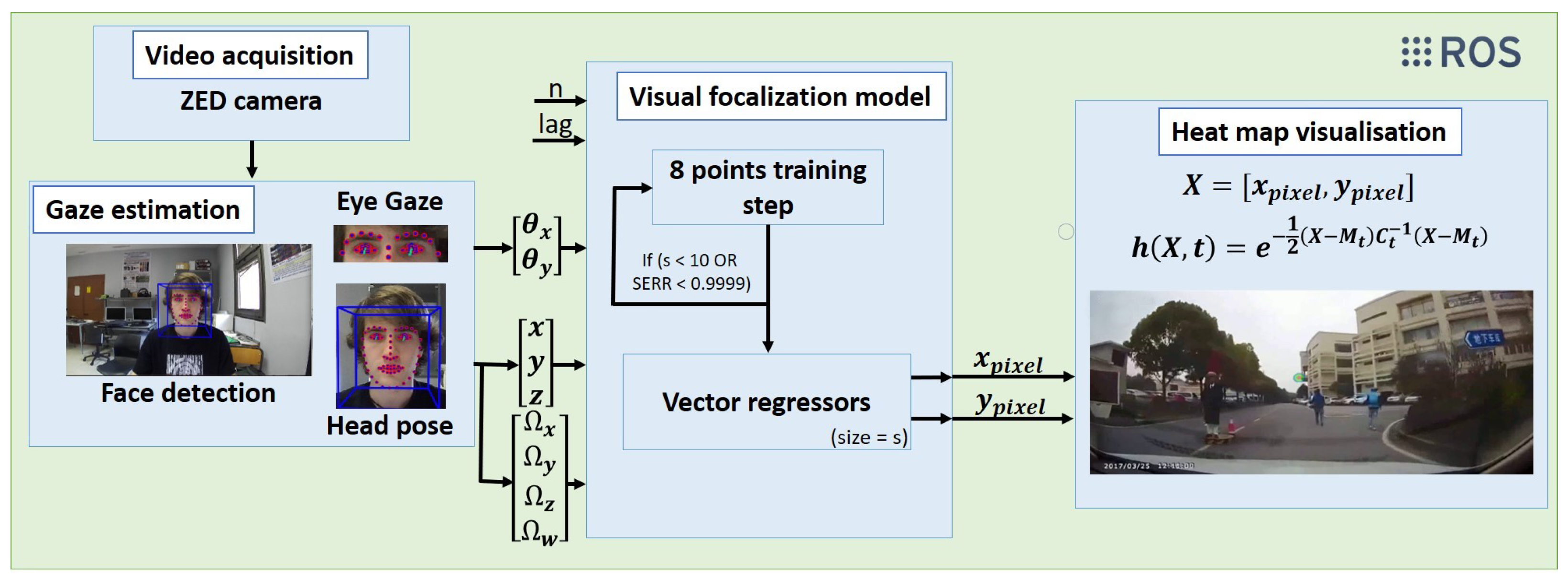
2. System Architecture
2.1. Video Acquisition
2.2. Gaze Estimation
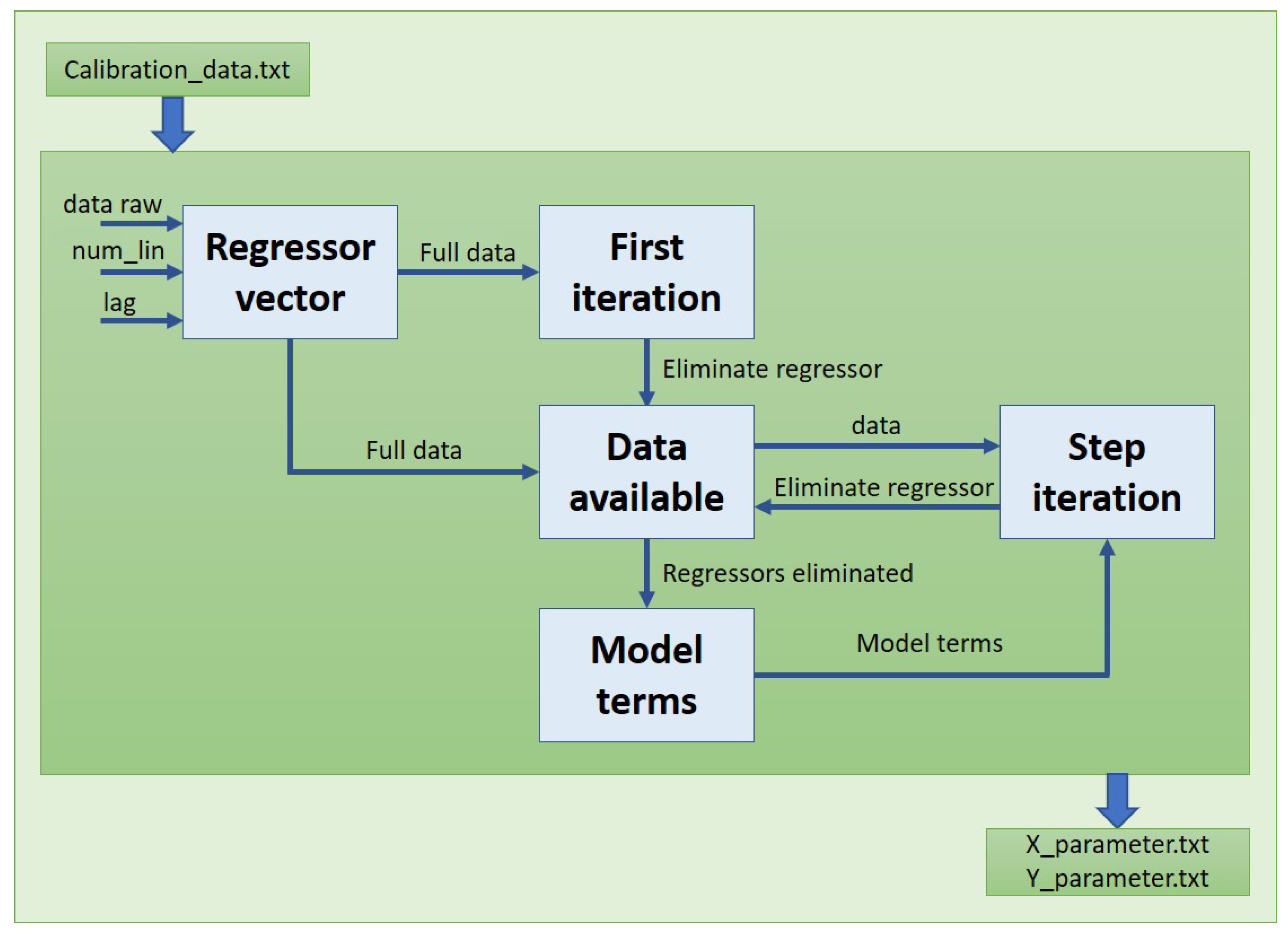
2.3. Visual Focalization Model
- Past signal terms (AR);
- Past noise terms (MA);
- Other signal with a possible delay (X).
- Structure detection—“What parts are in the model?”;
- Parameter estimation—“What are the values of the model coefficients?”;
- Model validation—“Is the model correct and unencumbered?”;
- Prediction—“What does the modeled signal look like in the future?”.
- Polynomial degree;
- Term degree;
- Logarithm;
- Neuronal network;
- Superposition of the above methods.
2.3.1. OLS
2.3.2. ERR
2.3.3. FROLS
Step 1. Data Collection
Step 2. Defining the Modelling Framework
- What is the maximum delay of the AR term ()? (Output signal)?
- What is the maximum delay of external signals ()? (Input signal)?
- What nonlinearities are predicted and what is their maximum degree (l)?
Step 3. Determination of the Regressor Vector
Step 4. Choosing the First Element
Step 5. Selecting the Next Elements of the Model
2.3.4. Modelling Process Analysis
2.3.5. Determination of the Final Model
- Gaze angle X ();
- Gaze angle Y ();
- Head position X (x);
- Head position Y (y);
- Head position Z (z);
- Head rotation X ();
- Head rotation Y ();
- Head rotation Z ();
- Head rotation W ().
2.4. Heat Map Visualisation
3. Experimental Results
3.1. Visual Focalization Model Evaluation
3.2. Camera Parameters
3.3. Camera Position
3.4. Glasses
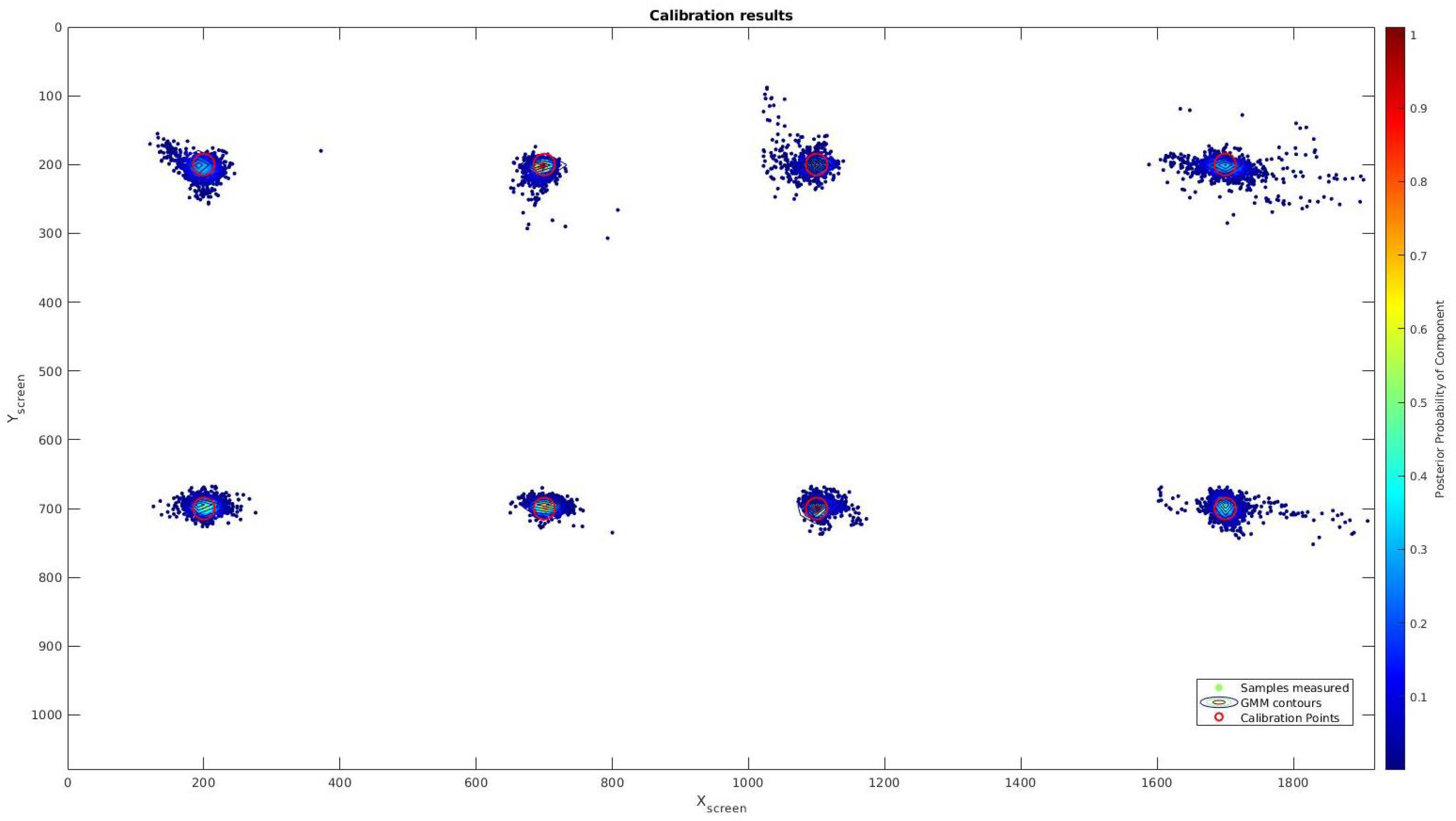
3.5. Precision Test
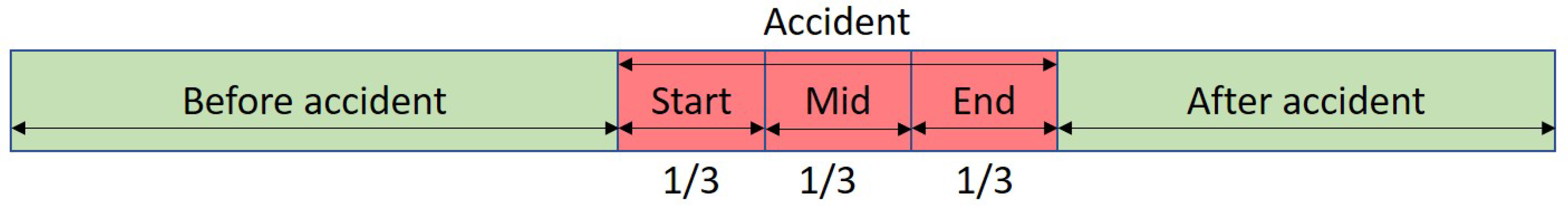
3.6. DADA2000 Evaluation
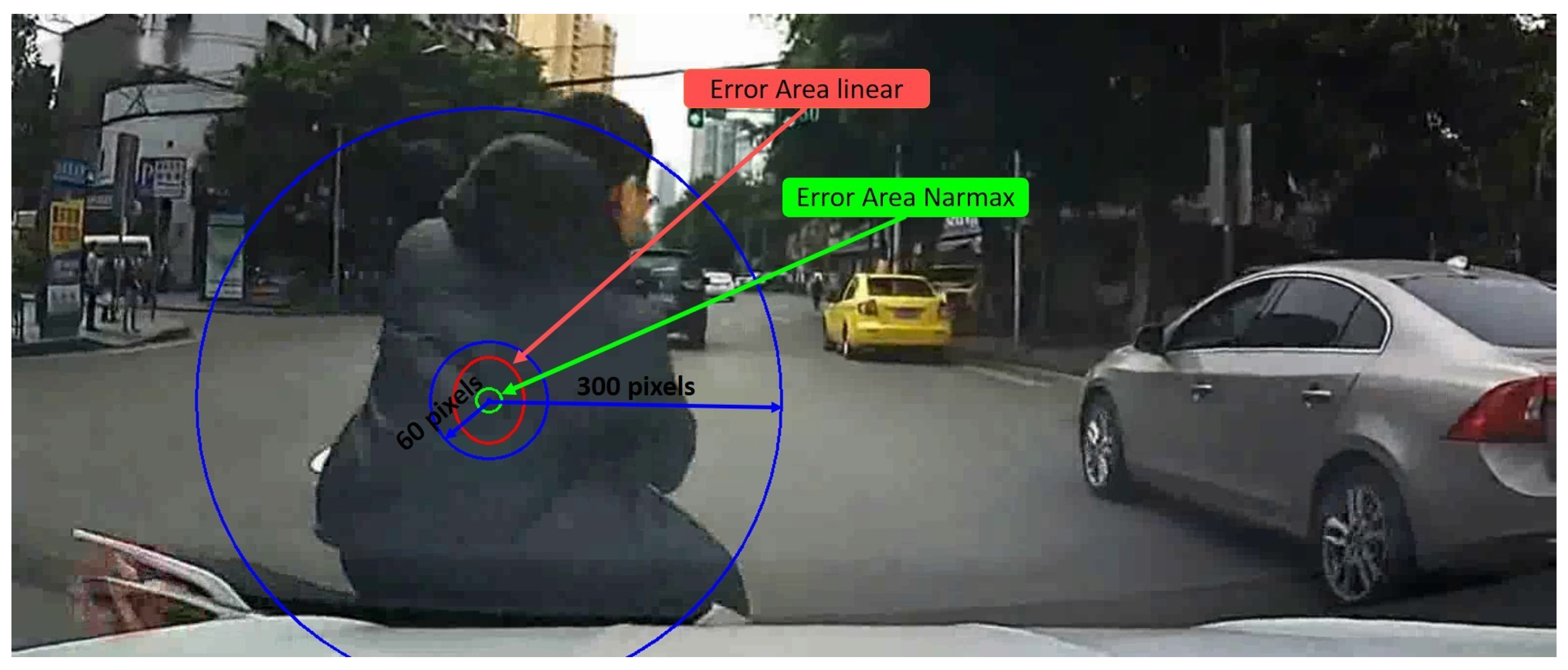
3.6.1. Crash Object Detection in DADA2000 Benchmark
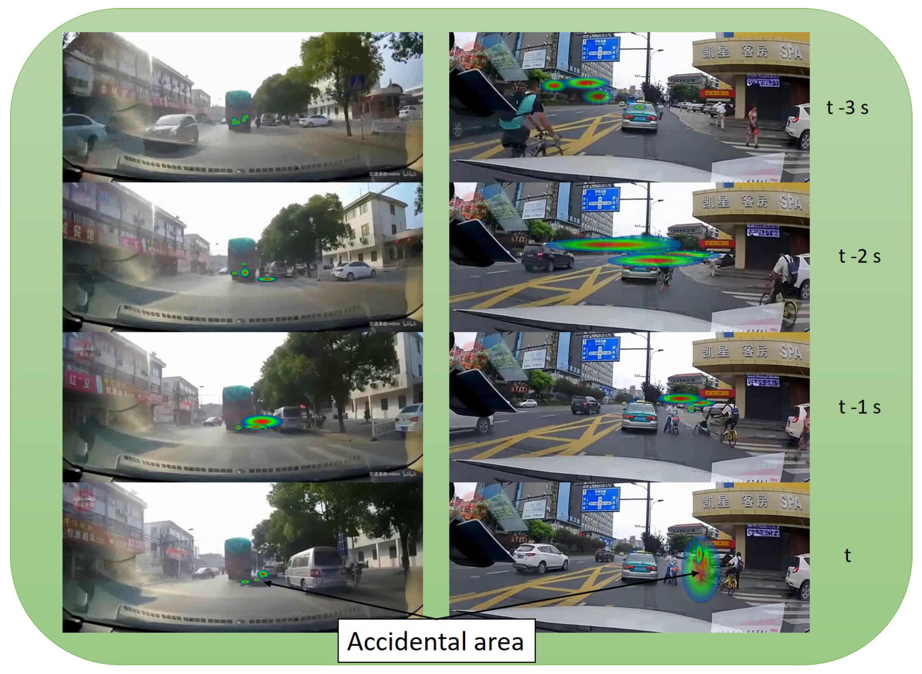
3.6.2. Heat Focalization Map on DADA2000
4. Conclusions and Future Works
Author Contributions
Funding
Informed Consent Statement
Data Availability Statement
Acknowledgments
Conflicts of Interest
References
- Baltrusaitis, T.; Zadeh, A.; Lim, Y.C.; Morency, L.P. Openface 2.0: Facial behavior analysis toolkit. In Proceedings of the 2018 13th IEEE International Conference on Automatic Face & Gesture Recognition (FG 2018), Xi’an, China, 15–19 May 2018; pp. 59–66. [Google Scholar]
- Araluce, J.; Bergasa, L.M.; Gómez-Huélamo, C.; Barea, R.; López-Guillén, E.; Arango, F.; Pérez-Gil, Ó. Integrating OpenFace 2.0 Toolkit for Driver Attention Estimation in Challenging Accidental Scenarios. In Workshop of Physical Agents; Springer: Cham, Switzerland, 2020; pp. 274–288. [Google Scholar]
- Fang, J.; Yan, D.; Qiao, J.; Xue, J.; Wang, H.; Li, S. DADA-2000: Can Driving Accident be Predicted by Driver Attentionƒ Analyzed by A Benchmark. In Proceedings of the 2019 IEEE Intelligent Transportation Systems Conference (ITSC), Auckland, NZ, USA, 27–30 October 2019; pp. 4303–4309. [Google Scholar]
- SAE On-Road Automated Vehicle Standards Committee. Taxonomy and Definitions for Terms Related to On-Road Motor Vehicle Automated Driving Systems J3016_201401. SAE Stand. J. 2014, 3016, 1–16. [Google Scholar]
- Jimenez, F. Intelligent Vehicles: Enabling Technologies and Future Developments; Butterworth-Heinemann: Oxford, UK, 2017. [Google Scholar]
- Yang, L.; Dong, K.; Dmitruk, A.J.; Brighton, J.; Zhao, Y. A Dual-Cameras-Based Driver Gaze Mapping System With an Application on Non-Driving Activities Monitoring. IEEE Trans. Intell. Transp. Syst. 2019, 21, 4318–4327. [Google Scholar] [CrossRef] [Green Version]
- Dalmaijer, E.; Mathôt, S.; Stigchel, S. PyGaze: An open-source, cross-platform toolbox for minimal-effort programming of eyetracking experiments. Behav. Res. Methods 2013, 46. [Google Scholar] [CrossRef] [PubMed]
- Cognolato, M.; Atzori, M.; Müller, H. Head-mounted eye gaze tracking devices: An overview of modern devices and recent advances. J. Rehabil. Assist. Technol. Eng. 2018, 5, 2055668318773991. [Google Scholar] [CrossRef] [PubMed]
- Shen, J.; Zafeiriou, S.; Chrysos, G.G.; Kossaifi, J.; Tzimiropoulos, G.; Pantic, M. The First Facial Landmark Tracking in-the-Wild Challenge: Benchmark and Results. In Proceedings of the 2015 IEEE International Conference on Computer Vision Workshop (ICCVW), Santiago, Chile, 7–13 December 2015; pp. 1003–1011. [Google Scholar] [CrossRef] [Green Version]
- Xia, Y.; Zhang, D.; Kim, J.; Nakayama, K.; Zipser, K.; Whitney, D. Predicting driver attention in critical situations. In Asian Conference on Computer Vision; Springer: Cham, Switzerland, 2018; pp. 658–674. [Google Scholar]
- Mizuno, N.; Yoshizawa, A.; Hayashi, A.; Ishikawa, T. Detecting driver’s visual attention area by using vehicle-mounted device. In Proceedings of the 2017 IEEE 16th International Conference on Cognitive Informatics & Cognitive Computing (ICCI* CC), Oxford, UK, 26–28 July 2017; pp. 346–352. [Google Scholar]
- Vicente, F.; Huang, Z.; Xiong, X.; De la Torre, F.; Zhang, W.; Levi, D. Driver gaze tracking and eyes off the road detection system. IEEE Trans. Intell. Transp. Syst. 2015, 16, 2014–2027. [Google Scholar] [CrossRef]
- Naqvi, R.A.; Arsalan, M.; Batchuluun, G.; Yoon, H.S.; Park, K.R. Deep learning-based gaze detection system for automobile drivers using a NIR camera sensor. Sensors 2018, 18, 456. [Google Scholar] [CrossRef] [PubMed] [Green Version]
- Jiménez, P.; Bergasa, L.M.; Nuevo, J.; Hernández, N.; Daza, I.G. Gaze fixation system for the evaluation of driver distractions induced by IVIS. IEEE Trans. Intell. Transp. Syst. 2012, 13, 1167–1178. [Google Scholar] [CrossRef]
- Khan, M.Q.; Lee, S. Gaze and Eye Tracking: Techniques and Applications in ADAS. Sensors 2019, 19, 5540. [Google Scholar] [CrossRef] [PubMed] [Green Version]
- Wang, J.G.; Sung, E.; Venkateswarlu, R. Estimating the eye gaze from one eye. Comput. Vis. Image Underst. 2005, 98, 83–103. [Google Scholar] [CrossRef]
- Villanueva, A.; Cabeza, R.; Porta, S. Eye tracking: Pupil orientation geometrical modeling. Image Vis. Comput. 2006, 24, 663–679. [Google Scholar] [CrossRef]
- Beymer, D.; Flickner, M. Eye gaze tracking using an active stereo head. In Proceedings of the 2003 IEEE Computer Society Conference on Computer Vision and Pattern Recognition, Madison, WI, USA, 18–20 June 2003; Volume 2, p. II-451. [Google Scholar]
- Ohno, T.; Mukawa, N. A free-head, simple calibration, gaze tracking system that enables gaze-based interaction. In Proceedings of the 2004 Symposium on Eye Tracking Research & Applications, Safety Harbor, FL, USA, 26–28 March 2004; pp. 115–122. [Google Scholar]
- Meyer, A.; Böhme, M.; Martinetz, T.; Barth, E. A single-camera remote eye tracker. In Proceedings of the International Tutorial and Research Workshop on Perception and Interactive Technologies for Speech-Based Systems, Kloster Irsee, Germany, 19–21 June 2006; pp. 208–211. [Google Scholar]
- Hansen, D.W.; Pece, A.E. Eye tracking in the wild. Comput. Vis. Image Underst. 2005, 98, 155–181. [Google Scholar] [CrossRef]
- Hansen, D.W.; Hansen, J.P.; Nielsen, M.; Johansen, A.S.; Stegmann, M.B. Eye typing using Markov and active appearance models. In Proceedings of the Sixth IEEE Workshop on Applications of Computer Vision, Orlando, FL, USA, 3–4 December 2002; pp. 132–136. [Google Scholar]
- Brolly, X.L.; Mulligan, J.B. Implicit calibration of a remote gaze tracker. In Proceedings of the 2004 Conference on Computer Vision and Pattern Recognition Workshop, Washington, DC, USA, 27 June–2 July 2004; p. 134. [Google Scholar]
- Ebisawa, Y.; Satoh, S.I. Effectiveness of pupil area detection technique using two light sources and image difference method. In Proceedings of the 15th Annual International Conference of the IEEE Engineering in Medicine and Biology Societ, San Diego, CA, USA, 28–31 October 1993; pp. 1268–1269. [Google Scholar]
- Bin Suhaimi, M.S.A.; Matsushita, K.; Sasaki, M.; Njeri, W. 24-Gaze-Point Calibration Method for Improving the Precision of AC-EOG Gaze Estimation. Sensors 2019, 19, 3650. [Google Scholar] [CrossRef] [PubMed] [Green Version]
- Ji, Q.; Yang, X. Real-time eye, gaze, and face pose tracking for monitoring driver vigilance. Real-Time Imaging 2002, 8, 357–377. [Google Scholar] [CrossRef] [Green Version]
- Morimoto, C.H.; Mimica, M.R. Eye gaze tracking techniques for interactive applications. Comput. Vis. Image Underst. 2005, 98, 4–24. [Google Scholar] [CrossRef]
- Singh, H.; Singh, J. Human eye tracking and related issues: A review. Int. J. Sci. Res. Publ. 2012, 2, 1–9. [Google Scholar]
- Papoutsaki, A.; Sangkloy, P.; Laskey, J.; Daskalova, N.; Huang, J.; Hays, J. WebGazer: Scalable Webcam Eye Tracking Using User Interactions. In Proceedings of the 25th International Joint Conference on Artificial Intelligence (IJCAI 2016), New York, NY, USA, 9–15 July 2016. [Google Scholar]
- Wood, E.; Bulling, A. Eyetab: Model-based gaze estimation on unmodified tablet computers. In Proceedings of the Symposium on Eye Tracking Research and Applications, Safety Harbor, FL, USA, 26–28 March 2014; pp. 207–210. [Google Scholar]
- OKAO™ Vision: Technology. Available online: https://plus-sensing.omron.com/technology/ (accessed on 21 August 2021).
- Palazzi, A.; Abati, D.; Solera, F.; Cucchiara, R. Predicting the Driver’s Focus of Attention: The DR (eye) VE Project. IEEE Trans. Pattern Anal. Mach. Intell. 2018, 41, 1720–1733. [Google Scholar] [CrossRef] [PubMed] [Green Version]
- Quigley, M.; Conley, K.; Gerkey, B.; Faust, J.; Foote, T.; Leibs, J.; Wheeler, R.; Ng, A.Y. ROS: An open-source Robot Operating System. In Proceedings of the ICRA Workshop on Open Source Software, Kobe, Japan, 12–16 January 2009; Volume 3, p. 5. [Google Scholar]
- Zhang, X.; Sugano, Y.; Fritz, M.; Bulling, A. Mpiigaze: Real-world dataset and deep appearance-based gaze estimation. IEEE Trans. Pattern Anal. Mach. Intell. 2017, 41, 162–175. [Google Scholar] [CrossRef] [PubMed] [Green Version]
- Chen, S.; Billings, S.A. Representations of non-linear systems: The NARMAX model. Int. J. Control 1989, 49, 1013–1032. [Google Scholar] [CrossRef]
- Billings, S.A. Nonlinear System Identification: NARMAX Methods in the Time, Frequency, and Spatio-Temporal Domains; John Wiley & Sons: Hoboken, NJ, USA, 2013. [Google Scholar]
- Billings, S.; Korenberg, M.; Chen, S. Identification of non-linear output-affine systems using an orthogonal least-squares algorithm. Int. J. Syst. Sci. 1988, 19, 1559–1568. [Google Scholar] [CrossRef]
- Alletto, S.; Palazzi, A.; Solera, F.; Calderara, S.; Cucchiara, R. Dr (eye) ve: A dataset for attention-based tasks with applications to autonomous and assisted driving. In Proceedings of the IEEE Conference on Computer Vision and Pattern Recognition Workshops, Las Vegas, NV, USA, 26 June–1 July 2016; pp. 54–60. [Google Scholar]
- Dosovitskiy, A.; Ros, G.; Codevilla, F.; Lopez, A.; Koltun, V. CARLA: An Open Urban Driving Simulator. In Proceedings of the 1st Annual Conference on Robot Learning, Mountain View, CA, USA, 13–15 November 2017; pp. 1–16. [Google Scholar]


| Method | Resolution | Frame | Acc_x | Acc_y | Acc_Total | Performance | ||||||
|---|---|---|---|---|---|---|---|---|---|---|---|---|
| Rate | % | pix | mm | % | pix | mm | % | pix | mm | (Hz) | ||
| NARMAX | HD2K | 15 | 0.7 | 12.5 | 3.9 | 1.3 | 14.5 | 4.5 | 1.1 | 20.3 | 6.3 | 14.8 |
| NARMAX | HD1080 | 30 | 0.7 | 12.6 | 3.9 | 1.1 | 11.8 | 3.7 | 0.9 | 17.3 | 5.4 | 29.47 |
| NARMAX | HD720 | 60 | 1.6 | 29.9 | 9.3 | 0.9 | 10.2 | 3.2 | 1.3 | 24.7 | 7.7 | 53.447 |
| NARMAX | VGA | 100 | 0.9 | 18.2 | 5.7 | 1.1 | 12.4 | 3.9 | 1.1 | 20.2 | 6.3 | 76.16 |
| Linear | HD720 | 60 | 1.9 | 36.1 | 11.3 | 4.0 | 43.7 | 13.6 | 3.2 | 60.5 | 18.9 | 50.74 |
| Method | Position | Acc_x | Acc_y | Acc_Total | ||||||
|---|---|---|---|---|---|---|---|---|---|---|
| % | pix | mm | % | pix | mm | % | pix | mm | ||
| NARMAX | Top | - | - | - | - | - | - | - | - | - |
| NARMAX | Mid | 0.7 | 12.6 | 3.9 | 1.1 | 11.8 | 3.7 | 0.9 | 17.3 | 5.4 |
| NARMAX | Bot | 1.0 | 18.6 | 5.8 | 1.5 | 16.1 | 5.0 | 1.3 | 24.1 | 7.5 |
| Linear | Mid | 1.9 | 36.1 | 11.3 | 4.0 | 43.7 | 13.6 | 3.2 | 60.5 | 18.9 |
| Linear | Bot | 2.5 | 48.0 | 15.0 | 10.6 | 114.5 | 35.8 | 7.7 | 147.9 | 46.2 |
| Method | Eyes-Glasses | Acc_x | Acc_y | Acc_Total | ||||||
|---|---|---|---|---|---|---|---|---|---|---|
| % | pix | mm | % | pix | mm | % | pix | mm | ||
| NARMAX | Free | 0.7 | 12.6 | 3.9 | 1.1 | 11.8 | 3.7 | 0.9 | 17.3 | 5.4 |
| NARMAX | Glasses | 0.6 | 11.6 | 3.6 | 1.0 | 11.3 | 3.5 | 0.9 | 16.4 | 5.1 |
| NARMAX | Sunglasses | 0.9 | 17.5 | 5.5 | 1.3 | 13.6 | 4.2 | 1.1 | 21.1 | 6.6 |
| Linear | Glasses | 2.5 | 48.7 | 15.2 | 4.6 | 50.0 | 15.6 | 3.7 | 71.7 | 22.4 |
| Method | Users | Acc_x | Acc_y | Acc_Total | ||||||
|---|---|---|---|---|---|---|---|---|---|---|
| % | pix | mm | % | pix | mm | % | pix | mm | ||
| NARMAX | 10 people | 1.02 | 19.5 | 10.4 | 1.04 | 11.2 | 6.0 | 1.03 | 19.7 | 6.2 |
| Linear | 25 people | 1.9 | 36.1 | 11.3 | 4.0 | 43.7 | 13.6 | 3.2 | 60.5 | 18.9 |
| System | Ours (Based on OpenFace Using NARMAX Calibration) | DADA2000 | ||||
|---|---|---|---|---|---|---|
| Th (pixels) | Start | Mid | End | Start | Mid | End |
| 60 | 20.3% | 53.1% | 64.1% | 10.8% | 10.7% | 5.1% |
| 100 | 32.8% | 75.0% | 84.4% | 34.4% | 30.8% | 22.6% |
| 160 | 40.7% | 85.9% | 96.3% | 59.0% | 57.2% | 49.1% |
| 200 | 54.7% | 90.6% | 96.9% | 68.0% | 67.2% | 60.1% |
| 260 | 65.6% | 92.2% | 96.9% | 76.6% | 76.6% | 71.5% |
| 300 | 70.3% | 95.3% | 96.9% | 80.0% | 81.3% | 76.6% |
| 360 | 87.5% | 98.4% | 98.4% | 84.0% | 81.0% | 82.0% |
| 400 | 92.2% | 98.4% | 98.4% | 86.0% | 86.0% | 84.0% |
| 460 | 95.3% | 98.4% | 100% | 90.0% | 88.0% | 88.0% |
| System | Ours (Based on OpenFace Using NARMAX Calibration) | DADA2000 | ||||
|---|---|---|---|---|---|---|
| Th (pixels) | Start | Mid | End | Start | Mid | End |
| 60 | 48.0% | 64.3% | 62.9% | 17.0% | 17.0% | 13.0% |
| 100 | 63.2% | 82.0% | 82.5% | 25.0% | 36.0% | 30.0% |
| 160 | 63.4% | 90.9% | 89.1% | 58.0% | 57.0% | 50.0% |
| 200 | 85.2% | 93.6% | 94.0% | 67.0% | 67.0% | 60.0% |
| 260 | 91.3% | 96.2% | 96.1% | 75.0% | 77.0% | 68.0% |
| 300 | 94.2% | 97.2% | 97.3% | 78.0% | 83.0% | 75.0% |
| 360 | 97.1% | 98.4% | 98.8% | 84.0% | 85.0% | 80.0% |
| 400 | 98.2% | 98.8% | 99.1% | 86.0% | 87.0% | 82.5% |
| 460 | 99.0% | 99.4% | 99.6% | 87.0% | 92.0% | 85.0% |
Publisher’s Note: MDPI stays neutral with regard to jurisdictional claims in published maps and institutional affiliations. |
© 2021 by the authors. Licensee MDPI, Basel, Switzerland. This article is an open access article distributed under the terms and conditions of the Creative Commons Attribution (CC BY) license (https://creativecommons.org/licenses/by/4.0/).
Share and Cite
Araluce, J.; Bergasa, L.M.; Ocaña, M.; López-Guillén, E.; Revenga, P.A.; Arango, J.F.; Pérez, O. Gaze Focalization System for Driving Applications Using OpenFace 2.0 Toolkit with NARMAX Algorithm in Accidental Scenarios. Sensors 2021, 21, 6262. https://doi.org/10.3390/s21186262
Araluce J, Bergasa LM, Ocaña M, López-Guillén E, Revenga PA, Arango JF, Pérez O. Gaze Focalization System for Driving Applications Using OpenFace 2.0 Toolkit with NARMAX Algorithm in Accidental Scenarios. Sensors. 2021; 21(18):6262. https://doi.org/10.3390/s21186262
Chicago/Turabian StyleAraluce, Javier, Luis M. Bergasa, Manuel Ocaña, Elena López-Guillén, Pedro A. Revenga, J. Felipe Arango, and Oscar Pérez. 2021. "Gaze Focalization System for Driving Applications Using OpenFace 2.0 Toolkit with NARMAX Algorithm in Accidental Scenarios" Sensors 21, no. 18: 6262. https://doi.org/10.3390/s21186262
APA StyleAraluce, J., Bergasa, L. M., Ocaña, M., López-Guillén, E., Revenga, P. A., Arango, J. F., & Pérez, O. (2021). Gaze Focalization System for Driving Applications Using OpenFace 2.0 Toolkit with NARMAX Algorithm in Accidental Scenarios. Sensors, 21(18), 6262. https://doi.org/10.3390/s21186262