
Error Analysis of the Combined-Scan High-Speed Atomic Force Microscopy

Abstract
1. Introduction
2. Modelling of Scanner Installation Errors
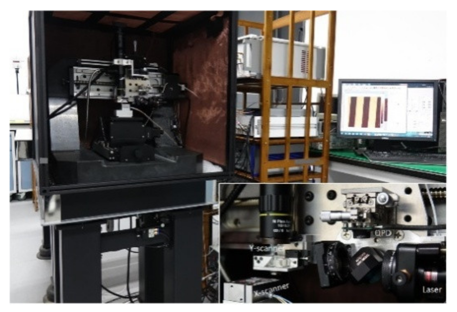
2.1. Homemade High-Speed Atomic Force Microscopy
2.2. Theoretical Analysis of the Installation Errors of the Scanners
2.2.1. X-Scanner
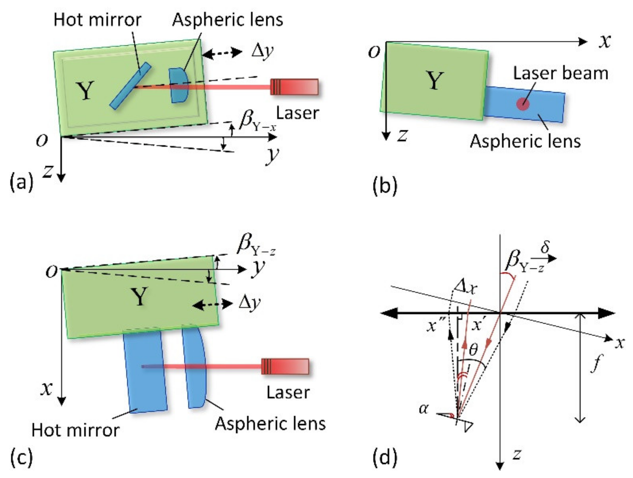
2.2.2. Y-Scanner
2.2.3. Z-Scanner
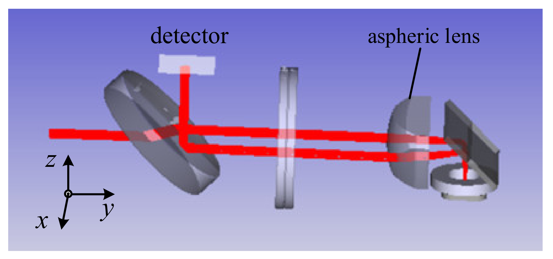
3. Optical Simulation
3.1. Y-Scanner
3.2. Z-Scanner
4. Experiments and Results
5. Conclusions
Author Contributions
Funding
Institutional Review Board Statement
Informed Consent Statement
Data Availability Statement
Conflicts of Interest
References
- Yacoot, A.; Koenders, L. Recent developments in dimensional nanometrology using AFMs. Meas. Sci. Technol. 2011, 22, 122001. [Google Scholar] [CrossRef]
- Wu, S.; Fu, X.; Hu, X.; Hu, X. Manipulation and behavior modeling of one-dimensional nanomaterials on a structured surface. Appl. Surf. Sci. 2010, 256, 4738–4744. [Google Scholar] [CrossRef]
- Reifenberger, R.G. Fundamentals of Atomic Force Microscopy; Part I: Foundations; World Scientific Publishing Company Pte Limited: Singapore, 2016. [Google Scholar]
- Liu, W.; Guo, Y.; Wang, K.; Zhou, X.; Wang, Y.; Lü, J.; Shao, Z.; Hu, J.; Czajkowsky, D.M.; Li, B. Atomic force microscopy-based single-molecule force spectroscopy detects DNA base mismatches. Nanoscale 2019, 11, 17206–17210. [Google Scholar] [CrossRef]
- Matusovsky, O.S.; Kodera, N.; Maceachen, C.; Ando, T.; Cheng, Y.S.; Rassier, D.E. Millisecond Conformational Dynamics of Skeletal Myosin II Power Stroke Studied by High-Speed Atomic Force Microscopy. ACS Nano 2020, 15, 2229–2239. [Google Scholar] [CrossRef]
- Wang, S.; Liu, Q.; Zhao, C.; Lv, F.; Qin, X.; Du, H.; Kang, F.; Li, B. Advances in Understanding Materials for Rechargeable Lithium Batteries by Atomic Force Microscopy. Energy Environ. Mater. 2018, 1, 28–40. [Google Scholar] [CrossRef]
- Liu, Z.; Bi, Z.; Shang, Y.; Loang, Y.; Yang, P.; Li, X.; Zhang, C.; Shang, G. Development of electrochemical high-speed atomic force microscopy for visualizing dynamic processes of battery electrode materials. Rev. Sci. Instrum. 2020, 91, 103701. [Google Scholar] [CrossRef] [PubMed]
- García, R. Amplitude Modulation Atomic Force Microscopy; Wiley-VCH: Weinheim, Germany, 2010. [Google Scholar]
- Yang, W.; Yang, X.; Lu, W.; Yu, N.; Chen, L.; Zhou, L.; Chang, S. A Novel White Light Interference Based AFM Head. J. Lightwave Technol. 2017, 35, 3604–3610. [Google Scholar] [CrossRef]
- Hu, C.; Liu, X.; Yang, W.; Lu, W.; Yu, N.; Chang, S. Improved zero-order fringe positioning algorithms in white light interference based atomic force microscopy. Opt. Lasers Eng. 2018, 100, 71–76. [Google Scholar] [CrossRef]
- Morita, S. Atom world based on nano-forces: 25 years of atomic force microscopy. J. Electron. Microsc. 2011, 60 (Suppl. 1), S199–S211. [Google Scholar] [CrossRef]
- Shiba, Y.; Ono, T.; Minami, K.; Esashi, M. Capacitive AFM Probe for High Speed Imaging. IEEJ Trans. Sens. Micromach. 1998, 118, 5. [Google Scholar] [CrossRef][Green Version]
- Uchihashi, T.; Watanabe, H.; Fukuda, S.; Shibata, M.; Ando, T. Functional extension of high-speed AFM for wider biological applications. Ultramicroscopy 2016, 160, 182–196. [Google Scholar] [CrossRef] [PubMed]
- Fukuda, S.; Uchihashi, T.; Ando, T. Method of mechanical holding of cantilever chip for tip-scan high-speed atomic force microscope. Rev. Sci. Instrum. 2015, 86, 063703. [Google Scholar] [CrossRef] [PubMed]
- Hwang, I.S.; Hung, S.K.; Fu, L.C.; Lin, M.Y. Beam Tracking System for Scanning-Probe Type Atomic Force Microscope. U.S. Patent No. 7,249,494, 31 July 2007. [Google Scholar]
- Aksel, E.; Jones, J.L. Advances in Lead-Free Piezoelectric Materials for Sensors and Actuators. Sensors 2010, 10, 1935–1954. [Google Scholar] [CrossRef]
- Kholkin, A. Piezoelectric Materials and Devices: Applications in Engineering and Medical Sciences; CRC Press/Taylor & Francis: Boca Raton, FL, USA, 2013. [Google Scholar]
- Bhikkaji, B.; Ratnam, M.; Fleming, A.J.; Moheimani, S.O.R. High-Performance Control of Piezoelectric Tube Scanners. IEEE Trans. Control Syst. Technol. 2007, 15, 853–866. [Google Scholar] [CrossRef]
- Moheimani, S.O. Invited review article: Accurate and fast nanopositioning with piezoelectric tube scanners: Emerging trends and future challenges. Rev. Sci. Instrum. 2008, 79, 071101. [Google Scholar] [CrossRef] [PubMed]
- Schitter, G.; Astrom, K.J.; DeMartini, B.E.; Thurner, P.J.; Turner, K.L.; Hansma, P.K. Design and modeling of a high-speed AFM-scanner. IEEE Trans. Control Syst. Technol. 2007, 15, 906–915. [Google Scholar] [CrossRef]
- Cai, W.; Liu, Z.; Chen, Y.; Shang, G. A Mini Review of the Key Components used for the Development of High-Speed Atomic Force Microscopy. Sci. Adv. Mater. 2017, 9, 77–88. [Google Scholar] [CrossRef]
- Dufrêne, Y.; Ando, T.; Garcia, R.; Alsteens, Y.F.D.D.; Martinez-Martin, D.; Engel, A.; Gerber, C.; Muller, D.J. Imaging modes of atomic force microscopy for application in molecular and cell biology. Nat. Nanotechnol. 2017, 12, 295–307. [Google Scholar] [CrossRef]
- Jordan, T.L.; Ounaies, Z. Piezoelectric Ceramics Characterization; ICASE Report; National Aeronautics and Space Administration (NASA): Hanover, MD, USA, 2001; p. 28.
- Kim, H.S.; Kim, J.-H.; Kim, J. A review of piezoelectric energy harvesting based on vibration. Int. J. Precis. Eng. Manuf. 2011, 12, 1129–1141. [Google Scholar] [CrossRef]
- Zhang, M.-H.; Wang, K.; Zhou, J.-S.; Zhou, J.-J.; Chu, X.; Lv, X.; Wu, J.; Li, J. Thermally stable piezoelectric properties of (K, Na)NbO3-based lead-free perovskite with rhombohedral-tetragonal coexisting phase. Acta Mater. 2017, 122, 344–351. [Google Scholar] [CrossRef]
- Li, Y.S.; Ren, J.H.; Feng, W.J. Bending of sinusoidal functionally graded piezoelectric plate under an in-plane magnetic field. Appl. Math. Model. 2017, 47, 63–75. [Google Scholar] [CrossRef]
- Ehmke, M.C.; Schader, F.H.; Webber, K.G.; Rödel, J.; Blendell, J.E.; Bowman, K.J. Stress, temperature and electric field effects in the lead-free (Ba,Ca)(Ti,Zr)O 3 piezoelectric system. Acta Mater. 2014, 78, 37–45. [Google Scholar] [CrossRef]
- Liu, L.; Wu, S.; Pang, H.; Hu, X.; Hu, X. High-speed atomic force microscope with a combined tip-sample scanning architecture. Rev. Sci. Instrum. 2019, 90, 063707. [Google Scholar] [CrossRef] [PubMed]
- Liu, L.; Wu, S.; Wang, Y.Y.; Hu, X.D.; Hu, X.T. Adaptive velocity-dependent proportional-integral controller for high-speed atomic force microscopy. J. Microsc. 2019, 275, 107–114. [Google Scholar] [CrossRef] [PubMed]


Publisher’s Note: MDPI stays neutral with regard to jurisdictional claims in published maps and institutional affiliations. |
© 2021 by the authors. Licensee MDPI, Basel, Switzerland. This article is an open access article distributed under the terms and conditions of the Creative Commons Attribution (CC BY) license (https://creativecommons.org/licenses/by/4.0/).
Share and Cite
Liu, L.; Kong, M.; Wu, S.; Xu, X.; Wang, D. Error Analysis of the Combined-Scan High-Speed Atomic Force Microscopy. Sensors 2021, 21, 6139. https://doi.org/10.3390/s21186139
Liu L, Kong M, Wu S, Xu X, Wang D. Error Analysis of the Combined-Scan High-Speed Atomic Force Microscopy. Sensors. 2021; 21(18):6139. https://doi.org/10.3390/s21186139
Chicago/Turabian StyleLiu, Lu, Ming Kong, Sen Wu, Xinke Xu, and Daodang Wang. 2021. "Error Analysis of the Combined-Scan High-Speed Atomic Force Microscopy" Sensors 21, no. 18: 6139. https://doi.org/10.3390/s21186139
APA StyleLiu, L., Kong, M., Wu, S., Xu, X., & Wang, D. (2021). Error Analysis of the Combined-Scan High-Speed Atomic Force Microscopy. Sensors, 21(18), 6139. https://doi.org/10.3390/s21186139