
Spiral SAR Imaging with Fast Factorized Back-Projection: A Phase Error Analysis

 ,
,
Abstract
:1. Introduction
2. Materials and Methods
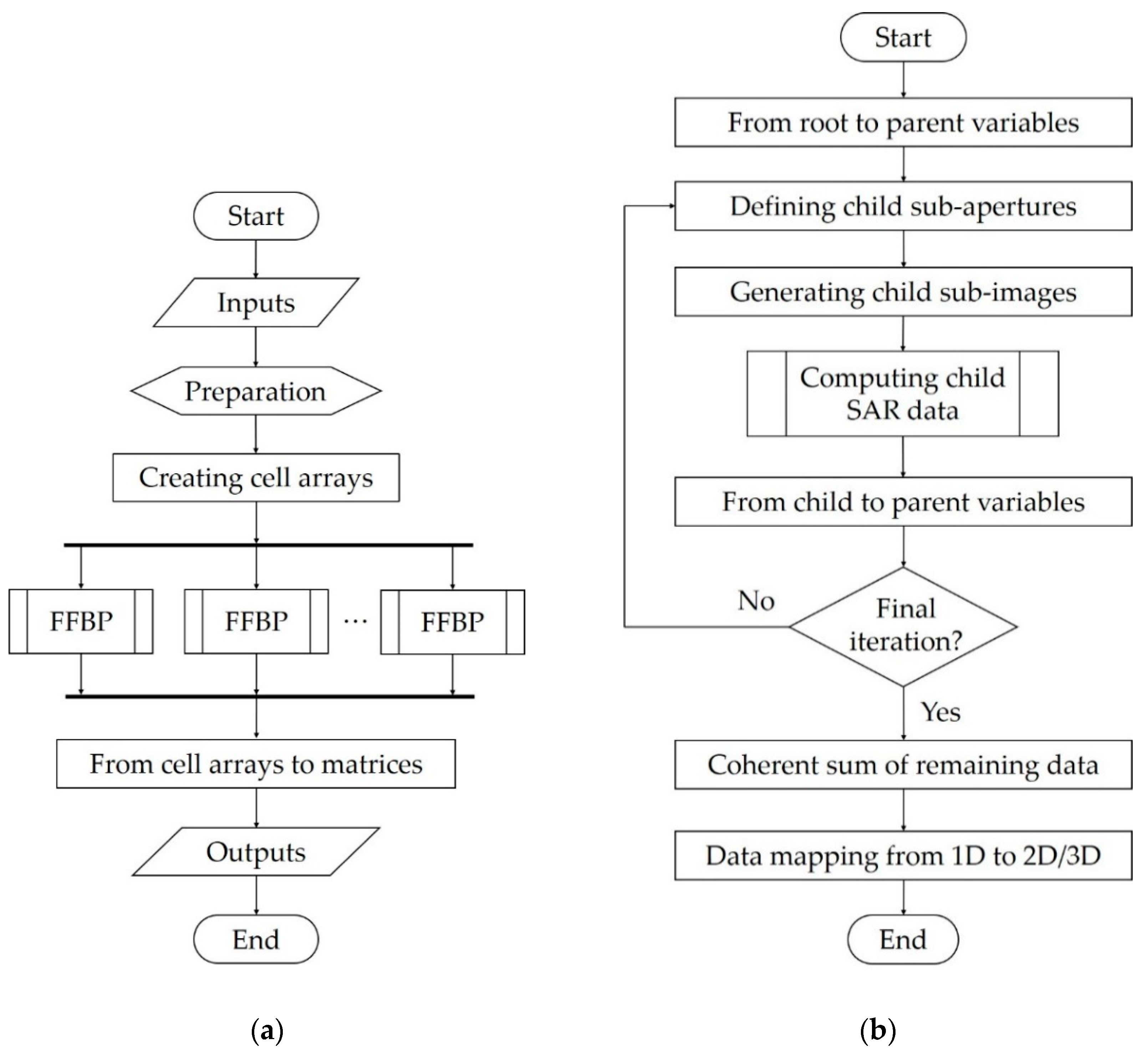
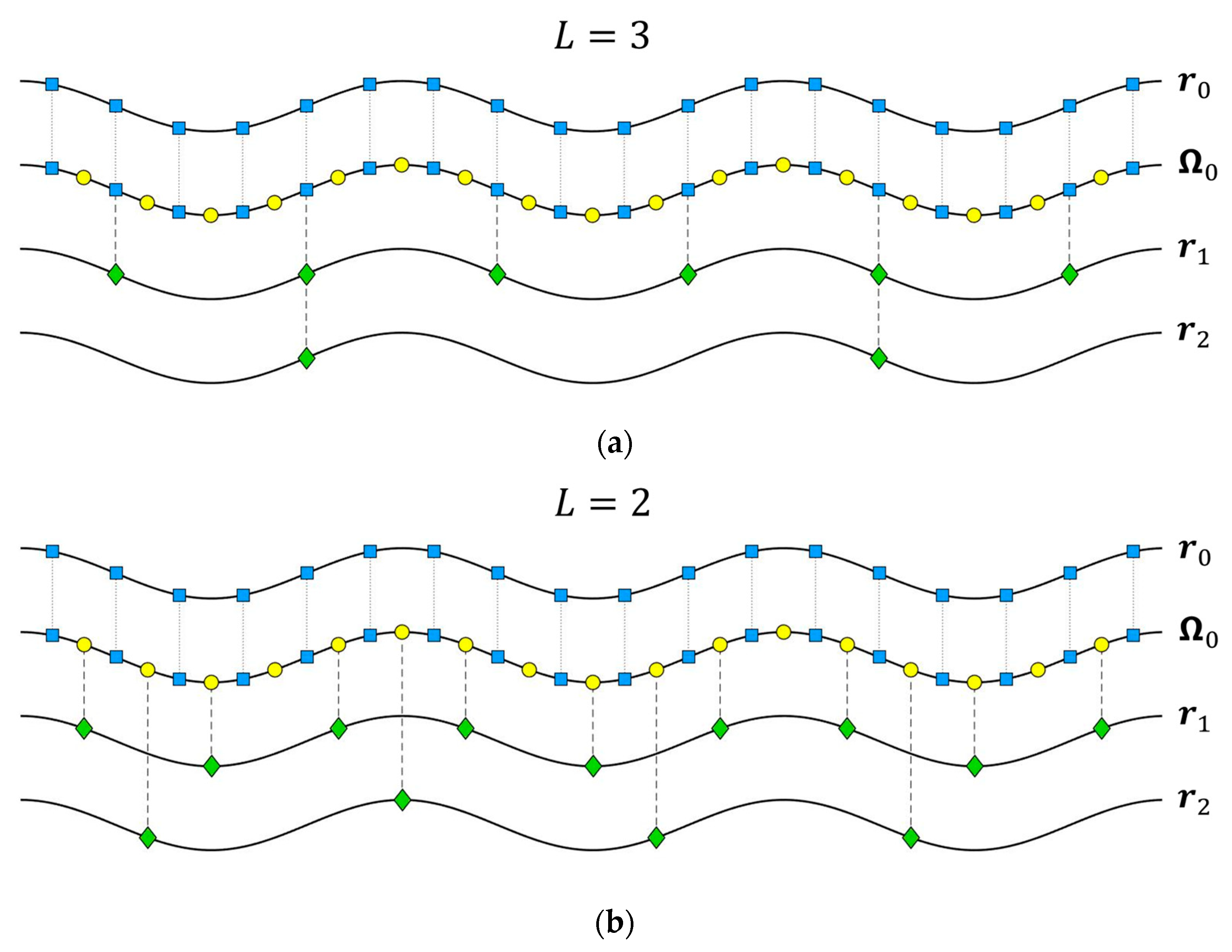
2.1. Fast Factorized Back-Projection Algorithm
- Root variables: either inputs to the algorithm or defined in the preparation step;
- Child variables: calculated within each FFBP iteration and then become parent variables at the end of the iteration;
- Parent variables: inputs to the current iteration.
2.1.1. Defining Child Subapertures
2.1.2. Generating Child Subimages
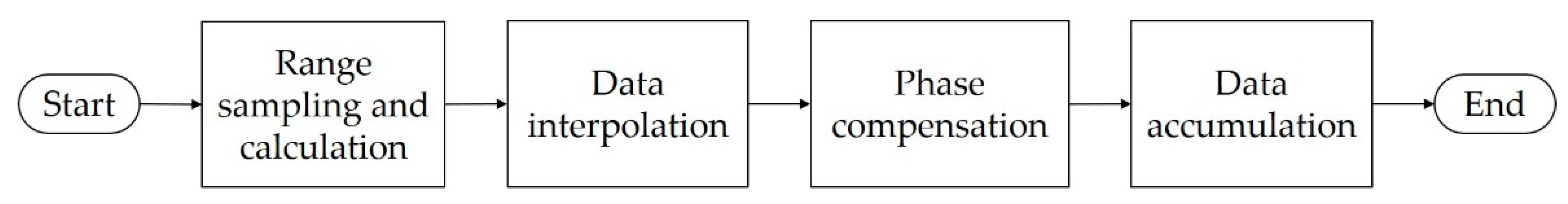
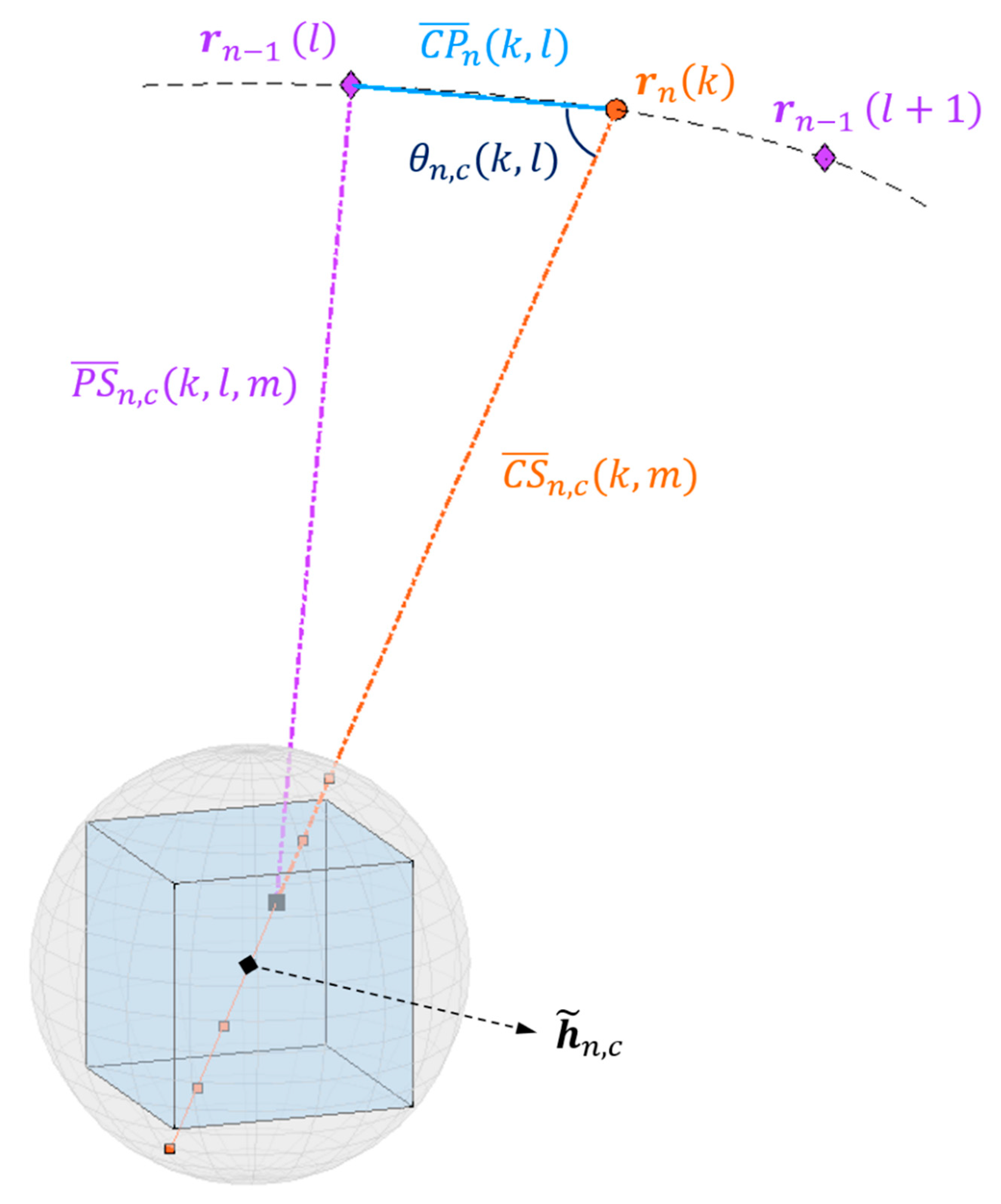
2.1.3. Computing Child SAR Data
- (C) the child subaperture center ;
- (P) the parent subaperture center ;
- (S) the th data sample within a child subimage centered at .
2.2. The Phase Error Hypothesis
- Calculate the maximum subimage size for the first iteration;
- Balance the increase in subaperture length with an equivalent decrease in subimage width to keep the range error constant.
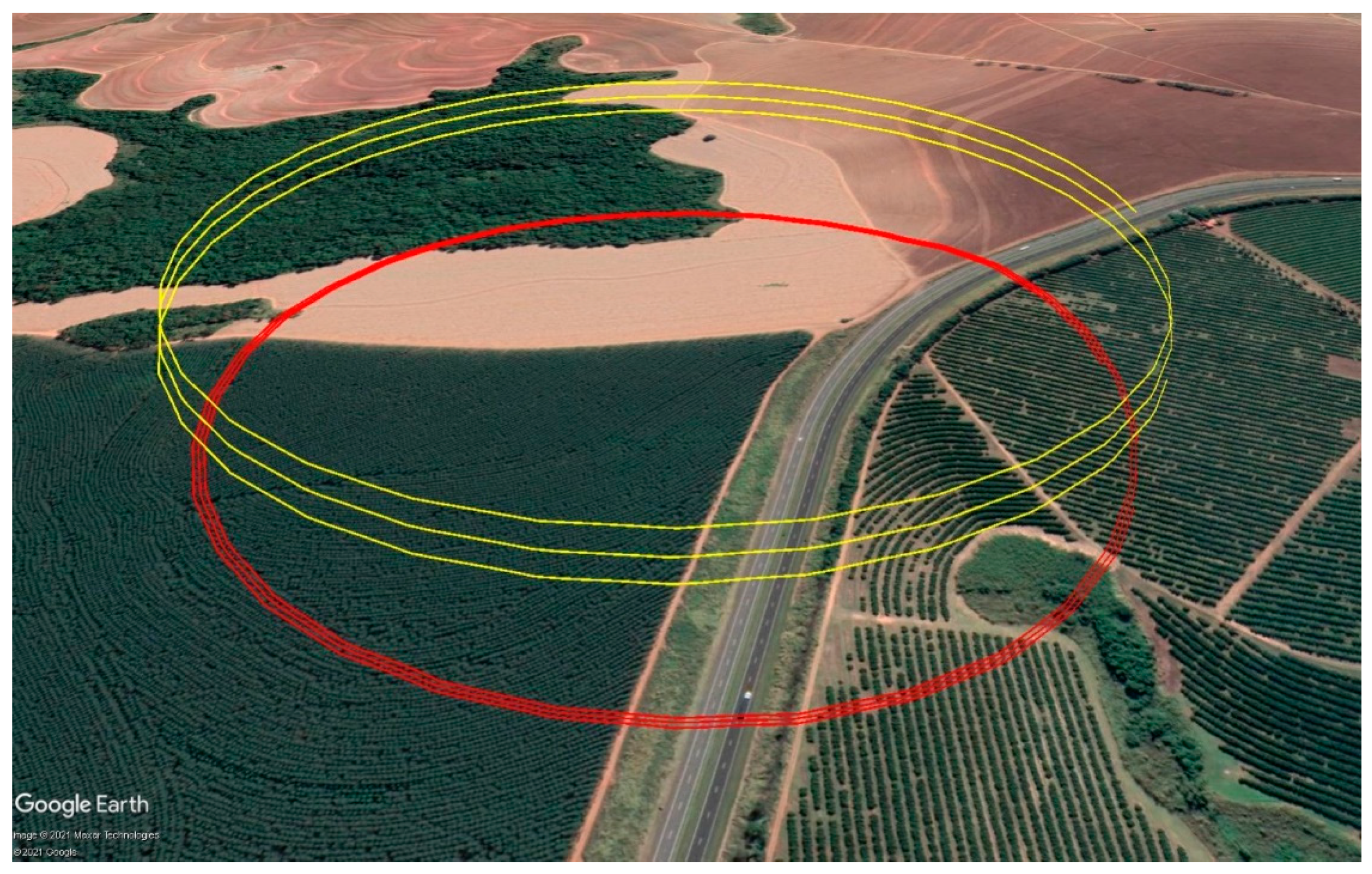
2.3. The Case Study
- Setting different values for the number of subapertures that are combined at each iteration ();
- Choosing different schemes for the initial partition into image blocks;
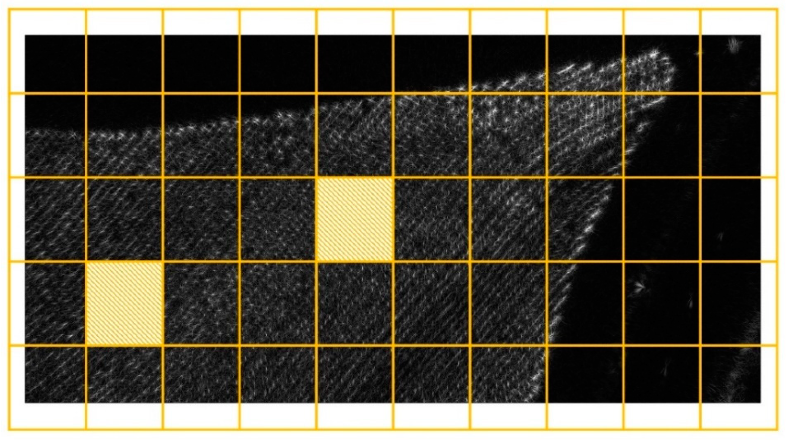
- Selecting two image blocks for analysis, one close to the edge and one close to the center of the output image (see Figure 8).
3. Results
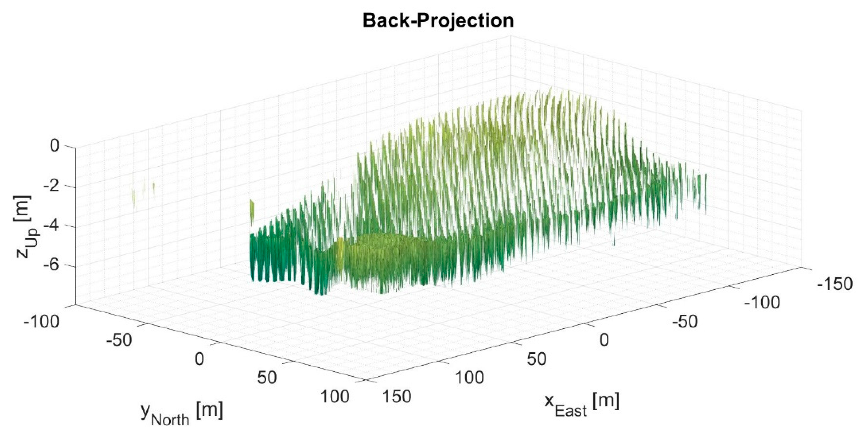
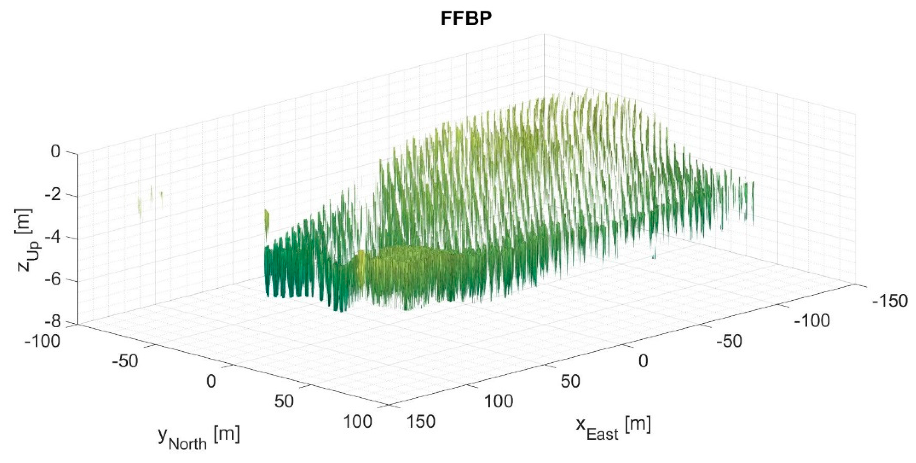
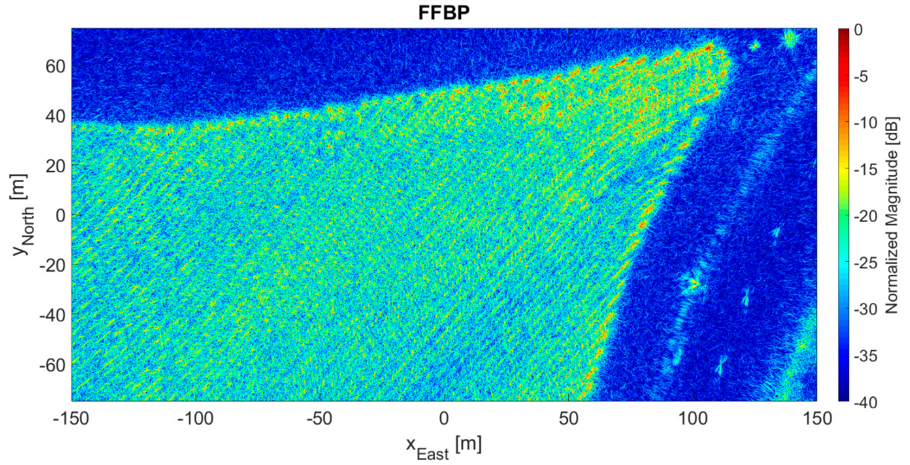
3.1. FFBP vs. BP
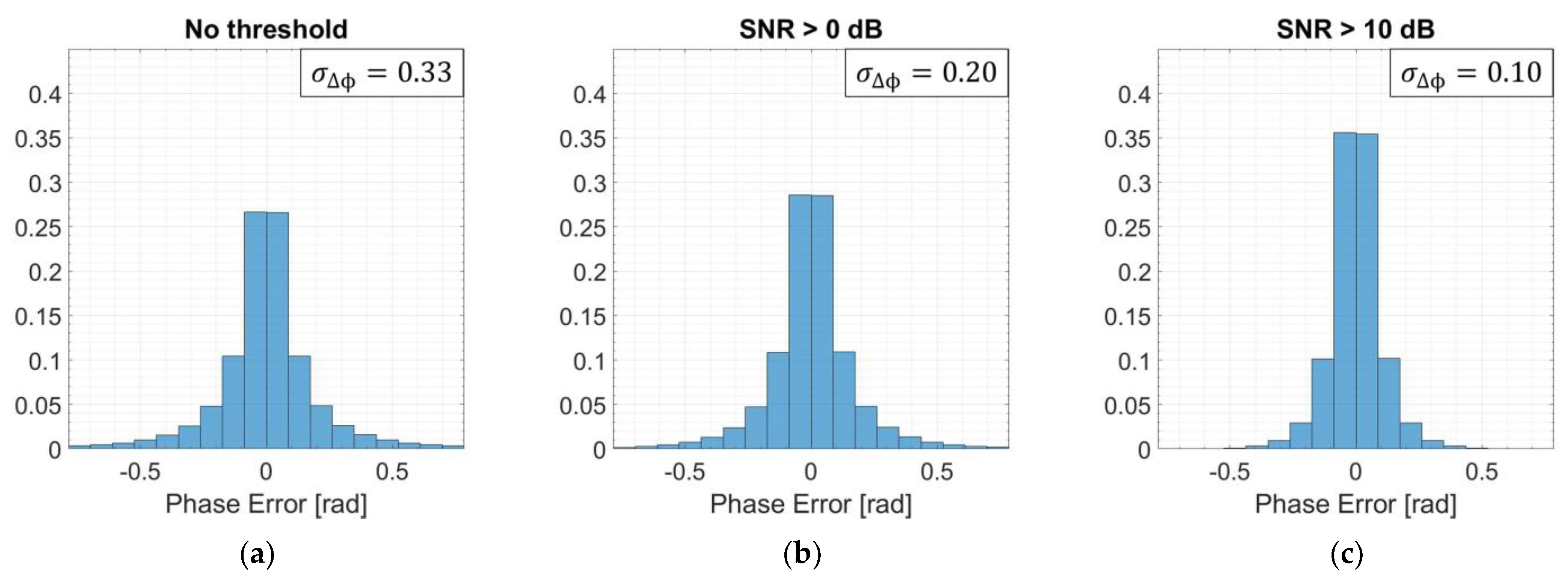
3.2. Phase Error vs. SNR
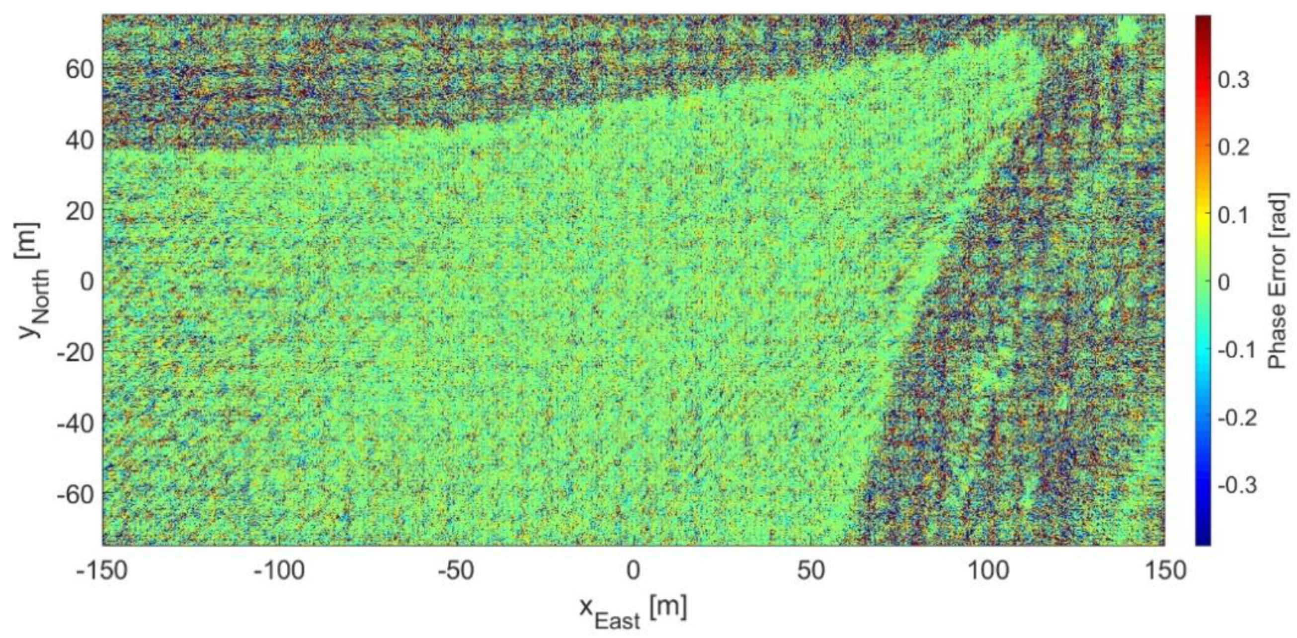
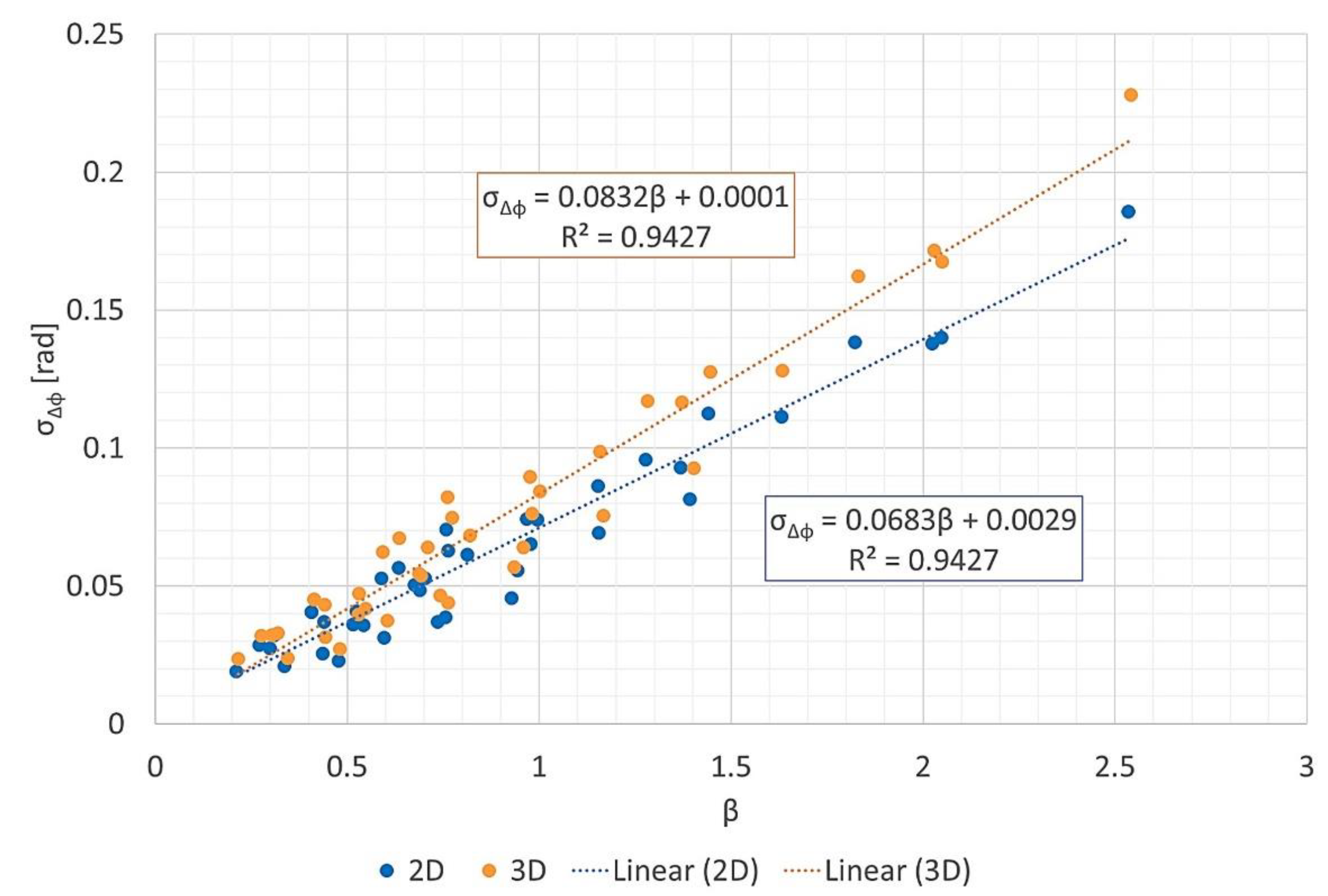
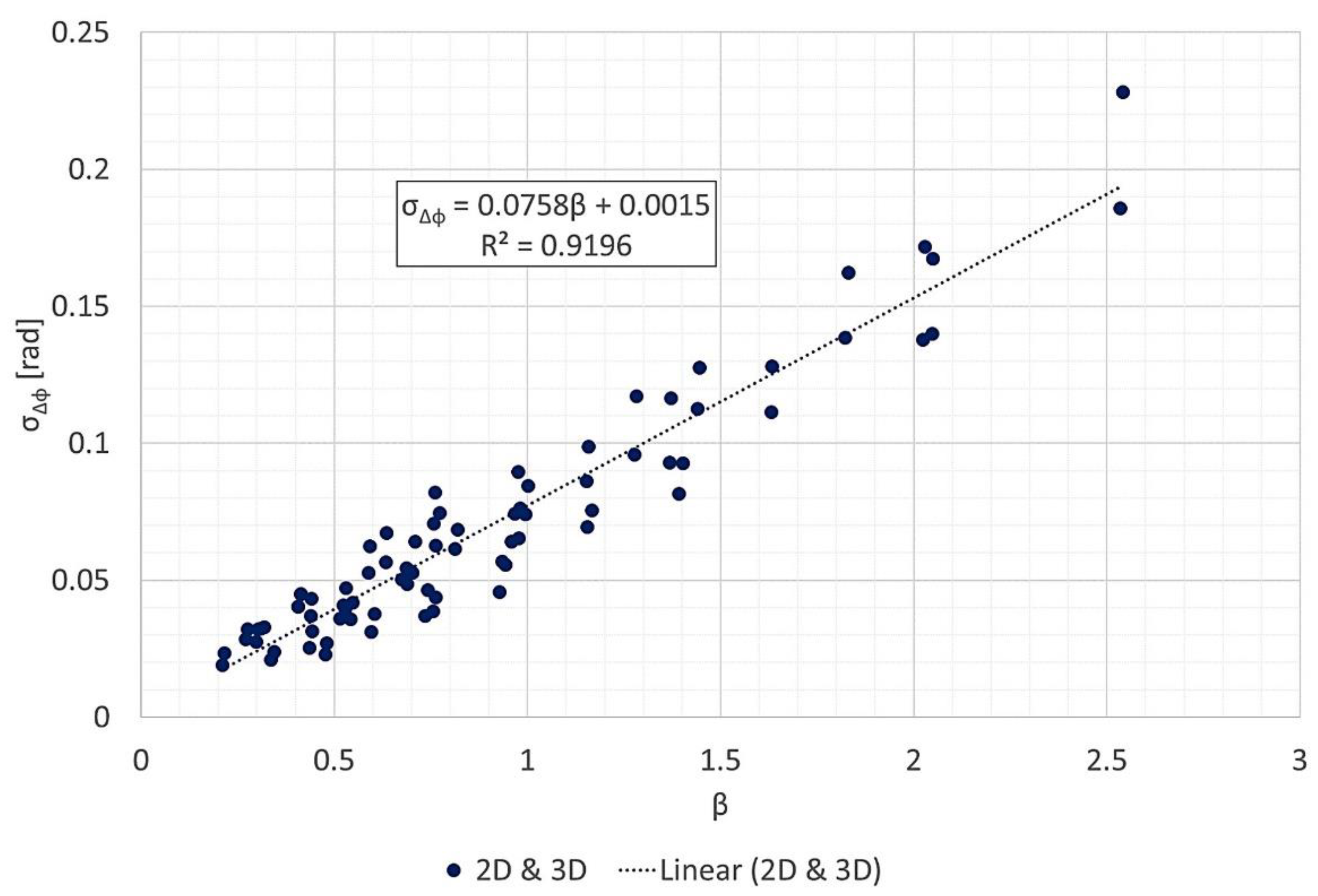
3.3. Phase Error vs. Geometric Parameters
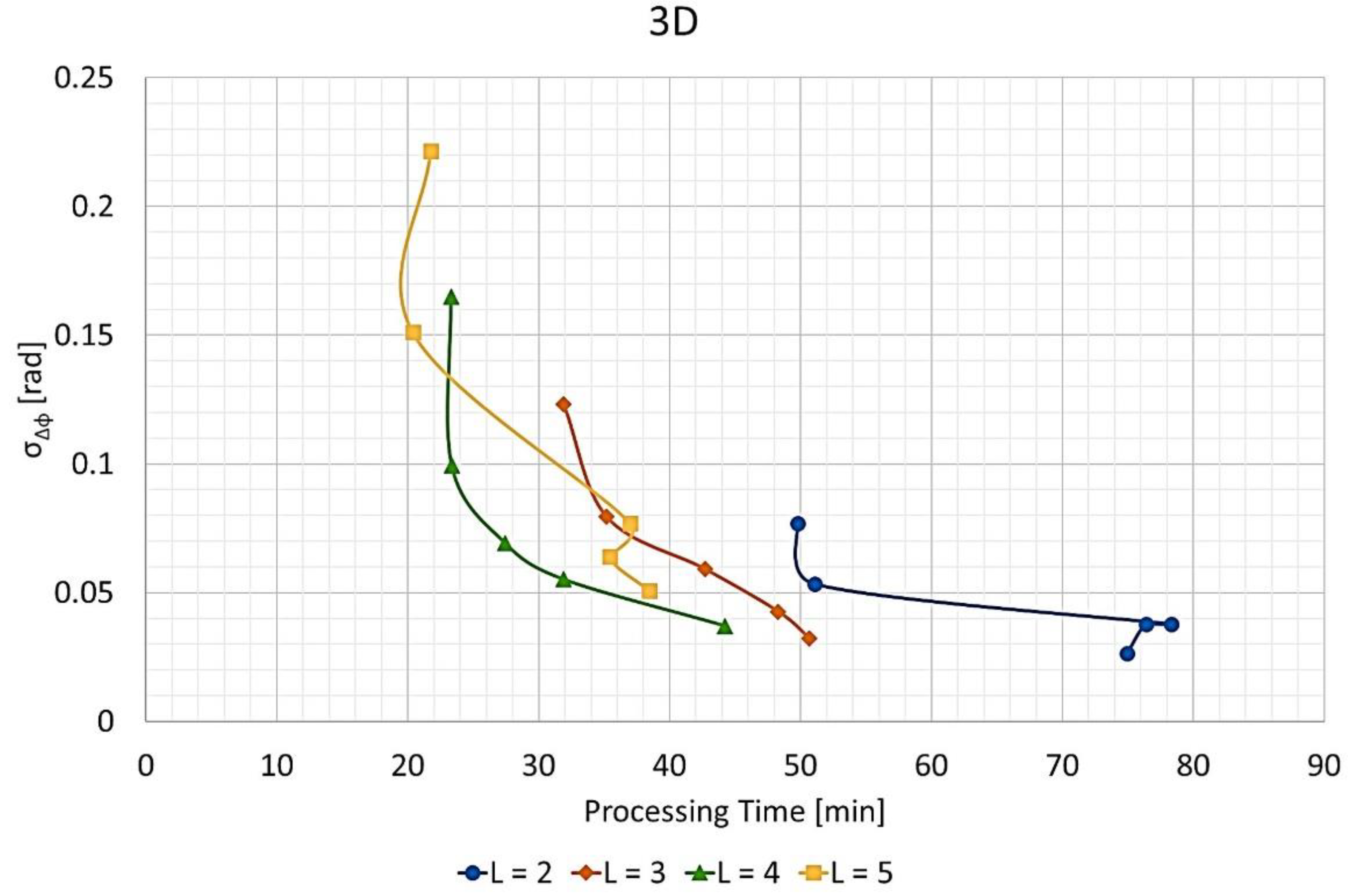
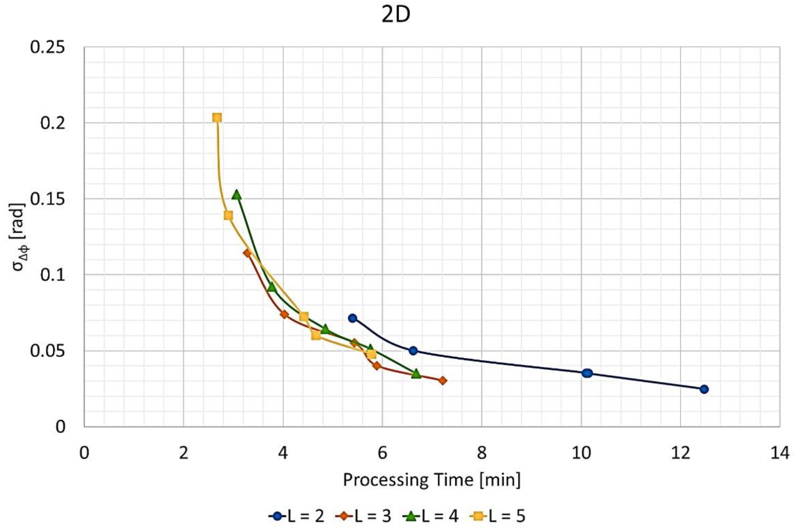
3.4. Phase Error vs. Time
4. Discussion
- 5 with a (16 × 8 × 1) initial partition for 2D;
- 2 with an (8 × 4 × 1) initial partition for 3D.
5. Conclusions
Author Contributions
Funding
Data Availability Statement
Acknowledgments
Conflicts of Interest
References
- Ishimaru, A.; Chan, T.-K.; Kuga, Y. An Imaging Technique Using Confocal Circular Synthetic Aperture Radar. IEEE Trans. Geosci. Remote Sens. 1998, 36, 1524–1530. [Google Scholar] [CrossRef]
- Ponce, O.; Prats-Iraola, P.; Pinheiro, M.; Rodriguez-Cassola, M.; Scheiber, R.; Reigber, A.; Moreira, A. Fully Polarimetric High-Resolution 3-D Imaging with Circular SAR at L-Band. IEEE Trans. Geosci. Remote Sens. 2013, 52, 3074–3090. [Google Scholar] [CrossRef]
- Moore, L.; Potter, L.; Ash, J. Three-Dimensional Position Accuracy in Circular Synthetic Aperture Radar. IEEE Aerosp. Electron. Syst. Mag. 2014, 29, 29–40. [Google Scholar] [CrossRef]
- Ponce, O.; Prats-Iraola, P.; Scheiber, R.; Reigber, A.; Moreira, A. First Airborne Demonstration of Holographic SAR Tomography with Fully Polarimetric Multicircular Acquisitions at L-Band. IEEE Trans. Geosci. Remote Sens. 2016, 54, 6170–6196. [Google Scholar] [CrossRef]
- Zhu, S.; Zhang, Z.; Liu, B.; Yu, W. Three-Dimensional High Resolution Imaging Method of Multi-Pass Circular SAR Based on Joint Sparse Model. In Proceedings of the EUSAR 2016: 11th European Conference on Synthetic Aperture Radar, Hamburg, Germany, 6–9 June 2016; pp. 1–5. [Google Scholar]
- Bao, Q.; Lin, Y.; Hong, W.; Shen, W.; Zhao, Y.; Peng, X. Holographic SAR Tomography Image Reconstruction by Combination of Adaptive Imaging and Sparse Bayesian Inference. IEEE Geosci. Remote Sens. Lett. 2017, 14, 1248–1252. [Google Scholar] [CrossRef]
- Farhadi, M.; Jie, C. Distributed Compressive Sensing for Multi-Baseline Circular SAR Image Formation. In Proceedings of the 2017 IEEE International Conference on Imaging Systems and Techniques (IST), Beijing, China, 18–20 October 2017; pp. 1–6. [Google Scholar]
- Feng, D.; An, D.; Huang, X.; Zhou, Z. Holographic SAR Tomographic Processing of the Multicircular Data. In Proceedings of the 2018 Asia-Pacific Microwave Conference (APMC), Kyoto, Japan, 6–9 November 2018; pp. 830–832. [Google Scholar]
- Feng, D.; An, D.; Chen, L.; Huang, X.; Zhou, Z. Multicircular SAR 3-D Imaging Based on Iterative Adaptive Approach. In Proceedings of the 2019 6th Asia-Pacific Conference on Synthetic Aperture Radar (APSAR), Xiamen, China, 26–29 November 2019; pp. 1–5. [Google Scholar]
- Lv, C.; Deng, B.; Zhang, Y.; Yang, Q.; Wang, H. Terahertz Spiral SAR Imaging Algorithms and Simulations. In Proceedings of the 2020 IEEE 4th Information Technology, Networking, Electronic and Automation Control Conference (ITNEC), Chongqing, China, 12–14 June 2020; Volume 1, pp. 1746–1750. [Google Scholar]
- McCorkle, J.W.; Rofheart, M. Order N2 Log(N) Backprojector Algorithm for Focusing Wide-Angle Wide-Bandwidth Arbitrary-Motion Synthetic Aperture Radar. In Proceedings of the Radar Sensor Technology; International Society for Optics and Photonics, Orlando, FL, USA, 17 June 1996; Volume 2747, pp. 25–36. [Google Scholar]
- Ulander, L.M.H.; Hellsten, H.; Stenstrom, G. Synthetic-Aperture Radar Processing Using Fast Factorized Back-Projection. IEEE Trans. Aerosp. Electron. Syst. 2003, 39, 760–776. [Google Scholar] [CrossRef] [Green Version]
- Zhang, H.; Tang, J.; Wang, R.; Deng, Y.; Wang, W.; Li, N. An Accelerated Backprojection Algorithm for Monostatic and Bistatic SAR Processing. Remote Sens. 2018, 10, 140. [Google Scholar] [CrossRef] [Green Version]
- Liang, D.; Zhang, H.; Fang, T.; Lin, H.; Liu, D.; Jia, X. A Modified Cartesian Factorized Backprojection Algorithm Integrating with Non-Start-Stop Model for High Resolution SAR Imaging. Remote Sens. 2020, 12, 3807. [Google Scholar] [CrossRef]
- Zhang, M.; Li, H.; Wang, G. High-Precision Spotlight SAR Imaging with Joint Modified Fast Factorized Backprojection and Autofocus. Int. J. Antennas Propag. 2020, 2020, e2495050. [Google Scholar] [CrossRef]
- Li, X.; Zhou, S.; Yang, L. A New Fast Factorized Back-Projection Algorithm with Reduced Topography Sensibility for Missile-Borne SAR Focusing with Diving Movement. Remote Sens. 2020, 12, 2616. [Google Scholar] [CrossRef]
- Song, X.; Yu, W. Processing Video-SAR Data with the Fast Backprojection Method. IEEE Trans. Aerosp. Electron. Syst. 2016, 52, 2838–2848. [Google Scholar] [CrossRef]
- Xie, H.; Shi, S.; An, D.; Wang, G.; Wang, G.; Xiao, H.; Huang, X.; Zhou, Z.; Xie, C.; Wang, F.; et al. Fast Factorized Backprojection Algorithm for One-Stationary Bistatic Spotlight Circular SAR Image Formation. IEEE J. Sel. Top. Appl. Earth Obs. Remote Sens. 2017, 10, 1494–1510. [Google Scholar] [CrossRef]
- Guo, Z.; Zhang, H.; Ye, S. Cartesian Based FFBP Algorithm for Circular SAR Using NUFFT Interpolation. In Proceedings of the 2019 6th Asia-Pacific Conference on Synthetic Aperture Radar (APSAR), Xiamen, China, 26–29 November 2019; pp. 1–5. [Google Scholar]
- Góes, J.A.; Castro, V.; Sant’Anna Bins, L.; Hernandez-Figueroa, H.E. 3D Fast Factorized Back-Projection in Cartesian Coordinates. In Proceedings of the 2020 IEEE Radar Conference (RadarConf20), Florence, Italy, 21–25 September 2020; pp. 1–6. [Google Scholar]
- Góes, J.A. 3D FFBP; Zenodo: Geneva, Switzerland, 2021. [Google Scholar] [CrossRef]
- Moreira, L.; Castro, F.; Góes, J.A.; Bins, L.; Teruel, B.; Fracarolli, J.; Castro, V.; Alcântara, M.; Oré, G.; Luebeck, D.; et al. A Drone-Borne Multiband DInSAR: Results and Applications. In Proceedings of the 2019 IEEE Radar Conference (RadarConf), Boston, MA, USA, 22–26 April 2019; pp. 1–6. [Google Scholar]
- Moreira, L.; Lübeck, D.; Wimmer, C.; Castro, F.; Góes, J.A.; Castro, V.; Alcântara, M.; Oré, G.; Oliveira, L.P.; Bins, L.; et al. Drone-Borne P-Band Single-Pass InSAR. In Proceedings of the 2020 IEEE Radar Conference (RadarConf20), Florence, Italy, 21–25 September 2020; pp. 1–6. [Google Scholar]
- Morton, G.M. A Computer Oriented Geodetic Data Base and a New Technique in File Sequencing; IBM: Otawa, ON, Canada, 1966; Available online: https://dominoweb.draco.res.ibm.com/reports/Morton1966.pdf (accessed on 26 July 2021).
- Connor, M.; Kumar, P. Fast Construction of K-Nearest Neighbor Graphs for Point Clouds. IEEE Trans. Vis. Comput. Graph. 2010, 16, 599–608. [Google Scholar] [CrossRef] [PubMed] [Green Version]
- Just, D.; Bamler, R. Phase Statistics of Interferograms with Applications to Synthetic Aperture Radar. Appl. Opt. 1994, 33, 4361–4368. [Google Scholar] [CrossRef] [PubMed]


| 0 | 9 | ||||||
| 1 | 10 | ||||||
| 2 | 11 | ||||||
| 3 | 12 | ||||||
| 4 | 13 | ||||||
| 5 | 14 | ||||||
| 6 | 15 | ||||||
| 7 | 16 | ||||||
| 8 | 17 |
| Radar Parameters | Values | Units |
|---|---|---|
| Carrier wavelength | 70.54 | cm |
| Bandwidth | 50 | MHz |
| Range resolution | 2.4 | m |
| Pulse repetition frequency | 64.95 | Hz |
| Mean velocity | 8.5 | m/s |
| Mean flight radius | 338 | m |
| Height above ground level | 79–120 | m |
| Number of turns | 3 | - |
| Processing Parameter | Values | |
|---|---|---|
| Output image dimension | 2D | 300 × 150 m2 |
| 3D | 300 × 150 × 2.4 m3 | |
| Output image resolution | 2D | 0.2 × 0.2 m2 |
| 3D | 0.2 × 0.2 × 0.2 m3 | |
| Number of subapertures combined at each iteration () | 2 | |
| 3 | ||
| 4 | ||
| 5 | ||
| Initial partition of image blocks | 8 × 4 × 1 | |
| 12 × 6 × 1 | ||
| 16 × 8 × 1 | ||
| 20 × 10 × 1 | ||
| 24 × 12 × 1 |
| Data | Coefficient | Estimate | Standard Error | 95% Confidence Interval | p-Value | ||
|---|---|---|---|---|---|---|---|
| 2D | Intercept | 0.0029 | 0.0028 | −0.0029 | 0.0086 | 0.32 | 0.9427 |
| Slope | 0.0683 | 0.0027 | 0.0628 | 0.0738 | 3.3 × | ||
| 3D | Intercept | 0.0001 | 0.0035 | −0.0069 | 0.0071 | 0.97 | 0.9427 |
| Slope | 0.0832 | 0.0033 | 0.0765 | 0.0899 | 3.3 × | ||
| 2D and 3D | Intercept | 0.0015 | 0.0026 | −0.0038 | 0.0067 | 0.58 | 0.9196 |
| Slope | 0.0758 | 0.0025 | 0.0708 | 0.0809 | 1.9 × | ||
| Image Type | BP Processing Time | FFBP | ||
|---|---|---|---|---|
| Configuration | Processing Time | Speed-Up Factor | ||
| 2D | Fastest | 2 min 40 s | 13.33 | |
| 35 min 33 s | Average | 5 min 45 s | 6.18 | |
| Slowest | 12 min 28 s | 2.85 | ||
| 3D | Fastest | 20 min 24 s | 21.2 | |
| 7 h 12 min 18 s | Average | 42 min 8 s | 10.3 | |
| Slowest | 1 h 18 min 18 s | 5.52 | ||
| Image Type | Figure of Merit | Image Quality | ||
|---|---|---|---|---|
| Highest | Average | Lowest | ||
| 2D | Phase Error Standard deviation | 0.025 rad (1.4°) | 0.073 rad (4.2°) | 0.20 (11.7°) |
| Degree of coherence | 0.9999 | 0.9993 | 0.9945 | |
| SNR of equivalent Thermal noise | 40 dB | 31 dB | 23 dB | |
| 3D | Phase error Standard deviation | 0.026 (1.5°) | 0.077 rad (4.4°) | 0.22 rad (12.7°) |
| Degree of coherence | 0.9999 | 0.9988 | 0.9921 | |
| SNR of equivalent Thermal noise | 38 dB | 29 dB | 21 dB | |
Publisher’s Note: MDPI stays neutral with regard to jurisdictional claims in published maps and institutional affiliations. |
© 2021 by the authors. Licensee MDPI, Basel, Switzerland. This article is an open access article distributed under the terms and conditions of the Creative Commons Attribution (CC BY) license (https://creativecommons.org/licenses/by/4.0/).
Share and Cite
Góes, J.A.; Castro, V.; Sant’Anna Bins, L.; Hernandez-Figueroa, H.E. Spiral SAR Imaging with Fast Factorized Back-Projection: A Phase Error Analysis. Sensors 2021, 21, 5099. https://doi.org/10.3390/s21155099
Góes JA, Castro V, Sant’Anna Bins L, Hernandez-Figueroa HE. Spiral SAR Imaging with Fast Factorized Back-Projection: A Phase Error Analysis. Sensors. 2021; 21(15):5099. https://doi.org/10.3390/s21155099
Chicago/Turabian StyleGóes, Juliana A., Valquiria Castro, Leonardo Sant’Anna Bins, and Hugo E. Hernandez-Figueroa. 2021. "Spiral SAR Imaging with Fast Factorized Back-Projection: A Phase Error Analysis" Sensors 21, no. 15: 5099. https://doi.org/10.3390/s21155099
APA StyleGóes, J. A., Castro, V., Sant’Anna Bins, L., & Hernandez-Figueroa, H. E. (2021). Spiral SAR Imaging with Fast Factorized Back-Projection: A Phase Error Analysis. Sensors, 21(15), 5099. https://doi.org/10.3390/s21155099