
New Distributed Fibre Optic 3DSensor with Thermal Self-Compensation System: Design, Research and Field Proof Application Inside Geotechnical Structure


Abstract
:1. Introduction
1.1. General Background
- The possibility of analysing the structural behaviour from a real zero state, which is impossible with installed sensors within existing structures with unknown initial levels of stress and or/deformation;
- Integration inside the structure (ground or concrete) providing the more accurate transfer of the measured physical quantity from the structure to the sensor—no additional mounting brackets or installation methods are needed;
- Natural and effective protection of the sensors integrated inside the structure against mechanical damages or harsh environmental conditions. The predicted operation lifetime of such a system is comparable with the operation lifetime of the structure itself.
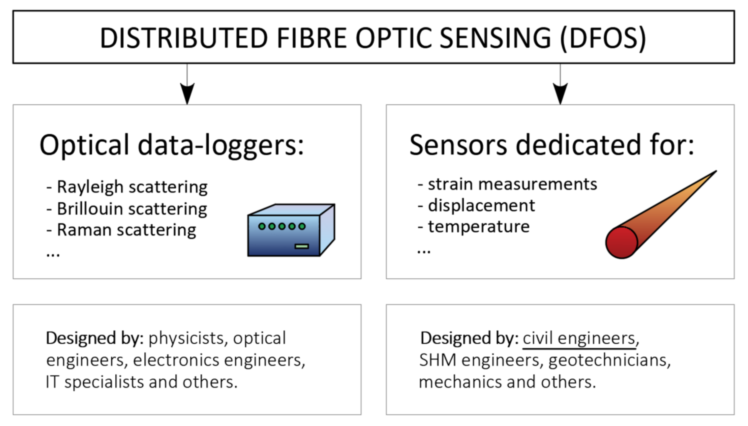
1.2. Distributed Sensing Principles and Sensors
- The linear and elastic behaviour of the structure;
- Homogeneous materials without any discontinuities such as cracks or fractures;
- Accurate strain transfer from the structure to the fibre;
- Appropriate thermal compensation;
- The sufficient precision of sensors’ positioning in field conditions.
2. New Distributed Fibre Optic Displacement Sensor
2.1. Basic Concept and Design Stage
2.2. Data Processing
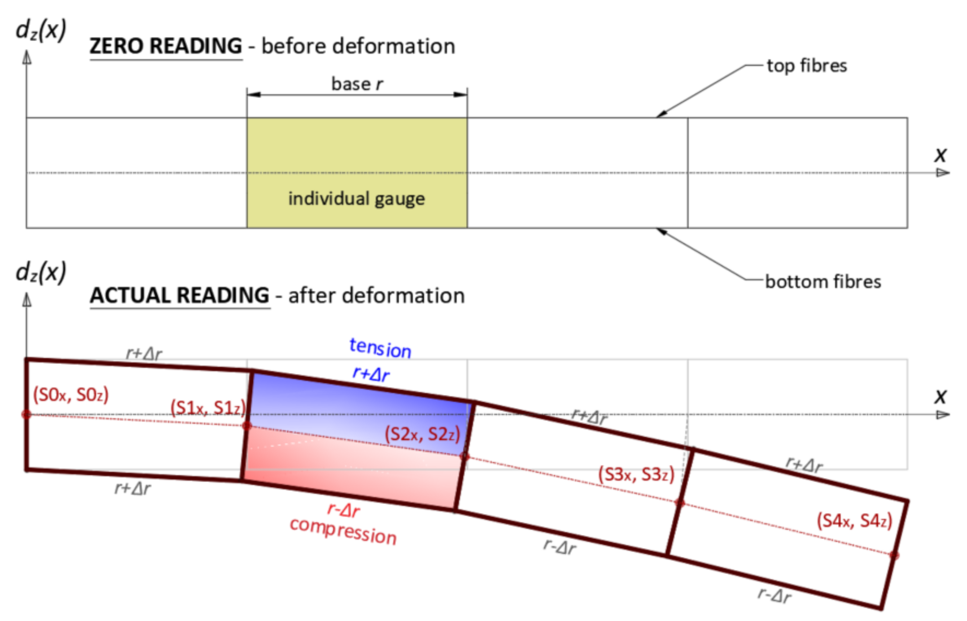
- Sensor’s core works in the elastic range of strains;
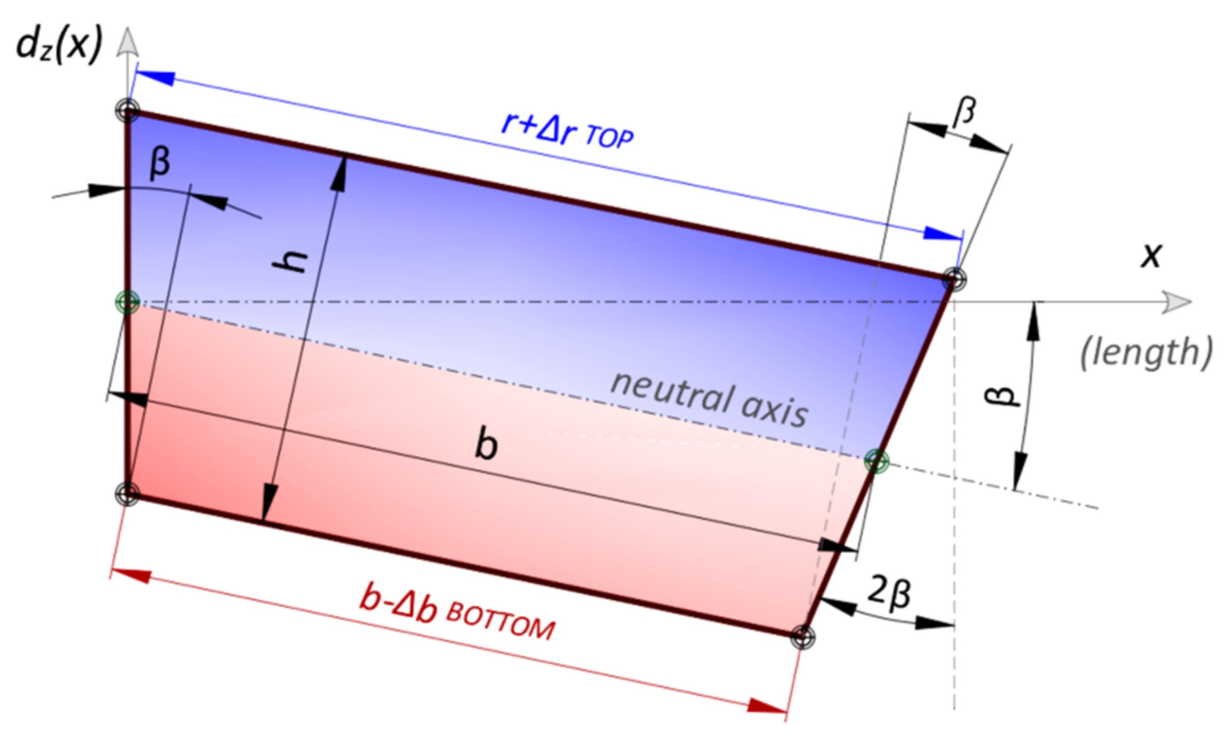
- The Euler–Bernoulli hypotheses that plane sections remain plane and normal to the axis of the sensor’s core;
- The geometry of the core (height and width) and resulting distance between the opposite optical fibres, are constant over length;
- Production tolerances are known (e.g., standard deviation of the height over length) and can be used to assess the final accuracy;
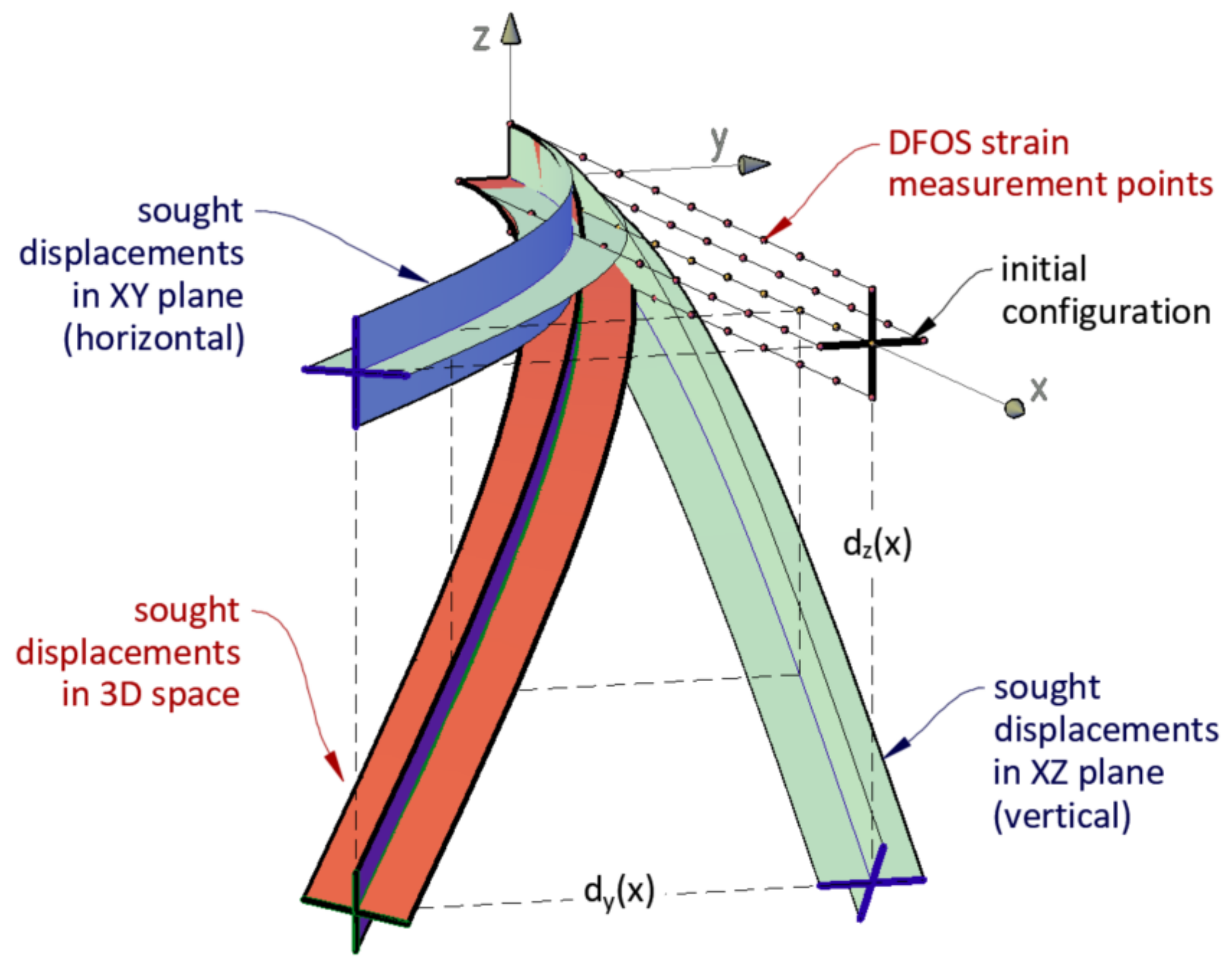
- The superposition principle applies when calculating displacements in 3D space (displacements could be calculated separately for vertical XZ and horizontal plane XY);
- Boundary conditions are known (rotations and displacements in at least one measuring point or displacements in at least two measuring points);
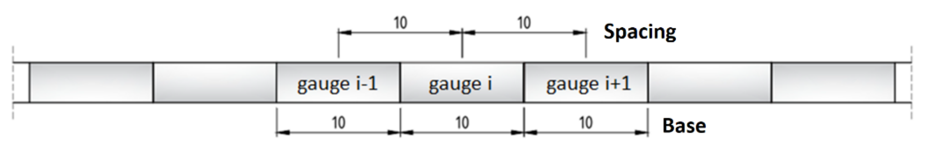
- Strains are measured with defined spatial resolution r (spacing) and with known accuracy provided by the calibration process;
- Strains are averaged over the gauge length equal to the spatial resolution, so that the series of front-connected gauges is created—Figure 7;
- Displacements are calculated in the same fixed points defined by spatial resolution such as in the case of strain measurements (values are linearly interpolated between the points in their simplest terms).
2.3. Thermal Self-Compensation System
2.4. Laboratory Issues
2.5. Ready-to-Use Sensors
2.6. Data Acquisition Systems
3. Laboratory Studies
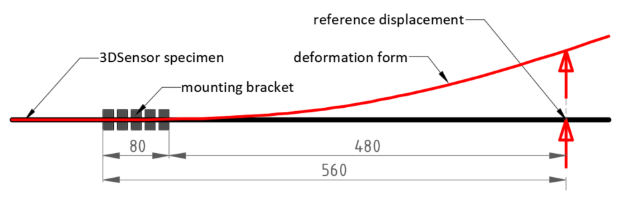
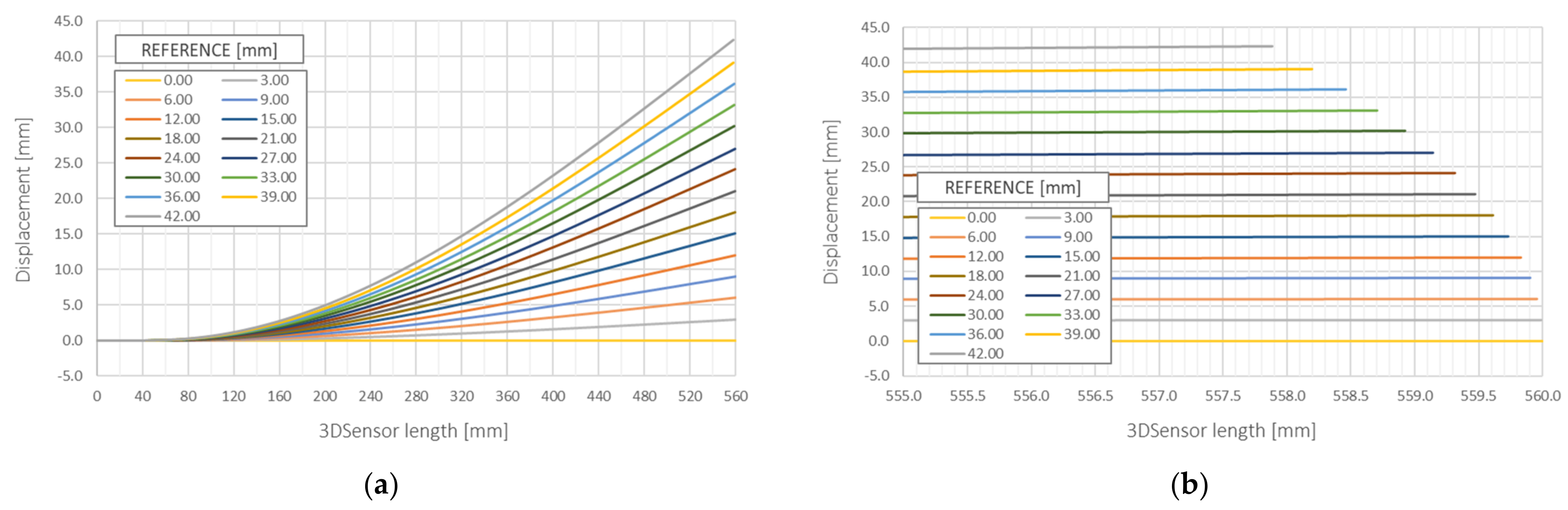
3.1. Cantilever Scheme
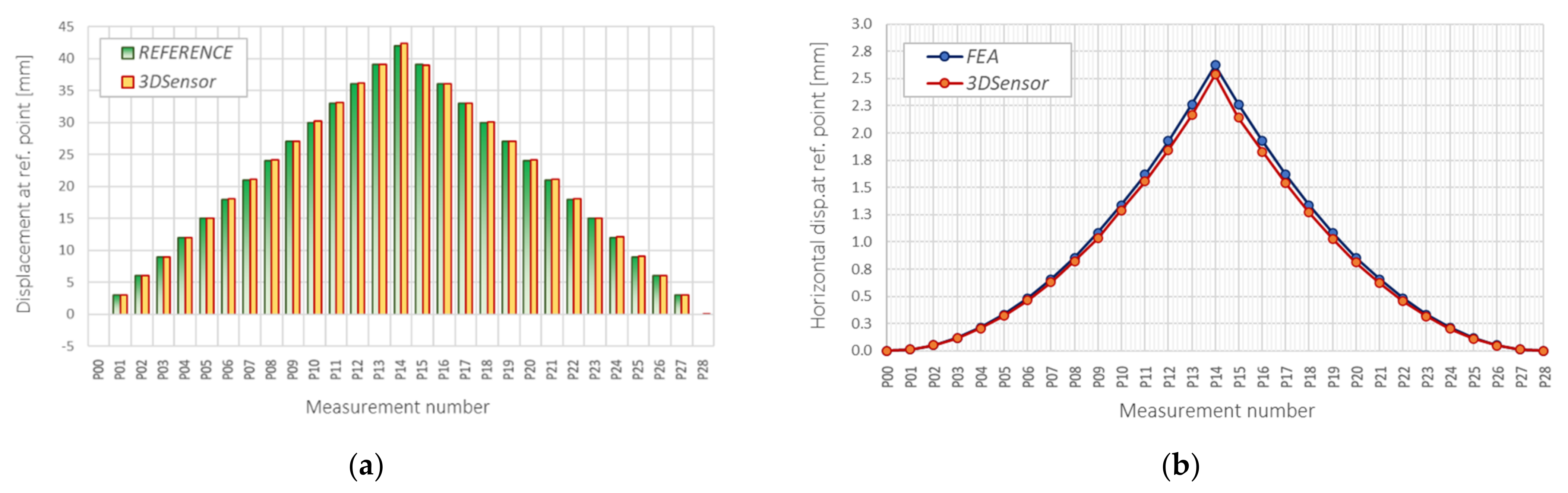
- Micrometres for vertical displacements (Figure 16a); mean absolute and relative errors: 0.077 mm and 0.427%; corresponding standard deviations: 0.076 mm and 0.424%;
- FE analysis for horizontal shortenings (Figure 16b); mean absolute and relative errors: 0.042 mm and 4.707%; corresponding standard deviations: 0.035 mm and 1.049%.
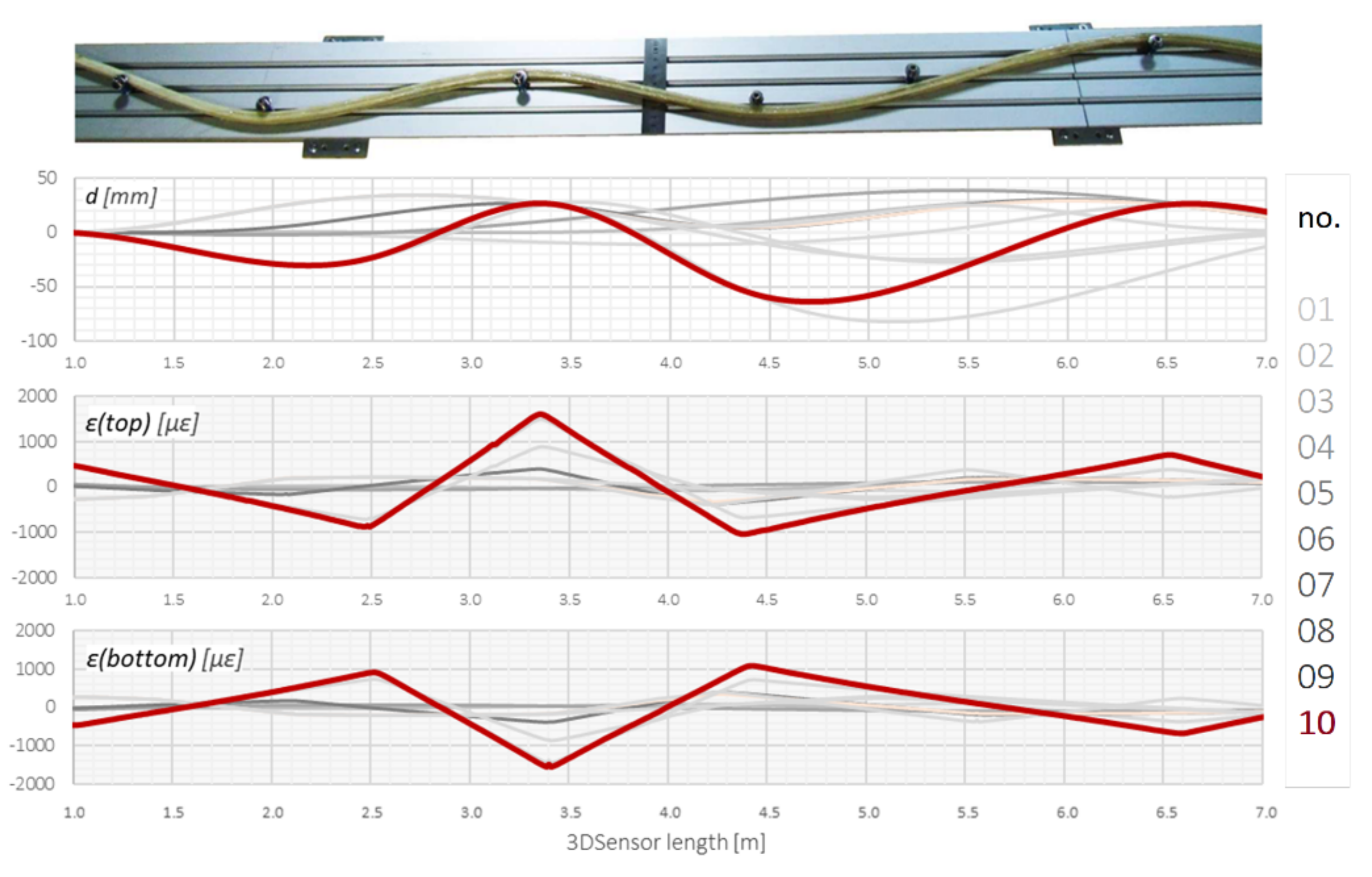
3.2. Simply Supported and Continuous Beam Scheme
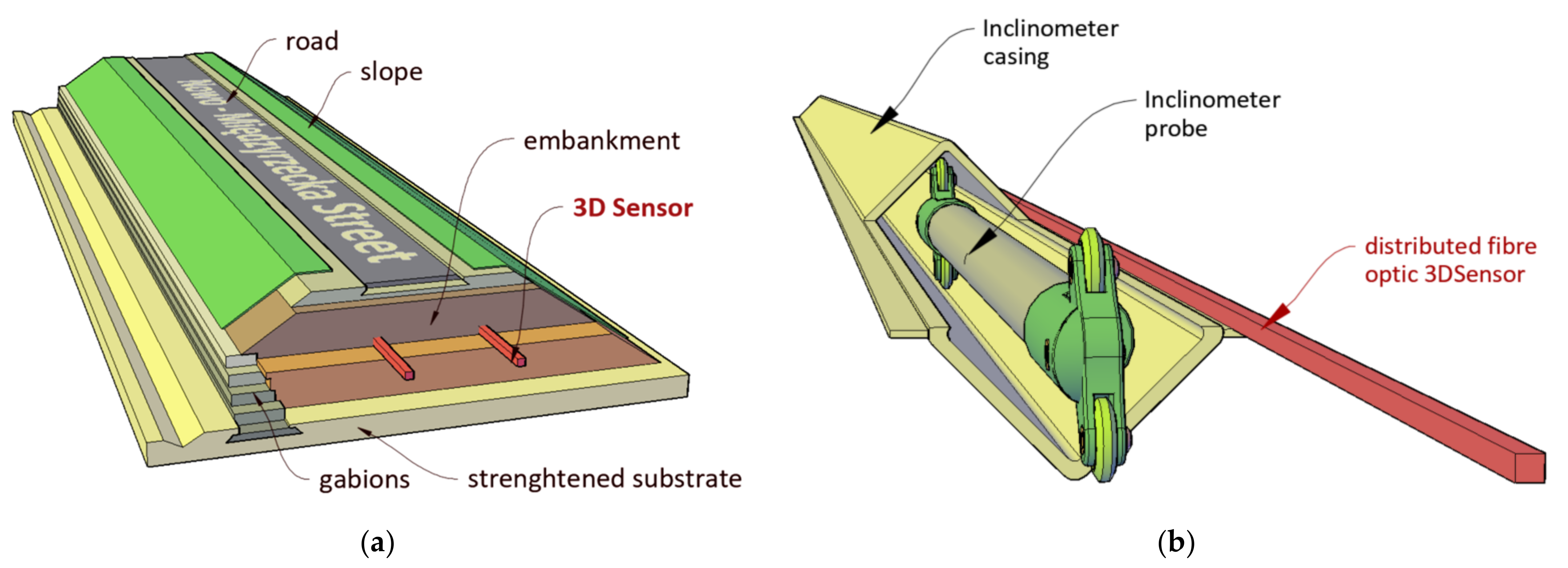
4. In Situ Application inside Embankment
4.1. General Description
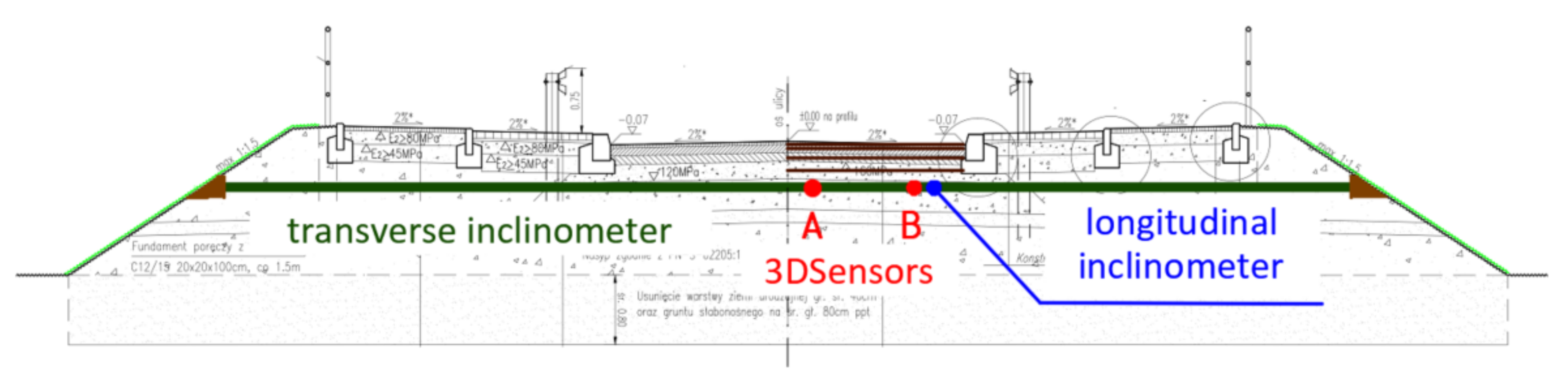
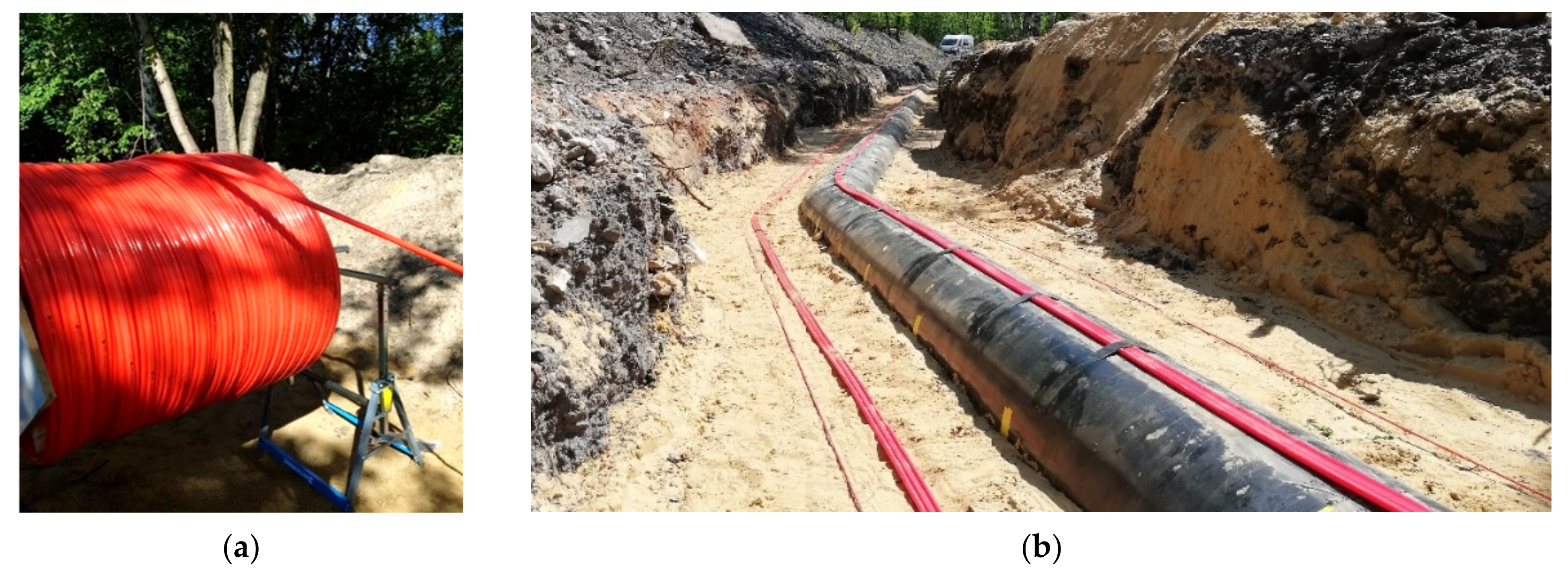
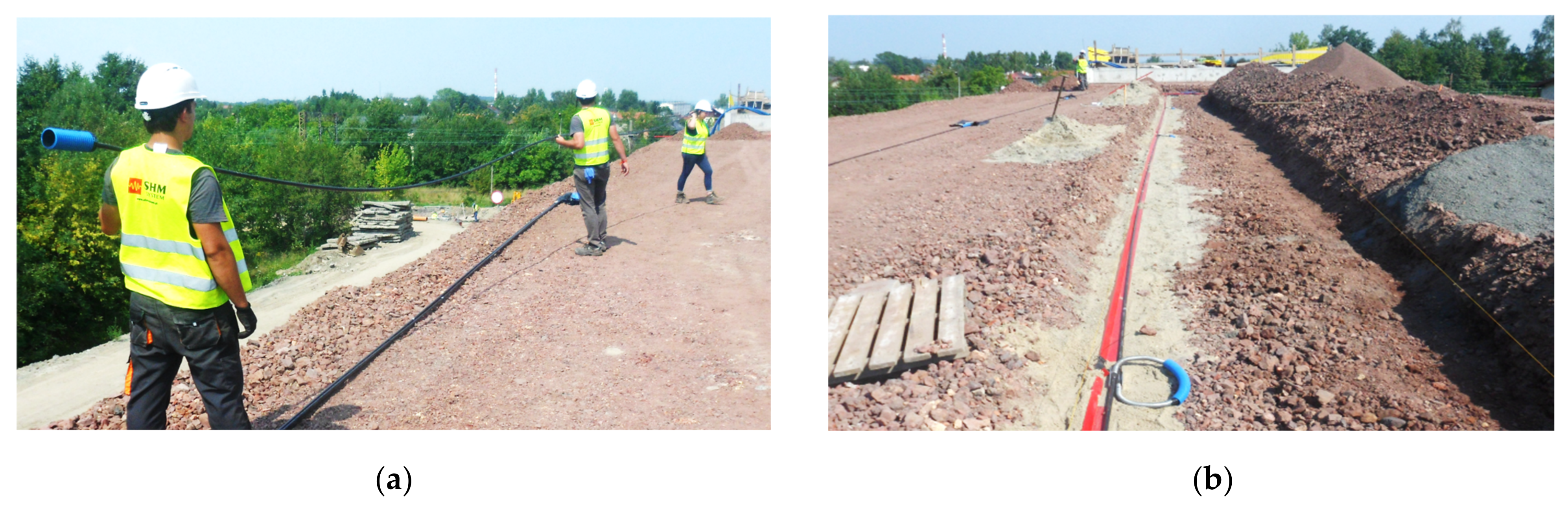
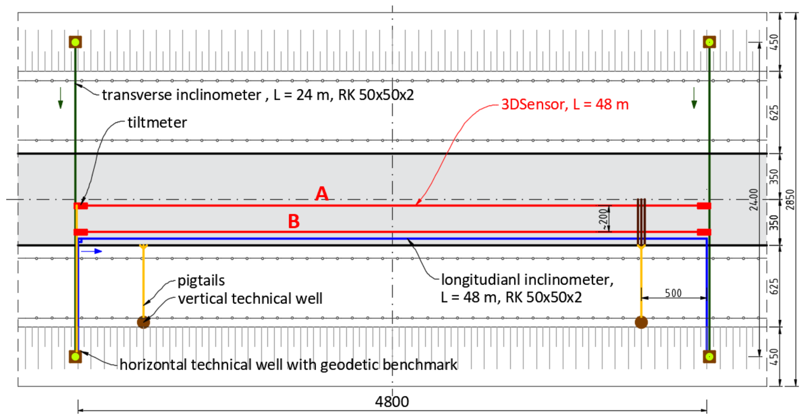
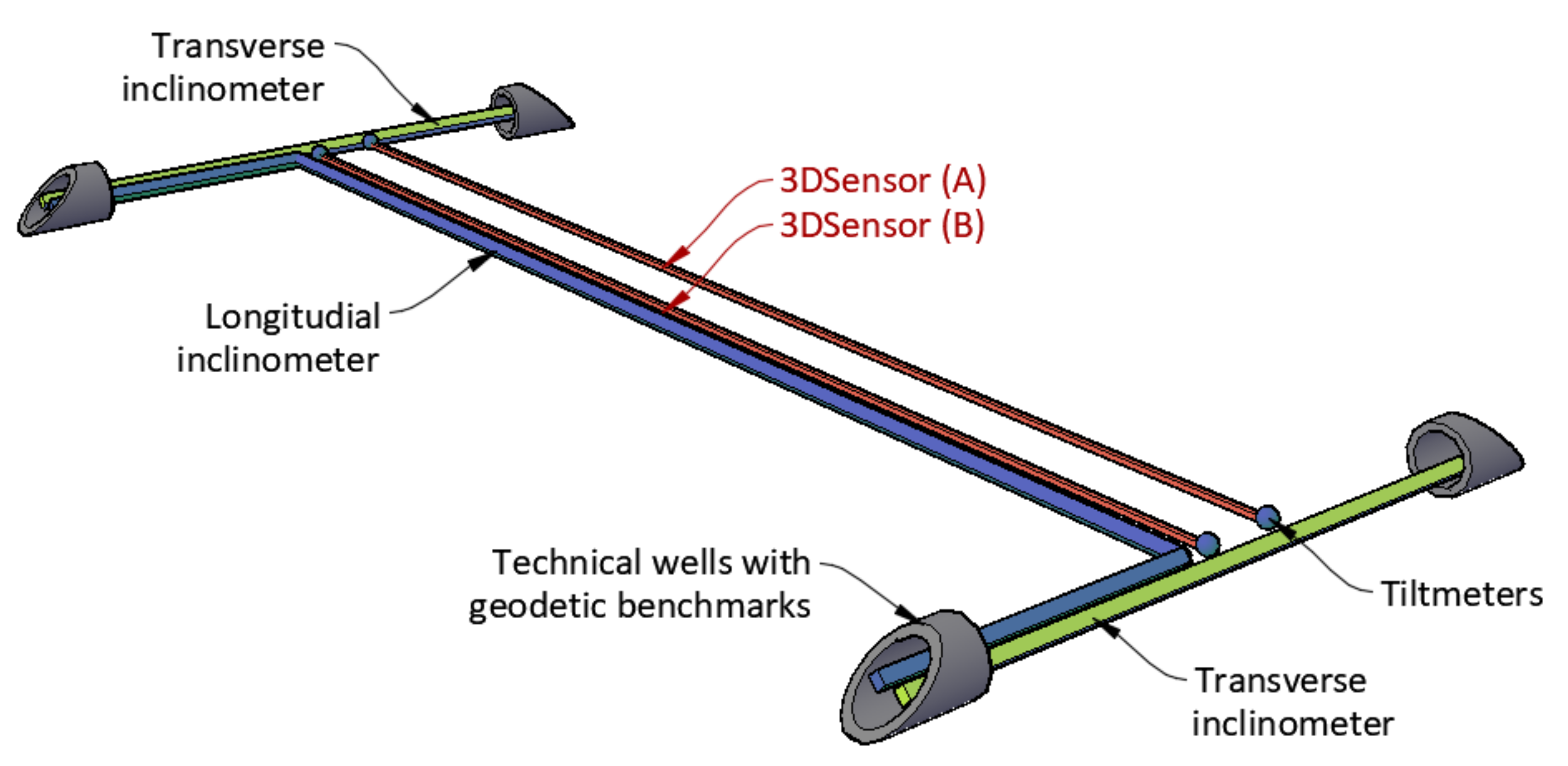
4.2. Sensors Delivery, Location and Installation
- Two transverse inclinometers;
- Four spot tiltmeters for rotations analysis at start and end points of the measuring lines;
- Geodetic benchmarks located in technical wells to analyse deformations in reference to the global coordinate system.
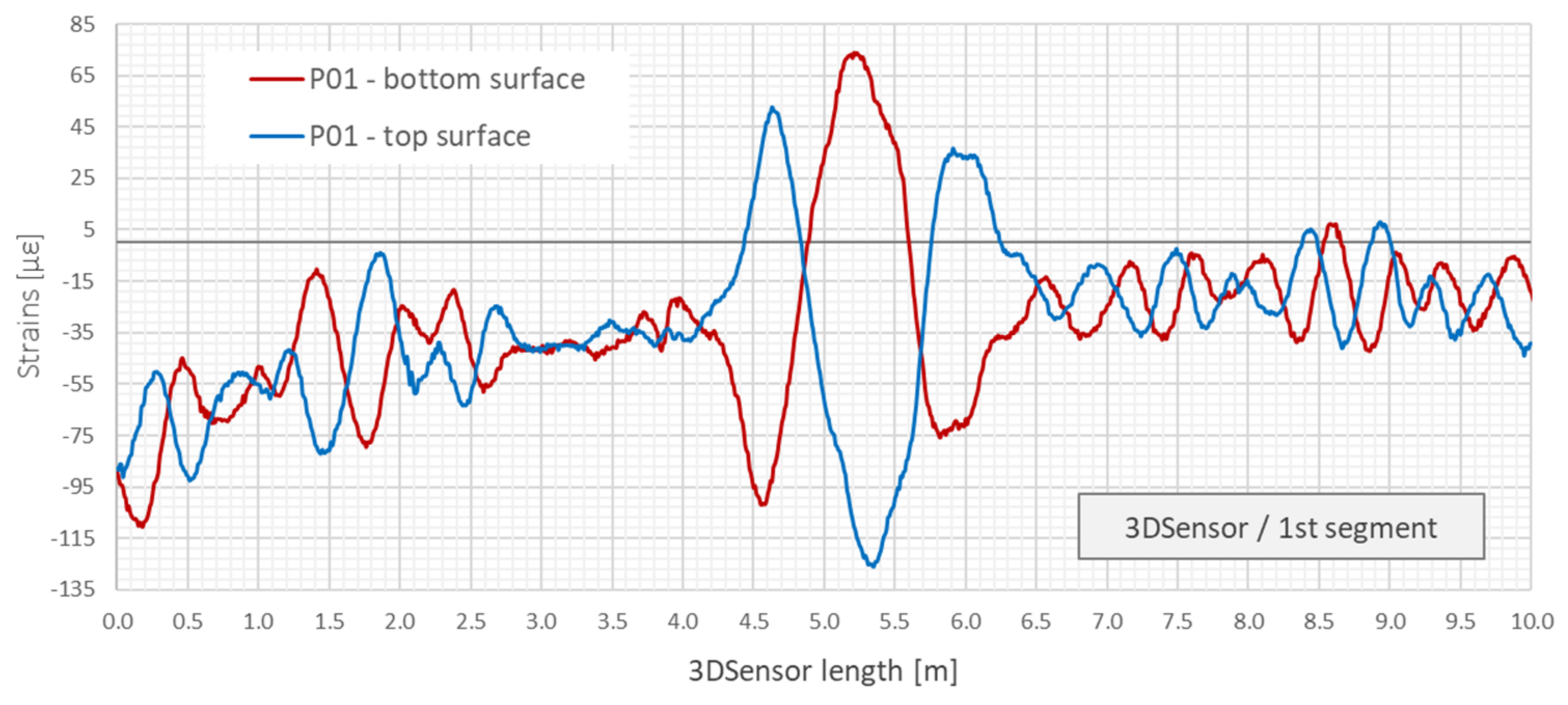
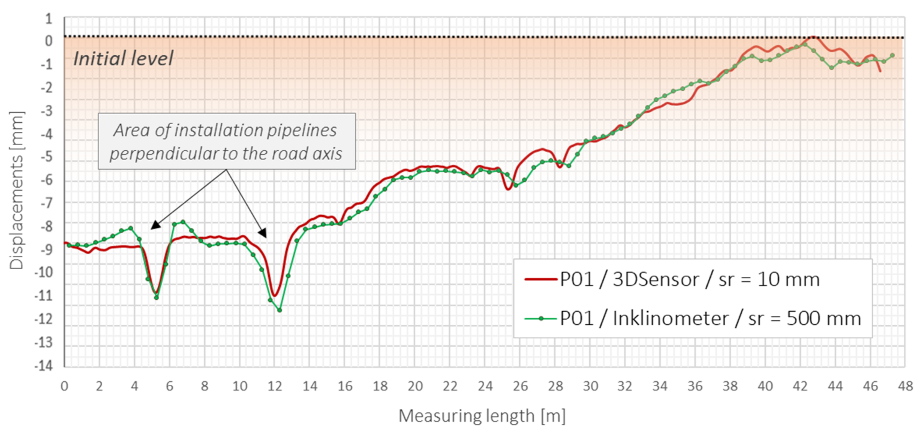
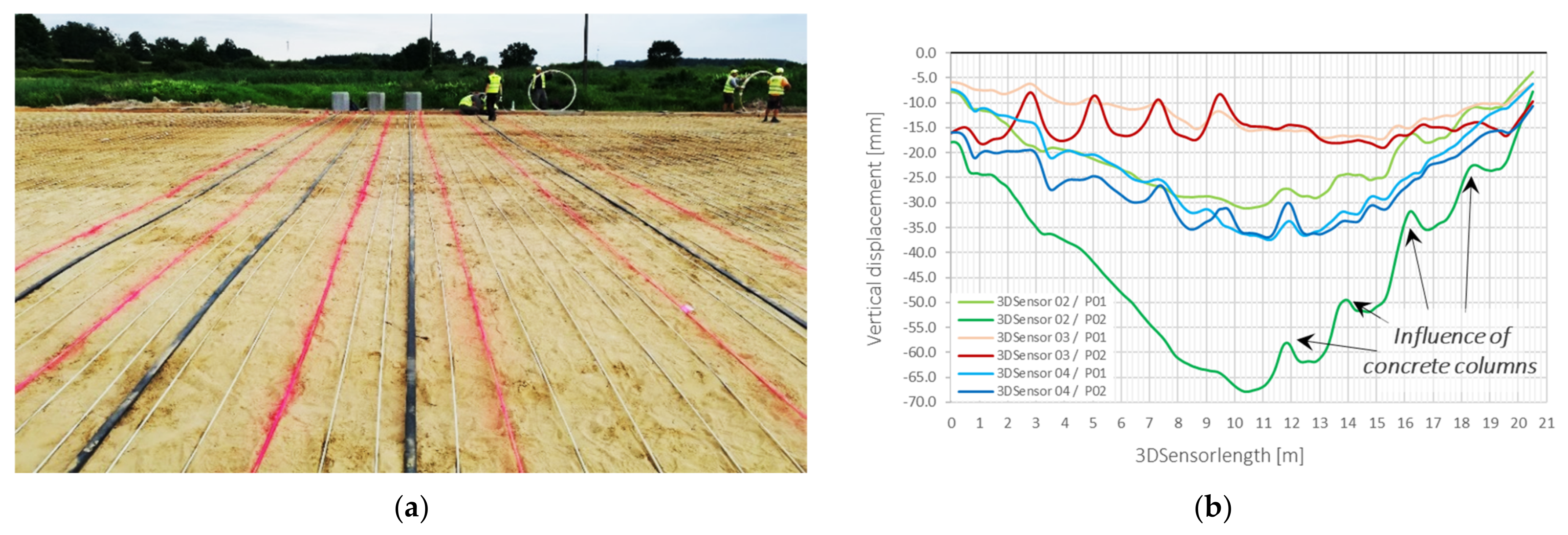
4.3. Example Results and Discussion
4.4. Another Proved Applications–Brief Review
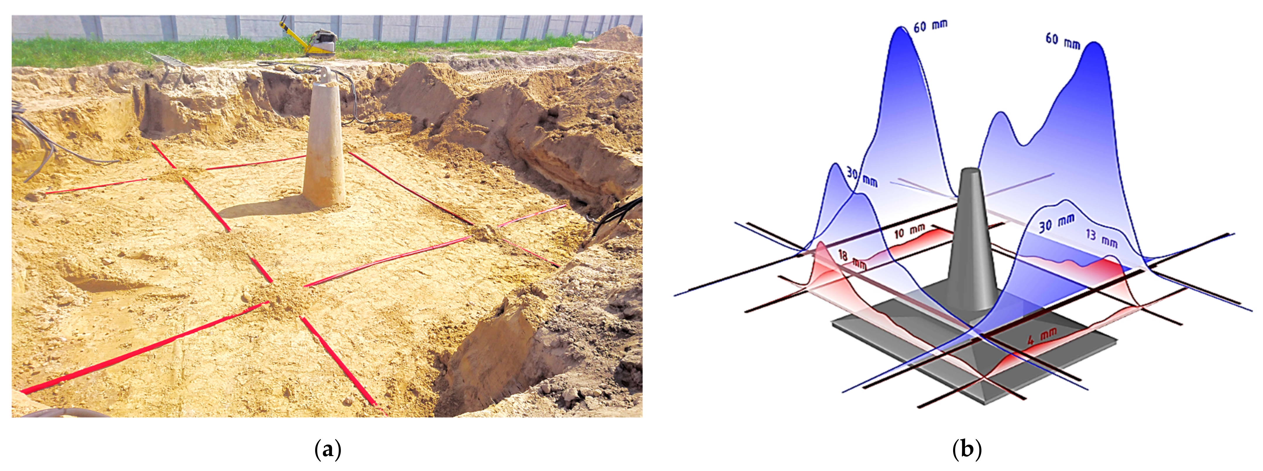
- Geotechnical research field [46], where different types of concrete footings design for electrical lines were pulled out from the ground for researching the shear plane. Figure 28a shows the installation process, while Figure 28b shows an example spatial visualization of displacement profiles obtained at a given load step;
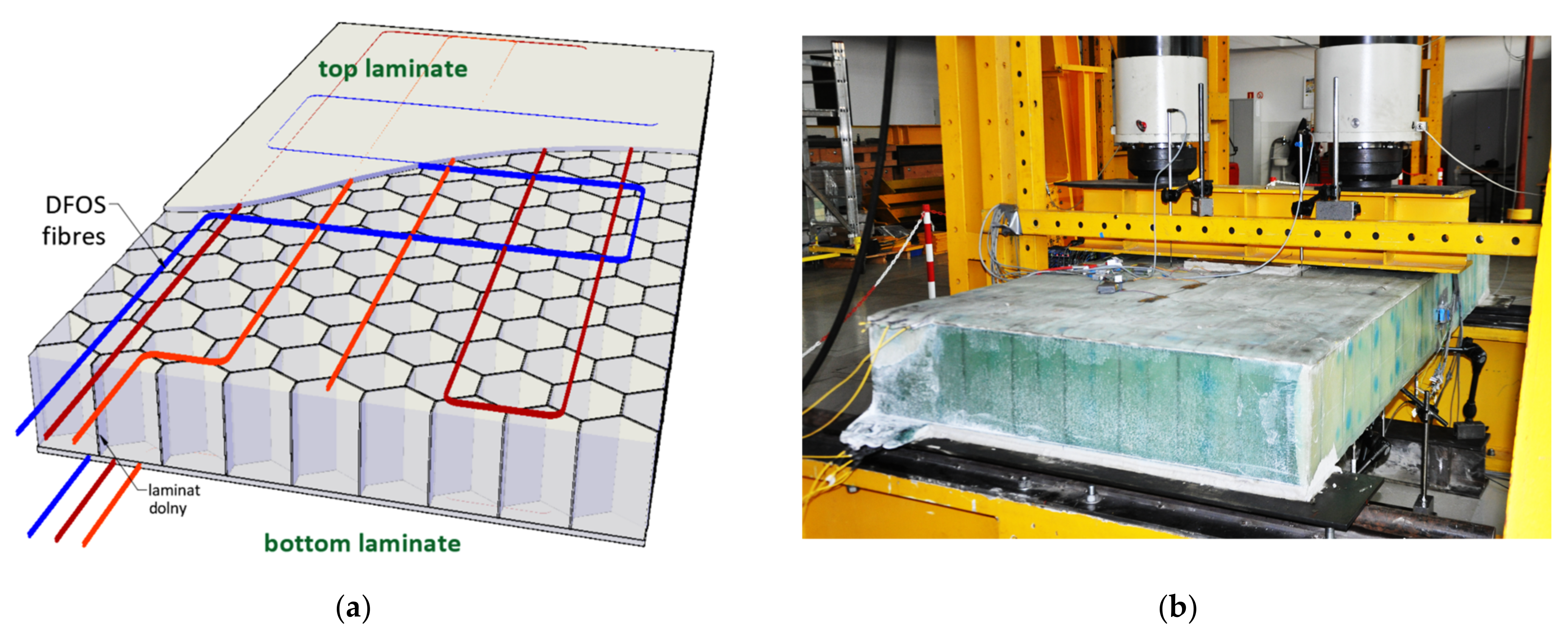
- Composite bridge panel [45], where during the infusion process, optical fibres were integrated with lower and upper laminates with the same idea as in the 3DSensor. Figure 31a shows the spatial visualization of designed panel, while in Figure 31b, the ready structure just before laboratory investigation is shown.
5. Conclusions
- Design of the sensor for measuring displacements in three directions (X, Y, Z);
- New application in geotechnics and civil engineering;
- Production technology (arrangement and integration of optical fibres within the sensor’s core during pultrusion);
- New composite material used as a sensor core.
6. Patents
Author Contributions
Funding
Institutional Review Board Statement
Informed Consent Statement
Data Availability Statement
Conflicts of Interest
References
- Faber, M.H. Statistics and Probability Theory in Pursuit of Engineering Decision Support; Springer: Dordrecht, The Netherlands; Heidelberg, Germany; London, UK; New York, NY, USA, 2012; ISBN 978-94-007-4055-6. [Google Scholar]
- Raiffa, H.; Schlaifer, R. Applied Statistical Decision Theory; Wiley: Hoboken, NJ, USA, 2000; ISBN 978-0-471-38349-9. [Google Scholar]
- Kishk, M.; Al-Hajj, A.; Pollock, R.; Bakis, N.; Aouad, G.F.; Bakis, N. Whole life costing in construction—A state of the art review. RICS Res. Paper Ser. 2003, 4. Available online: https://rgu-repository.worktribe.com/output/248559/whole-life-costing-in-construction-a-state-of-the-art-review (accessed on 25 May 2021).
- European Committee for Standardization CEN. EN 1990:2002 Eurocode 0: Basis of Structural Design; CEN: Brussels, Belgium, 2002. [Google Scholar]
- Balageas, D.; Fritzen, C.P.; Güemes, A. Structural Health Monitoring; Wiley-ISTE: Hoboken, NJ, USA, 2006; ISBN 978-1-905-20901-9. [Google Scholar]
- Xu, Y.L.; Xia, Y. Structural Health Monitoring of Long-Span Suspension Bridges; Spon Press: London, UK; New York, NY, USA, 2012; ISBN 9781138075634. [Google Scholar]
- Minardo, A.; Persichetti, G.; Testa, G.; Zeni, L.; Bernini, R. Long term structural health monitoring by Brillouin fibre-optic sensing: A real case. Smart Mater. Struct. 2012, 9, S64–S69. [Google Scholar] [CrossRef]
- Yuan, F.G. Structural Health Monitoring (SHM) in Aerospace Structures; Woodhead Publishing: Sawston, UK, 2016; ISBN 978-0-081-00158-5. [Google Scholar]
- Raffaella, D.S. Fibre Optic Sensors for Structural Health Monitoring of Aircraft Composite Structures: Recent Advances and Applications. Sensors 2015, 15, 18666–18713. [Google Scholar] [CrossRef]
- Guo, H.; Xiao, G.; Mrad, N.; Yao, J. Fiber Optic Sensors for Structural Health Monitoring of Air Platforms. Sensors 2011, 11, 3687–3705. [Google Scholar] [CrossRef]
- Sieńko, R.; Bednarski, Ł.; Howiacki, T. Smart Composite Rebars based on DFOS Technology as Nervous System of Hybrid Footbridge Deck: A Case Study. In Special Collection of 2020 Papers, Proceedings of the 8th European Workshop on Structural Health Monitoring, Palermo, Italy, 6–9 July 2021; Springer: Berlin/Heidelberg, Germany, 2021; Volume 2, pp. 340–350. ISBN 978-3-030-64908-1. [Google Scholar]
- Zhou, G.; Sim, L.M. Damage detection and assessment in fibre-reinforced composite structures with embedded fibre optic sensors-review. Smart Mater. Struct. 2002, 11, 925–939. [Google Scholar] [CrossRef]
- Soga, K.; Luo, L. Distributed fiber optics sensors for civil engineering infrastructure sensing. J. Struct. Integr. Maint. 2018, 3, 1–21. [Google Scholar] [CrossRef]
- Cheng-Yu, H.; Yi-Fan, Z.; Guo-Wei, L.; Meng-Xi, Z.; Zi-Xiong, L. Recent progress of using Brillouin distributed fiber sensors for geotechnical health monitoring. Sens. Actuators A Phys. 2017, 258, 131–145. [Google Scholar] [CrossRef]
- Dibiago, E. A Case study of Vibrating-Wire Sensors That Have Vibrated Continuously for 27 Years. In Field Measurements in Geomechanics, Proceedings of the 6th International Symposium, Oslo, Norway, 23–26 September 2003; A. A. Balkema: Rotterdam, The Netherlands, 2003; pp. 445–458. [Google Scholar]
- Cieplok, G.; Bednarski, Ł. Measurements of Dynamic Deformations of Building Structures by Applying Wire Sensors. Sensors 2019, 19, 255. [Google Scholar] [CrossRef] [Green Version]
- Lin, Y.B.; Chang, K.; Chern, J.C.; Wang, A.L. The health monitoring of a prestressed concrete beam by using fiber Bragg grating sensors. Smart Mater. Struct. 2004, 13, 712–718. [Google Scholar] [CrossRef] [Green Version]
- Howiacki, T.; Sieńko, R.; Sýkora, M. Reliability analysis of serviceability of long span roof using measurements and FEM model. AIP Conf. Proc. 2019, 2116, 450078. [Google Scholar] [CrossRef]
- Barrias, A.; Casas, J.R.; Villaba, S. Application study of embedded Rayleigh based Distributed Optical Fiber Sensors in concrete beams. Procedia Eng. 2017, 199, 2014–2019. [Google Scholar] [CrossRef] [Green Version]
- Barrias, A.; Casas, J.R.; Villalba, S. Embedded Distributed Optical Fiber Sensors in Reinforced Concrete Structures—A Case Study. Sensors 2018, 18, 980. [Google Scholar] [CrossRef] [PubMed] [Green Version]
- Wang, H.; Xiang, P. Strain transfer analysis of optical fiber-based sensors embedded in an asphalt pavement structure. Meas. Sci. Technol. 2016, 27, 075106. [Google Scholar] [CrossRef]
- European Committee for Standardization CEN. EN 1997-1:2004, Eurocode 7: Geotechnical Design—Part 1: General Rules; CEN: Brussels, Belgium, 2004. [Google Scholar]
- Zhou, D.P.; Li, W.; Chen, L.; Bao, X. Distributed Temperature and Strain Discrimination with Stimulated Brillouin Scattering and Rayleigh Backscatter in an Optical Fiber. Sensors 2013, 13, 1836–1845. [Google Scholar] [CrossRef] [PubMed] [Green Version]
- Liu, T.; Huang, H.; Yang, Y. Crack Detection of Reinforced Concrete Member Using Rayleigh-Based Distributed Optic Fiber Strain Sensing System. Adv. Civ. Eng. 2020, 2020, 8312487. [Google Scholar] [CrossRef]
- Bao, X.; Chen, L. Recent Progress in Brillouin Scattering Based Fiber Sensors. Sensors 2011, 11, 4152–4187. [Google Scholar] [CrossRef] [PubMed]
- Imai, M.; Feng, M. Sensing optical fiber installation study for crack identification using a stimulated Brillouin-based strain sensor. Struct. Health Monit. 2012, 11, 501–509. [Google Scholar] [CrossRef]
- Nöther, N.; Facchini, M. Distributed fiber-optic strain sensing: Field applications in pile foundations and concrete beams. In Proceedings of the 8th Civil Structural Health Monitoring Workshop (CSHM-8), Naples, Italy, 29–31 March 2021. [Google Scholar]
- Liu, Y.; Li, X.; Li, H.; Fan, X. Global Temperature Sensing for an Operating Transformer Based on Raman Scattering. Sensors 2020, 20, 4903. [Google Scholar] [CrossRef]
- Samiec, D. 2012. Distributed fibre-optic temperature and strain measurement with extremely high spatial resolution. Photonic Int. 2012, 6, 10–13. [Google Scholar]
- Sang, A.K.; Froggatt, M.E.; Kreger, S.T.; Gifford, D.K. Millimeter resolution distributed dynamic strain measurements using optical frequency domain reflectometry. In Proceedings of the 21st International Conference on Optical Fiber Sensors, Ottawa, ON, Canada, 15–19 May 2011; Volume 7753, p. 77532S. [Google Scholar] [CrossRef]
- Bassil, A.; Wang, X.; Chapeleau, X.; Niederleithinger, E. Distributed fiber optics sensing and coda wave interferometry techniques for damage monitoring in concrete structures. Sensors 2019, 19, 356. [Google Scholar] [CrossRef] [Green Version]
- Sieńko, R.; Zych, M.; Bednarski, Ł.; Howiacki, T. Strain and crack analysis within concrete members using distributed fibre optic sensors. Struct. Health Monit. 2018, 18, 1510–1526. [Google Scholar] [CrossRef]
- Funnel, A.; Xu, X.; Yan, J.; Soga, K. Simulation of Noise within BOTDA and COTDR Systems to Study the Impact on Dynamic Sensing. Int. J. Smart Sens. Intell. Syst. 2015, 8, 1576–1600. [Google Scholar] [CrossRef] [Green Version]
- Weisbrich, M.; Holschemacher, K. Comparison between different fiber coatings and adhesives on steel surfaces for distributed optical strain measurements based on Rayleigh backscattering. J. Sens. Sens. Syst. 2018, 7, 601–608. [Google Scholar] [CrossRef] [Green Version]
- Li, Q.; Li, G.; Wang, G. Effect of the plastic coating on strain measurement of concrete by fiber optic sensor. Measurement 2003, 34, 215–227. [Google Scholar] [CrossRef]
- Barrias, A.; Casas, J.R.; Villalba, S. A Review of Distributed Optical Fiber Sensors for Civil Engineering Applications. Sensors 2016, 16, 748. [Google Scholar] [CrossRef] [Green Version]
- Sieńko, R.; Bednarski, Ł.; Howiacki, T. Application of Distributed Optical Fibre Sensor for Strain and Temperature Monitoring within Continuous Flight Auger Columns. In Proceedings of the 4th World Multidisciplinary Earth Sciences Symposium WMESS, Prague, Czech Republic, 3–7 September 2018. [Google Scholar]
- Li, Q.; Li, G.; Wang, G.; Ansari, F.; Asce, M.; Liu, Q. Elasto-Plastic Bonding of Embedded Optical Fiber Sensors in Concrete. J. Eng. Mech. 2002, 128. [Google Scholar] [CrossRef]
- Lally, E.M.; Reaves, M.; Horrell, E.; Klute, S.; Froggatt, M.E. Fiber optic shape sensing for monitoring of flexible structures. In Proceedings of the SPIE 8345, Sensors and Smart Structures Technologies for Civil, Mechanical, and Aerospace Systems, San Diego, CA, USA, 11–15 March 2012; p. 83452Y. [Google Scholar] [CrossRef]
- Amanzadehab, M.; Aminossadatia, S.M.; Kizil, M.S.; Rakićb, A.D. Recent developments in fibre optic shape sensing. Measurement 2018, 128, 119–137. [Google Scholar] [CrossRef] [Green Version]
- Kishida, K.; Yamauchi, Y.; Nishiguchi, K.; Guzik, A. Monitoring of tunnel shape using distributed optical fiber sensing techniques. In Proceedings of the 4th Conference on Smart Monitoring, Assessment and Rehabilitation of Civil Structures SMAR 2017, Zurich, Switzerland, 13–15 September 2017. [Google Scholar]
- Schenato, L. A Review of Distributed Fibre Optic Sensors for Geo-Hydrological Applications. Appl. Sci. 2017, 7, 896. [Google Scholar] [CrossRef]
- Sun, Y.; Shi, B.; Zhang, D.; Tong, H.; Wei, G.; Xu, H. Internal Deformation Monitoring of Slope Based on BOTDR. J. Sens. 2016, 2016, 9496285. [Google Scholar] [CrossRef]
- Huang, X.; Wang, Y.; Sun, Y.; Zhang, Q.; Zhang, Z.; You, Z.; Ma, Y. Research on horizontal displacement monitoring of deep soil based on a distributed optical fibre sensor. J. Mod. Opt. 2017, 65, 158–165. [Google Scholar] [CrossRef]
- Kulpa, M.; Howiacki, T.; Wiater, A.; Siwowski, T.; Sieńko, R. Strain and displacement measurement based on distributed fibre optic sensing (DFOS) system integrated with FRP composite sandwich panel. Measurement 2021, 175, 109099. [Google Scholar] [CrossRef]
- Sieńko, R.; Bednarski, Ł.; Howiacki, T.; Zuziak, K.; Labocha, S. Possibilities of composite distributed fibre optic 3DSensor on the example of footing pulled out from the ground: A case study. In Proceedings of the 8th Civil Structural Health Monitoring Workshop (CSHM-8), Naples, Italy, 29–31 March 2021. [Google Scholar]
- Vedernikov, A.; Safonov, A.; Tucci, F.; Carlone, P.; Akhatov, I. Pultruded materials and structures: A review. J. Compos. Mater. 2020, 54, 4081–4117. [Google Scholar] [CrossRef]
- Luna Innovations. Optical Backscatter Reflectometer—Model 4600. User Guide 6, OBR 4600 Software 3.10.1; Luna Technologies: Roanoke, VA, USA, 2013. [Google Scholar]
- Allasia, P.; Godone, D.; Giordan, D.; Guenzi, D.; Lollino, G. Advances on Measuring Deep-Seated Ground Deformations Using Robotized Inclinometer System. Sensors 2020, 20, 3769. [Google Scholar] [CrossRef] [PubMed]
- Ruzza, G.; Guerriero, L.; Revellino, P.; Guadagno, F.M. A Multi-Module Fixed Inclinometer for Continuous Monitoring of Landslides: Design, Development, and Laboratory Testing. Sensors 2020, 20, 3318. [Google Scholar] [CrossRef] [PubMed]
- Bednarski, Ł.; Milewski, S.; Sieńko, R. Determination of vertical and horizontal soil displacements in automated measuring systems on the basis of angular measurements. Tech. Trans. 2014, 6-B, 3–13. Available online: http://suw.biblos.pk.edu.pl/resources/i5/i1/i6/i6/i1/r51661/BednarskiL_DeterminationVertical.pdf (accessed on 25 May 2021).
- INCLIFY—Automated Monitoring System. Available online: https://inclify.com/en (accessed on 25 May 2021).
- NERVE Composite DFOS Sensors. Available online: http://nerve-sensors.com (accessed on 25 May 2021).
- SHM System. Available online: http://www.shmsystem.pl (accessed on 25 May 2021).


| No. | Issue | Work Description | Solution/Result |
|---|---|---|---|
| 1 | Selection and calibration of optical fibre and its primary coating. | Statistical laboratory research on selected optical fibres with different types of primary coatings (acrylate, polyimide, experimental sand-grained). | Selection of the standard telecom SM9/125 optical fibre in soft acrylate coating. |
| 2 | Analysis of the influence of additional (secondary) coatings. | Statistical laboratory research on selected types of secondary coatings, including tight jackets. | Removal of all additional fibre coatings. |
| 3 | Selection of the material for sensor’s core ensuring high elastic range. | Statistical laboratory research on selected materials (steel, plastics, rubbers, composites). | Composite core with elastic strain range up to ±4%. |
| 4 | Integration method of the fibres and sensor’s core. | Research on different types of adhesives and other technological possibilities. | Integration of the fibres at production (pultrusion) stage. |
| 5 | Algorithms for data processing. | Theoretical studies including state-of-the-art review, analytical work and numerical simulations. | 4 algorithms for displacement calculations: beam deflection equation, explicit methods of the first and the second order, trapezoidal method. |
| 6 | Thermal compensation. | Laboratory research on thermal compensation systems effectiveness. | Additional compensating fibre, thermal self-compensation system. |
| 7 | Accuracy of displacements. | Statistical laboratory research on different versions of the sensor with reference techniques. | Data sheet including technical specifications. |
| 8 | Repeatability and long-term stability. | Statistical laboratory research over long term. | Data sheet including technical specifications. |
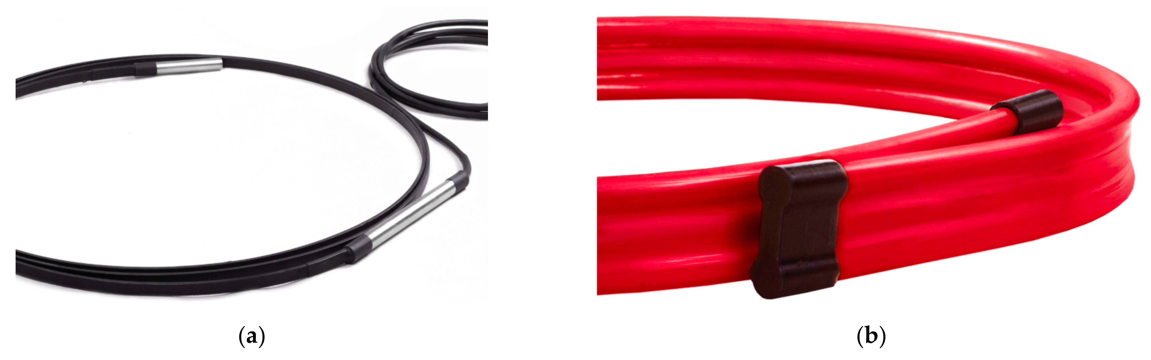
| 9 | Connection of the sensor’s segments. | Laboratory research on different types of connections and protective casings. | Design of the way to connect the sensor in case of breakage. |
| 10 | Wide range of proven field applications. | Sensors’ demonstration installations in field conditions (2 x bridge, 1 x industrial tower, 5 x geotechnical structures, inc. slurry walls and embankments, others). | Installation, measurements, data processing, real performance → lessons learned (see also Section 4). |
| Parameter | Value | Unit |
|---|---|---|
| Measurement length (standard mode) | 70 | m |
| Spatial resolution (gauge spacing) 1 | 10 | mm |
| Gauge length 2 | 10 | mm |
| Strain measurement resolution | ±1.0 | mm |
| No. | Vertical Displacements | Horizontal Shortenings over x Axis | ||||||
|---|---|---|---|---|---|---|---|---|
| dz,ref (mm) | dz,3D (mm) | eabsolute (mm) | erelative (%) | dz,FEA (mm) | dx,3DS (mm) | eabsolute (mm) | erelative (%) | |
| P01 | 3.000 | 2.994 | 0.006 | 0.196 | 0.013 | 0.013 | 0.000 | 1.831 |
| P02 | 6.001 | 6.017 | −0.016 | −0.268 | 0.054 | 0.051 | 0.003 | 4.696 |
| P03 | 9.000 | 9.019 | −0.019 | −0.208 | 0.121 | 0.116 | 0.005 | 4.461 |
| P04 | 12.001 | 12.049 | −0.048 | −0.397 | 0.214 | 0.206 | 0.008 | 3.648 |
| P05 | 15.000 | 15.054 | −0.054 | −0.362 | 0.335 | 0.322 | 0.013 | 3.962 |
| P06 | 17.999 | 18.069 | −0.070 | −0.387 | 0.482 | 0.463 | 0.019 | 3.899 |
| P07 | 21.000 | 21.084 | −0.084 | −0.401 | 0.656 | 0.631 | 0.025 | 3.880 |
| P08 | 23.999 | 24.078 | −0.079 | −0.330 | 0.857 | 0.822 | 0.035 | 4.071 |
| P09 | 27.001 | 27.037 | −0.036 | −0.133 | 1.085 | 1.033 | 0.052 | 4.779 |
| P10 | 30.000 | 30.218 | −0.218 | −0.727 | 1.339 | 1.290 | 0.049 | 3.677 |
| P11 | 33.000 | 33.159 | −0.159 | −0.483 | 1.620 | 1.555 | 0.065 | 4.040 |
| P12 | 36.001 | 36.108 | −0.107 | −0.296 | 1.928 | 1.844 | 0.084 | 4.342 |
| P13 | 39.000 | 39.101 | −0.101 | −0.258 | 2.263 | 2.164 | 0.099 | 4.396 |
| P14 | 42.002 | 42.376 | −0.374 | −0.891 | 2.624 | 2.535 | 0.089 | 3.390 |
| P15 | 39.001 | 38.953 | 0.048 | 0.123 | 2.263 | 2.142 | 0.121 | 5.328 |
| P16 | 36.001 | 36.021 | −0.020 | −0.055 | 1.928 | 1.829 | 0.099 | 5.122 |
| P17 | 33.001 | 33.050 | −0.049 | −0.148 | 1.62 | 1.538 | 0.082 | 5.059 |
| P18 | 30.001 | 30.055 | −0.054 | −0.181 | 1.339 | 1.270 | 0.069 | 5.137 |
| P19 | 27.000 | 27.078 | −0.078 | −0.289 | 1.085 | 1.029 | 0.056 | 5.117 |
| P20 | 24.000 | 24.084 | −0.084 | −0.348 | 0.857 | 0.813 | 0.044 | 5.125 |
| P21 | 21.000 | 21.071 | −0.071 | −0.337 | 0.656 | 0.621 | 0.035 | 5.286 |
| P22 | 18.000 | 18.079 | −0.079 | −0.438 | 0.482 | 0.456 | 0.026 | 5.358 |
| P23 | 15.000 | 15.070 | −0.070 | −0.464 | 0.335 | 0.316 | 0.019 | 5.571 |
| P24 | 12.000 | 12.064 | −0.064 | −0.535 | 0.214 | 0.202 | 0.012 | 5.715 |
| P25 | 9.000 | 9.062 | −0.062 | −0.687 | 0.121 | 0.113 | 0.008 | 6.530 |
| P26 | 6.001 | 6.069 | −0.068 | −1.133 | 0.054 | 0.050 | 0.004 | 7.374 |
| P27 | 3.001 | 3.063 | −0.062 | −2.080 | 0.013 | 0.012 | 0.001 | 5.292 |
| Mean: | −0.077 | −0.427 | Mean: | 0.042 | 4.707 | |||
| Stdv 1: | 0.076 | 0.424 | Stdv 1: | 0.035 | 1.049 | |||
| Parameter | Value |
|---|---|
| Displacement range | ±250 mm/m |
| Displacement resolution | ±3 mm/30 m |
| Displacement resolution | ±0.02 mm/m |
| Spatial resolution | 500–1000 mm |
| Type of the probe | MEMS |
| Operation temperature | from −40 °C to +85 °C |
| Parameter | Value |
|---|---|
| Displacement range | any, dependent on static scheme |
| Displacement resolution | ±1 mm |
| Operation temperature | from −20 °C to +60 °C |
| Standard dimensions of active core 1 | 8 × 6 mm |
| Standard external dimensions 1 | 50 × 15 mm |
| Sensor material | PLFRP + PE |
| Light scattering 2 | Rayleigh, Brillouin, Raman |
| Delivery method | coils or straight sections |
| Length | any length made to order |
Publisher’s Note: MDPI stays neutral with regard to jurisdictional claims in published maps and institutional affiliations. |
© 2021 by the authors. Licensee MDPI, Basel, Switzerland. This article is an open access article distributed under the terms and conditions of the Creative Commons Attribution (CC BY) license (https://creativecommons.org/licenses/by/4.0/).
Share and Cite
Bednarski, Ł.; Sieńko, R.; Grygierek, M.; Howiacki, T. New Distributed Fibre Optic 3DSensor with Thermal Self-Compensation System: Design, Research and Field Proof Application Inside Geotechnical Structure. Sensors 2021, 21, 5089. https://doi.org/10.3390/s21155089
Bednarski Ł, Sieńko R, Grygierek M, Howiacki T. New Distributed Fibre Optic 3DSensor with Thermal Self-Compensation System: Design, Research and Field Proof Application Inside Geotechnical Structure. Sensors. 2021; 21(15):5089. https://doi.org/10.3390/s21155089
Chicago/Turabian StyleBednarski, Łukasz, Rafał Sieńko, Marcin Grygierek, and Tomasz Howiacki. 2021. "New Distributed Fibre Optic 3DSensor with Thermal Self-Compensation System: Design, Research and Field Proof Application Inside Geotechnical Structure" Sensors 21, no. 15: 5089. https://doi.org/10.3390/s21155089
APA StyleBednarski, Ł., Sieńko, R., Grygierek, M., & Howiacki, T. (2021). New Distributed Fibre Optic 3DSensor with Thermal Self-Compensation System: Design, Research and Field Proof Application Inside Geotechnical Structure. Sensors, 21(15), 5089. https://doi.org/10.3390/s21155089