
Privacy-Preserving Energy Management of a Shared Energy Storage System for Smart Buildings: A Federated Deep Reinforcement Learning Approach


Abstract
:1. Introduction
- We present a distributed FRL architecture in which the energy consumption of smart buildings and the energy charging and discharging of the SESS are optimally scheduled within the heterogeneous environments of the buildings while preserving the privacy of energy usage information of individual buildings.
- We develop a robust privacy-preserving FRL-based BEMS algorithm against building privacy leakage in the hierarchically distributed architecture. During the FRL process, the HVAC DRL agent improves the energy consumption model of the LBEMS through an iterative interaction with the GS and preserves the privacy of energy usage data using a selective parameter sharing method. Subsequently, the SESS DRL agent trains the optimal energy charging and discharging model of the SESS by using the LBEMS agent’s neural network model without sharing the relevant energy consumption data to preserve the privacy of the buildings’ energy consumption.
2. Background of Reinforcement Learning
2.1. Markov Decision Process (MDP)
2.2. Deep Reinforcement Learning
2.3. Federated Reinforcement Learning
3. Energy Management of a Shared ESS for Smart Buildings Using FRL
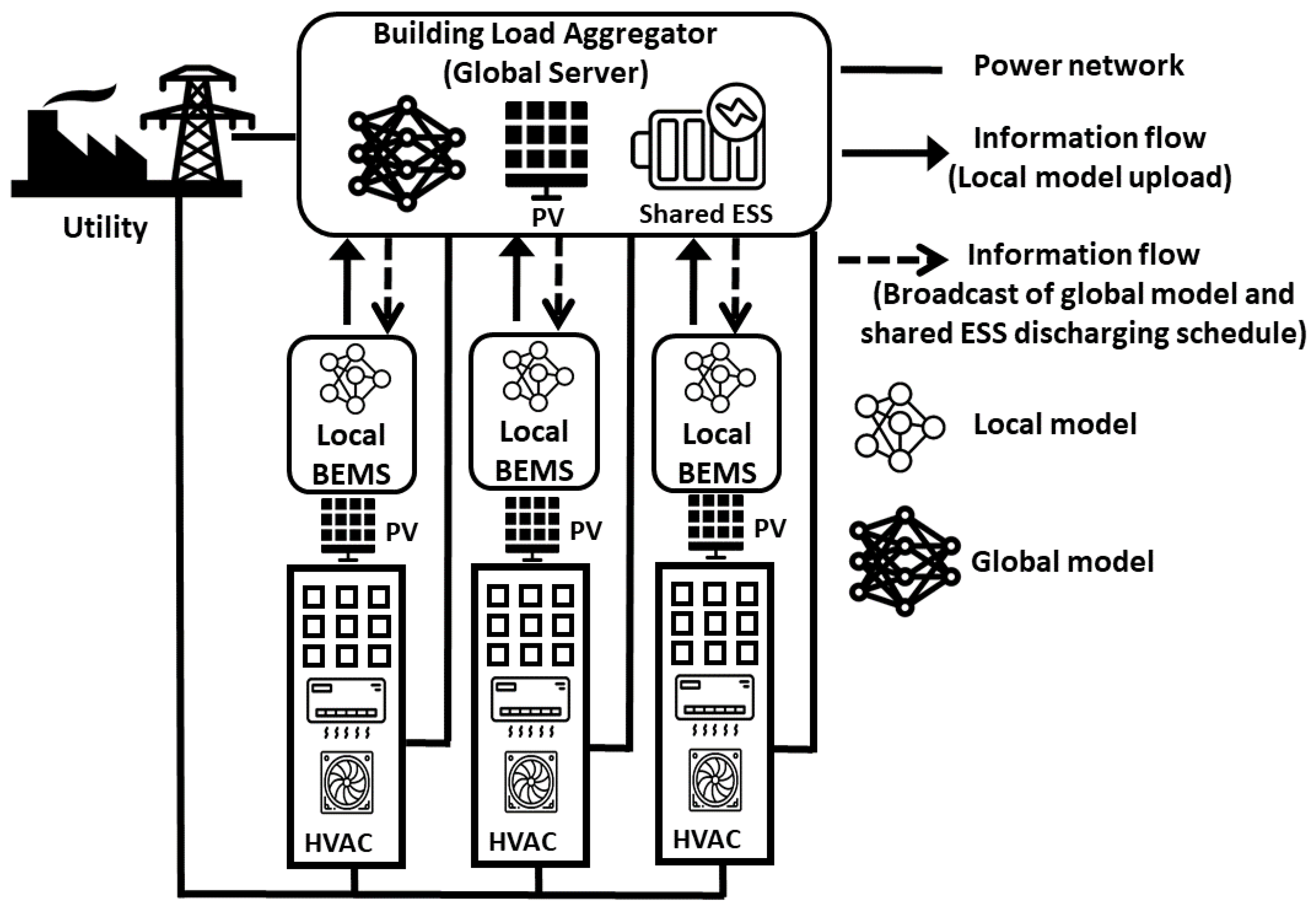
3.1. System Configuration
- Step (1) FRL for HVAC energy consumption scheduling: each HVAC agent in the LBEMS trains its own model to schedule the energy consumption of HVAC using the actor–critic method with its data. The randomly selected part of trained local models (i.e., the weights of its local neural network for LBEMS n) are periodically transmitted to the GS. Subsequently, the GS aggregates and updates the global model (i.e., the weights of the global neural network) using the federated stochastic gradient descent (FedSGD) algorithm [30] that averages the local models (). The updated global model is distributed to all LBEMSs where all HVAC agents update their own models based on the global model. The updated local models and global model are exchanged iteratively until a predetermined stopping criterion is satisfied.
- Step (2) SESS charging/discharging: the optimal HVAC energy consumption models calculated from Step (1) along with the fixed loads in the building are fed back into the GS where the SESS agent trains the model for charging and discharging energy from and to the utility and the LBEMSs using the actor–critic method. The trained discharging schedules are transmitted to the LBEMSs, and these schedules are added to the HVAC energy consumption schedules that are calculated by the HVAC agents in Step (1).
3.2. System Description for HVAC and SESS Agents
3.2.1. State Space
3.2.2. Action Space
3.2.3. Reward Function
3.3. Proposed Privacy-Preserving Energy Management of the SESS with Smart Buildings
- Prior to the learning procedure, the energy consumptions and discomfort parameters of both HVAC and SESS agent are initialized (line 1).
- Probability of actions, weights of the actor network and the critic network, Q-value for the HVAC and the SESS agent are initialized (line 2).
- The global neural network model in the GS along with the sharing batch for the FRL approach is initialized (line 3).
- During every local training episode per communication round, each building’s HVAC agent iterates the following procedures to compute its optimal energy consumption schedule from to (line 6∼13).
- (a)
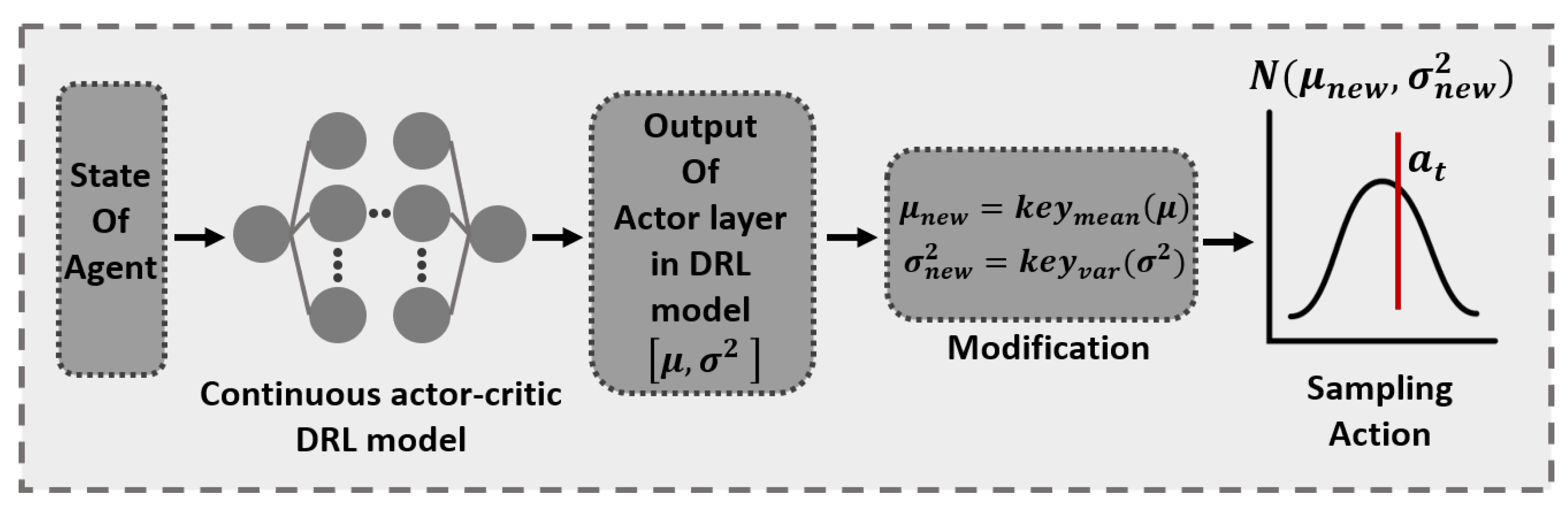
- Sample action based on distribution generated by actor network and key functions in state (line 8).
- (b)
- Execute action , receive reward from the action and from the critic network, and finally, calculate the target value of critic network, (line 9).
- (c)
- Compute the loss functions of actor network and critic network to minimize the losses and update the model of the HVAC agent using the ADAM optimizer [39] (lines 10, 11).
- The HVAC agent n randomly selects a part of its local model from the fully trained model and transmit it to the GS where it is stored in batch (lines 14, 15).
- The GS yields a global neural network model by executing the FedSGD method with the selected weights in (line 17).
- This newly generated global model is distributed to all HVAC agents in LBEMSs where those agents resume their own training based on (lines 18, 19).
- All HVAC agents transmit their fully trained model to the GS (line 21).
- For training episodes, the SESS agent repeats the following procedures to search for an optimal charging and discharging schedule from to (line 23∼31).
- (a)
- The SESS agent infers the energy consumption of the LBEMS n using the model and the state (line 25).
- (b)
- Sample an action based on distribution generated by the actor network and the key functions given by state , which includes the inferred energy consumption data for all LBEMSs (line 26).
- (c)
- Compute action , receive reward and from the critic network, and calculate of the SESS agent (line 27).
- (d)
- Estimate the loss functions of the actor network and the critic network by minimizing them, and update the model of the SESS agent using the ADAM optimizer (line 28, 29).
| Algorithm 1: FRL-based energy management of a SESS with multiple smart buildings. |
 |
4. Simulation Results
4.1. Simulation Setup
4.2. Performance Assessment
4.2.1. Training Curve Convergence
4.2.2. HVAC Energy Management
4.2.3. SESS Charging and Discharging Management
4.2.4. Flexibility with Varying Number of the HVAC Agents
4.2.5. Performance Comparison between the Proposed Approach and Existing Methods
4.2.6. Computational Efficiency
5. Discussions
5.1. Various Types of Controllable Appliances in the Smart Building
5.2. Practical Model of Building Thermal Dynamics
6. Conclusions
Author Contributions
Funding
Institutional Review Board Statement
Informed Consent Statement
Data Availability Statement
Conflicts of Interest
References
- Bhusal, N.; Abdelmalak, M.; Benidris, M. Optimum locations of utility-scale shared energy storage systems. In Proceedings of the 2019 8th International Conference on Power Systems (ICPS), Jaipur, India, 20–22 December 2019; pp. 1–6. [Google Scholar] [CrossRef]
- Golpira, H.; Khan, S.A.R. A multi-objective risk-based robust optimization approach to energy management in smart residential buildings under combined demand and supply uncertainty. Energy 2019, 170, 1113–1129. [Google Scholar] [CrossRef]
- Melhem, F.Y.; Grunder, O.; Hammoudan, Z.; Moubayed, N. Energy management in electrical smart grid environment using robust optimization algorithm. IEEE Trans. Ind. Appl. 2018, 54, 2714–2726. [Google Scholar] [CrossRef]
- Shafie-Khah, M.; Siano, P. A stochastic home energy management system considering satisfaction cost and response fatigue. IEEE Trans. Ind. Inform. 2018, 14, 629–638. [Google Scholar] [CrossRef]
- Sedighizadeh, M.; Esmaili, M.; Mohammadkhani, N. Stochastic multi-objective energy management in residential microgrids with combined cooling, heating, and power units considering battery energy storage systems and plug-in hybrid electric vehicles. J. Clean. Prod. 2018, 195, 301–317. [Google Scholar] [CrossRef]
- Gomez-Romero, J.; Fernandez-Basso, C.J.; Cambronero, M.V.; Molina-Solana, M.; Campana, J.R.; Ruiz, M.D.; Martin-Bautista, M.J. Probabilistic algorithm for predictive control with full-complexity models in non-residential buildings. IEEE Access. 2019, 7, 38748–38765. [Google Scholar] [CrossRef]
- Yousefi, M.; Hajizadeh, A.; Soltani, M.N.; Hredzak, B. Predictive home energy management system with photovoltaic array, heat pump, and plug-in electric vehicle. IEEE Trans. Ind. Inform. 2021, 17, 430–440. [Google Scholar] [CrossRef]
- Yu, L.; Xie, D.; Zou, Y.; Wang, K. Distributed real-time HVAC control for cost-efficient commercial buildings under smart grid environment. IEEE Internet Things J. 2018, 5, 44–55. [Google Scholar] [CrossRef]
- Jindal, A.; Kumar, N.; Rodrigues, J.J.P.C. A heuristic-based smart HVAC energy management scheme for university buildings. IEEE Trans. Ind. Inform. 2018, 14, 5074–5086. [Google Scholar] [CrossRef]
- Yu, L.; Jiang, T.; Zou, Y. Online Energy Management for a Sustainable Smart Home With an HVAC Load and Random Occupancy. IEEE Trans. Smart Grid. 2017, 10, 1646–1659. [Google Scholar] [CrossRef] [Green Version]
- Wang, F. Multi-objective optimization model of source-load-storage synergetic dispatch for a building energy management system based on TOU price demand response. IEEE Trans. Ind. Appl. 2017, 54, 1017–1028. [Google Scholar] [CrossRef]
- Jo, J.; Park, J. Demand-side management with shared energy storage system in smart grid. IEEE Trans. Smart Grid. 2020, 11, 4466–4476. [Google Scholar] [CrossRef]
- Ye, G.; Li, G.; Wu, D.; Chen, X.; Zhou, Y. Towards cost minimization with renewable energy sharing in cooperative residential communities. IEEE Access. 2017, 5, 11688–11699. [Google Scholar] [CrossRef]
- Zhu, H.; Ouahada, K. Credit-based distributed real-time energy storage sharing management. IEEE Access. 2019, 7, 185821–185838. [Google Scholar] [CrossRef]
- Fleischhacker, A.; Auer, H.; Lettner, G.; Botterud, A. Sharing solar PV and energy storage in apartment buildings: Resource allocation and pricing. IEEE Trans. Smart Grid. 2019, 10, 3963–3973. [Google Scholar] [CrossRef]
- Yao, J.; Venkitasubramaniam, P. Privacy aware stochastic games for distributed end-user energy storage sharing. IEEE Trans. Signal Inf. Process. Netw. 2018, 4, 82–95. [Google Scholar] [CrossRef]
- Mocanu, E.; Mocanu, D.C.; Nguyen, P.H.; Liotta, A.; Webber, M.E.; Gibescu, M.; Slootweg, J.G. On-Line Building energy optimization using deep reinforcement learning. IEEE Trans. Smart Grid. 2019, 10, 3698–3708. [Google Scholar] [CrossRef] [Green Version]
- Wei, T.; Ren, S.; Zhu, Q. Deep reinforcement learning for joint datacenter and HVAC load control in distributed mixed-use buildings. IEEE Trans. Sustain. Comput. 2019. [Google Scholar] [CrossRef]
- Chen, B.; Cai, Z.; Berges, M. Gnu-RL: A precocial reinforcement learning solution for building HVAC control using a differentiable MPC policy. In Proceedings of the 6th ACM International Conference on Systems for Energy-Efficient Buildings, Cities, and Transportation, New York, NY, USA, 13–14 November 2019; pp. 316–325. [Google Scholar] [CrossRef]
- Yu, L.; Sun, Y.; Xu, Z.; Shen, C.; Yue, D.; Jiang, T.; Guan, X. Multi-agent deep reinforcement learning for HVAC control in commercial buildings. IEEE Trans. Smart Grid. 2021, 12, 407–419. [Google Scholar] [CrossRef]
- Yu, L.; Qin, S.; Zhang, M.; Shen, C.; Jiang, T.; Guan, X. A review of deep reinforcement learning for smart building energy management. IEEE Internet Things J. 2021. [Google Scholar] [CrossRef]
- Yu, L. Deep reinforcement learning for smart home energy management. IEEE Internet Things J. 2019, 7, 2751–2762. [Google Scholar] [CrossRef] [Green Version]
- Wang, B.; Li, Y.; Ming, W.; Wang, S. Deep reinforcement learning method for demand response management of interruptible load. IEEE Trans. Smart Grid. 2020, 11, 3146–3155. [Google Scholar] [CrossRef]
- Huang, X.; Hong, S.H.; Yu, M.; Ding, Y.; Jiang, J. Demand response management for industrial facilities: A deep reinforcement learning approach. IEEE Access. 2019, 7, 82194–82205. [Google Scholar] [CrossRef]
- Gorostiza, F.S.; Gonzalez-Longatt, F. Deep reinforcement learning-based controller for SOC management of multi-electrical energy storage system. IEEE Trans. Smart Grid. 2020, 11, 5039–5050. [Google Scholar] [CrossRef]
- You, Y.; Li, Z.; Oechtering, T.J. Energy management strategy for smart meter privacy and cost saving. IEEE Trans. Inf. Forensics Secur. 2021, 16, 1522–1537. [Google Scholar] [CrossRef]
- Rahman, M.S.; Basu, A.; Nakamura, T.; Takasaki, H.; Kiyomoto, S. PPM: Privacy policy manager for home energy management system. J. Wirel. Mob. Netw. Ubiquitous Comput. Dependable Appl. 2018, 9, 42–56. [Google Scholar]
- Sun, Y.; Lampe, L.; Wong, V.W.S. Smart meter privacy: Exploiting the potential of household energy storage units. IEEE Internet Things J. 2018, 5, 69–78. [Google Scholar] [CrossRef]
- Jia, R.; Dong, R.; Sastry, S.S.; Sapnos, C.J. Privacy-enhanced architecture for occupancy-based HVAC control. In Proceedings of the 2017 ACM/IEEE 8th international conference on cyber-physical systems (ICCPS), Pittsburgh, PA, USA, 18–20 April 2017; pp. 177–186. [Google Scholar] [CrossRef] [Green Version]
- McMahan, H.B.; Moore, E.; Ramage, D.; Hampson, S.; y Arcas, B.A. Communcation-Efficient Learning of Deep Networks from Decentralized Data. 2019, pp. 1–11. Available online: https://arxiv.org/pdf/1602.05629 (accessed on 3 May 2021).
- Zhou, H.H.; Feng, W.; Lin, Y.; Xu, Q.; Yang, Q. Federated Deep Reinforcement Learning. 2020, pp. 1–9. Available online: https://arxiv.org/abs/1901.08277 (accessed on 3 May 2021).
- Liu, B.; Wang, L.; Liu, M. Lifelong federated reinforcement learning: A learning architecture for navigation in cloud robotic systems. IEEE Trans. Robot. Autom. 2019, 4, 4555–4562. [Google Scholar] [CrossRef] [Green Version]
- Nadiger, C.; Kumar, A.; Abdelhak, S. Federated reinforcement learning for fast personalization. In Proceedings of the 2019 IEEE Second International Conference on Artificial Intelligenca and Knowledge Engineering(AIKE), Sardinia, Italy, 3–5 June 2019; pp. 123–127. [Google Scholar] [CrossRef]
- Mowla, N.I.; Tran, N.H.; Doh, I.; Chae, K. AFRL: Adaptive federated reinforcement learning for intelligent jamming defense in FANET. J. Commun. Netw. 2020, 22, 244–258. [Google Scholar] [CrossRef]
- Lee, S.; Choi, D.-H. Federated reinforcement learning for energy management of multiple smart homes with distributed energy resources. IEEE Trans. Ind. Inform. 2020. [Google Scholar] [CrossRef]
- Shokri, R.; Shmatikov, V. Privacy-preserving deep learning. In Proceedings of the 2015 53rd Annual Allerton Conference on Communication, Control, and Computing (Allerton), Monticello, IL, USA, 29 September–2 October 2015; pp. 1310–1321. [Google Scholar] [CrossRef]
- Silver, D.; Lever, G.; Heess, N.; Degris, T.; Wierstra, D.; Riedmiller, M. Deterministic policy gradient algorithms. In Proceedings of the 31st International Conference on Machine Learning (ICML), Beijing, China, 21–26 June 2014; pp. 387–395. [Google Scholar]
- Tesau, C.; Tesau, G. Temporal difference learning and TD-gammon. Commun. ACM 1995, 38, 58–68. [Google Scholar] [CrossRef]
- Kingma, D.P.; Ba, J. Adam: A Method for Stochastic Optimization. 2017, pp. 1–15. Available online: https://arxiv.org/abs/1412.6980 (accessed on 3 May 2021).
- Liu, Z.; Wu, Q.; Shahidehpour, M.; Li, C.; Huang, S.; Wei, W. Transactive real-time electric vehicle charging management for commercial buildings with PV on-site generation. IEEE Trans. Smart Grid. 2019, 10, 4939–4950. [Google Scholar] [CrossRef] [Green Version]
- Martirano, L.; Parise, G.; Greco, G.; Manganelli, M.; Massarella, F.; Cianfrini, M.; Parise, L.; di Laura Frattura, P.; Habib, E. Aggregation of users in a residential/commercial building managed by a building energy management system (BEMS). IEEE Trans. Ind. Appl. 2019, 55, 26–34. [Google Scholar] [CrossRef]
- Ostadijafari, M.; Dubey, A. Tube-based model predictive controller for building’s heating ventilation and air conditioning (HVAC) system. IEEE Syst. J. 2020. [Google Scholar] [CrossRef]


| Parameter | Building1 | Building2 | Building3 |
|---|---|---|---|
| 23 °C | 23 °C | 22 °C | |
| 25 °C | 26 °C | 26 °C | |
| , | 13,000 | 16,000 | 21,000 |
| 0.85 | 0.92 | 0.88 | |
| −0.0004 | −0.000325 | −0.00022 | |
| 1.25 | 0.8 | 0.75 | |
| 125 | 130 | 180 | |
| 22 kWh | 24 kWh | 30 kWh |
Publisher’s Note: MDPI stays neutral with regard to jurisdictional claims in published maps and institutional affiliations. |
© 2021 by the authors. Licensee MDPI, Basel, Switzerland. This article is an open access article distributed under the terms and conditions of the Creative Commons Attribution (CC BY) license (https://creativecommons.org/licenses/by/4.0/).
Share and Cite
Lee, S.; Xie, L.; Choi, D.-H. Privacy-Preserving Energy Management of a Shared Energy Storage System for Smart Buildings: A Federated Deep Reinforcement Learning Approach. Sensors 2021, 21, 4898. https://doi.org/10.3390/s21144898
Lee S, Xie L, Choi D-H. Privacy-Preserving Energy Management of a Shared Energy Storage System for Smart Buildings: A Federated Deep Reinforcement Learning Approach. Sensors. 2021; 21(14):4898. https://doi.org/10.3390/s21144898
Chicago/Turabian StyleLee, Sangyoon, Le Xie, and Dae-Hyun Choi. 2021. "Privacy-Preserving Energy Management of a Shared Energy Storage System for Smart Buildings: A Federated Deep Reinforcement Learning Approach" Sensors 21, no. 14: 4898. https://doi.org/10.3390/s21144898
APA StyleLee, S., Xie, L., & Choi, D.-H. (2021). Privacy-Preserving Energy Management of a Shared Energy Storage System for Smart Buildings: A Federated Deep Reinforcement Learning Approach. Sensors, 21(14), 4898. https://doi.org/10.3390/s21144898