
Development of Drone-Mounted Multiple Sensing System with Advanced Mobility for In Situ Atmospheric Measurement: A Case Study Focusing on PM2.5 Local Distribution

 , , , , and
Abstract
:1. Introduction
2. Related Studies
2.1. Drone-Based Atmospheric Measurements
2.2. Long-Range Wireless Communication for In Situ Measurements
2.3. Atmospheric Distribution Prediction
2.4. Challenging Tasks and Contributions
3. Proposed System
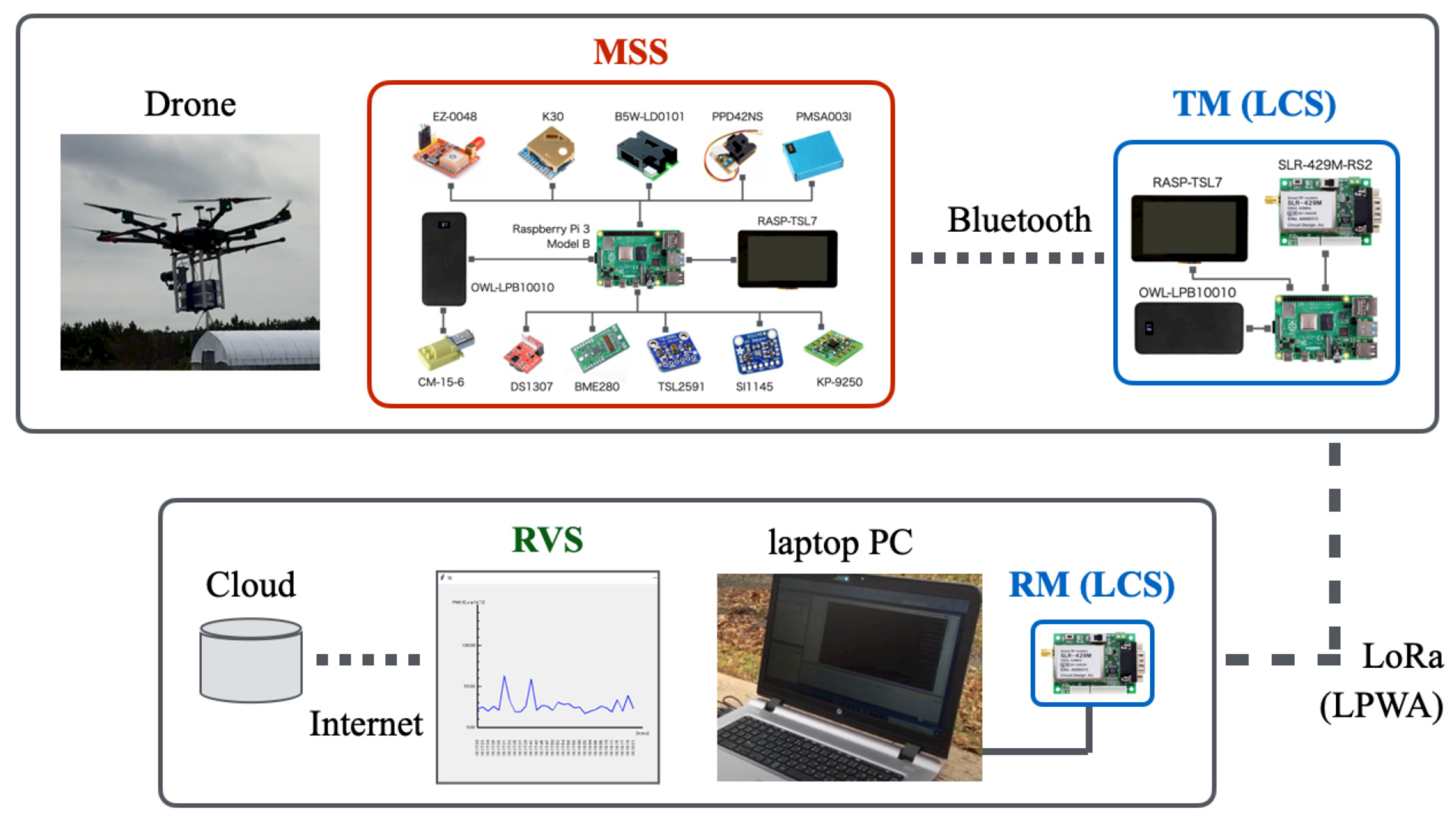
3.1. Overall System Architecture
3.2. Multiple Sensing of Atmosphere
3.2.1. Specifications
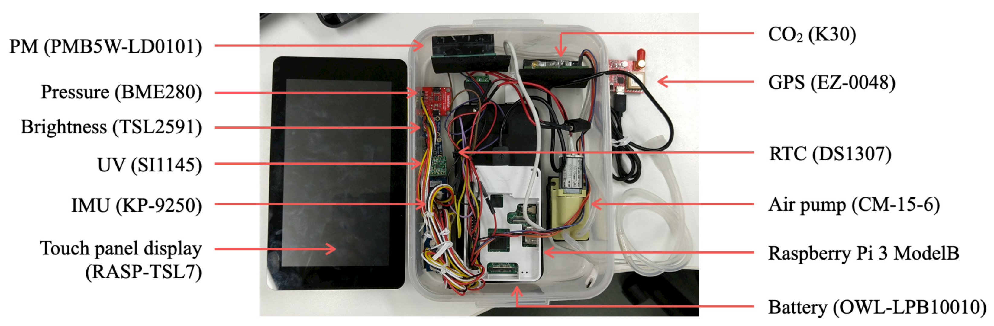
3.2.2. Assembly
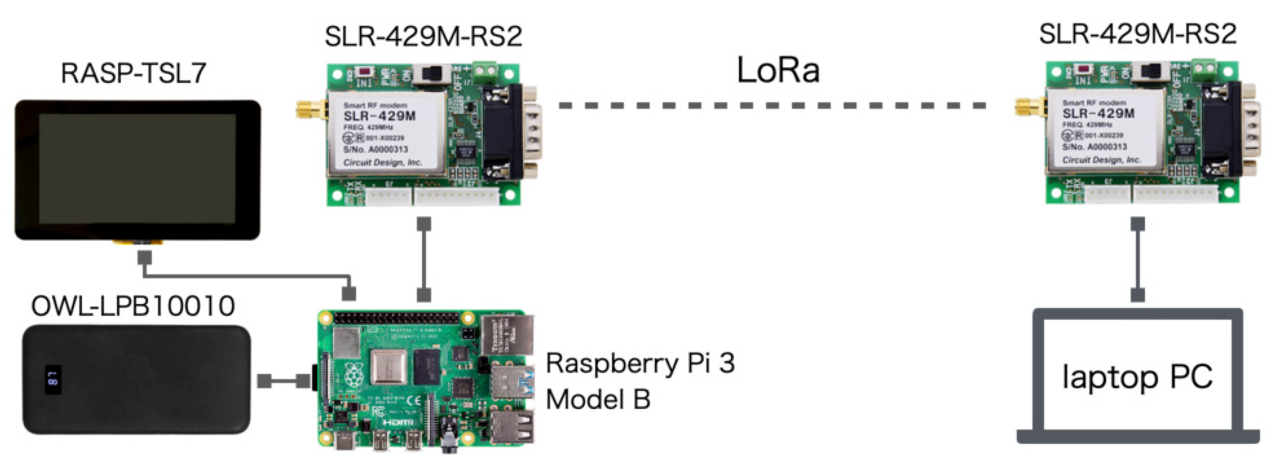
3.3. Long-Range Wireless Communication
3.4. Real-Time Monitoring and Visualization
3.5. Drone Mounting
3.5.1. Platform Drone
3.5.2. Originally Developed Sensor Brackets
4. Communication Experiment
4.1. Ground Communication Experiment
4.1.1. Setup
4.1.2. Results
4.2. Flight Communication Experiment
4.2.1. Setup
4.2.2. Results
5. Preliminary Sensor Comparison Experiment
5.1. Experiment Setup and Sensor Comparison
5.2. Calibration with AEROS
5.2.1. Setup
5.2.2. Results
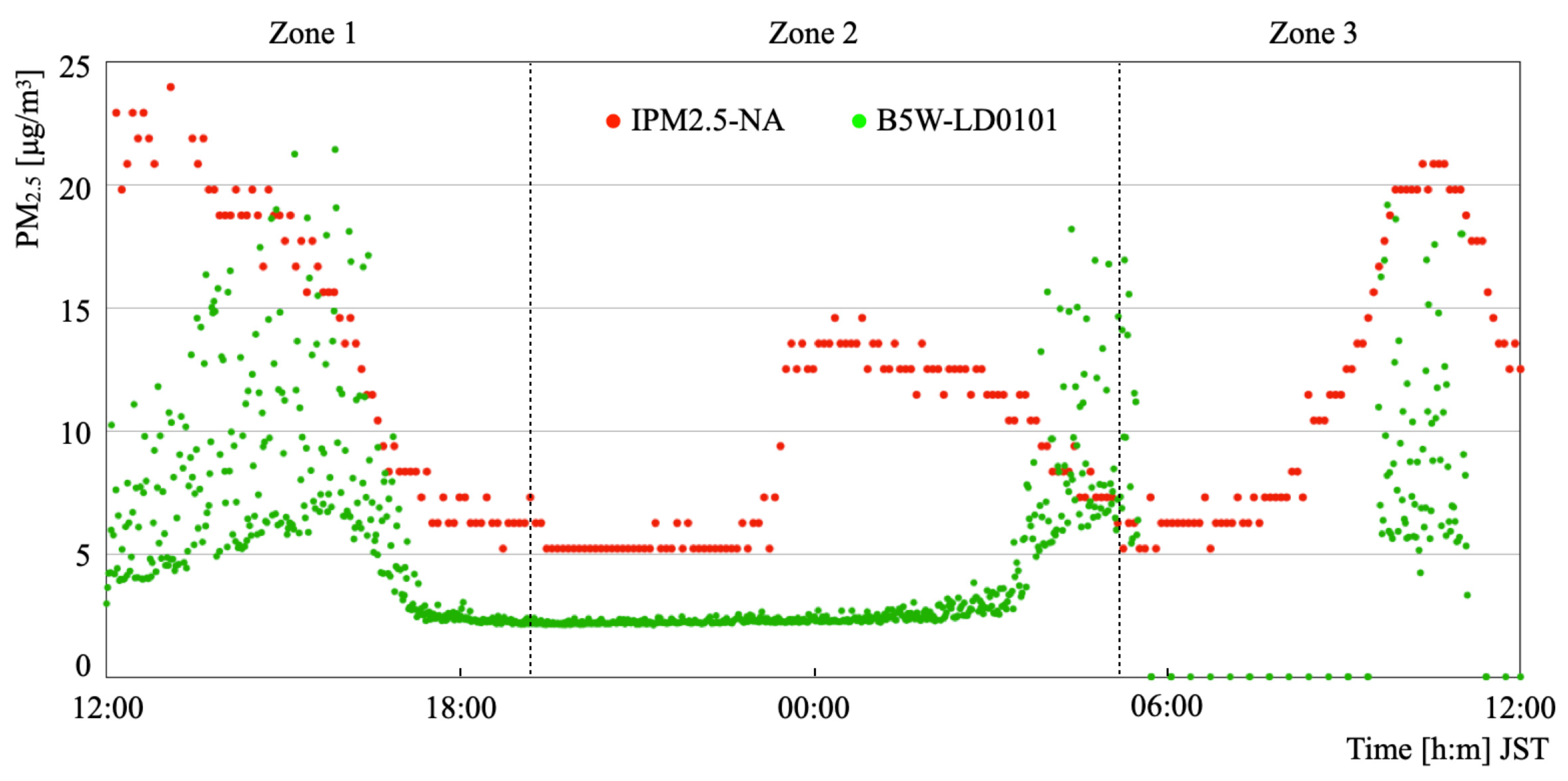
5.3. Calibration with IPM2.5-NA
5.3.1. Setup
5.3.2. Results
6. Application Experiments for Flight Measurement and Distribution Prediction
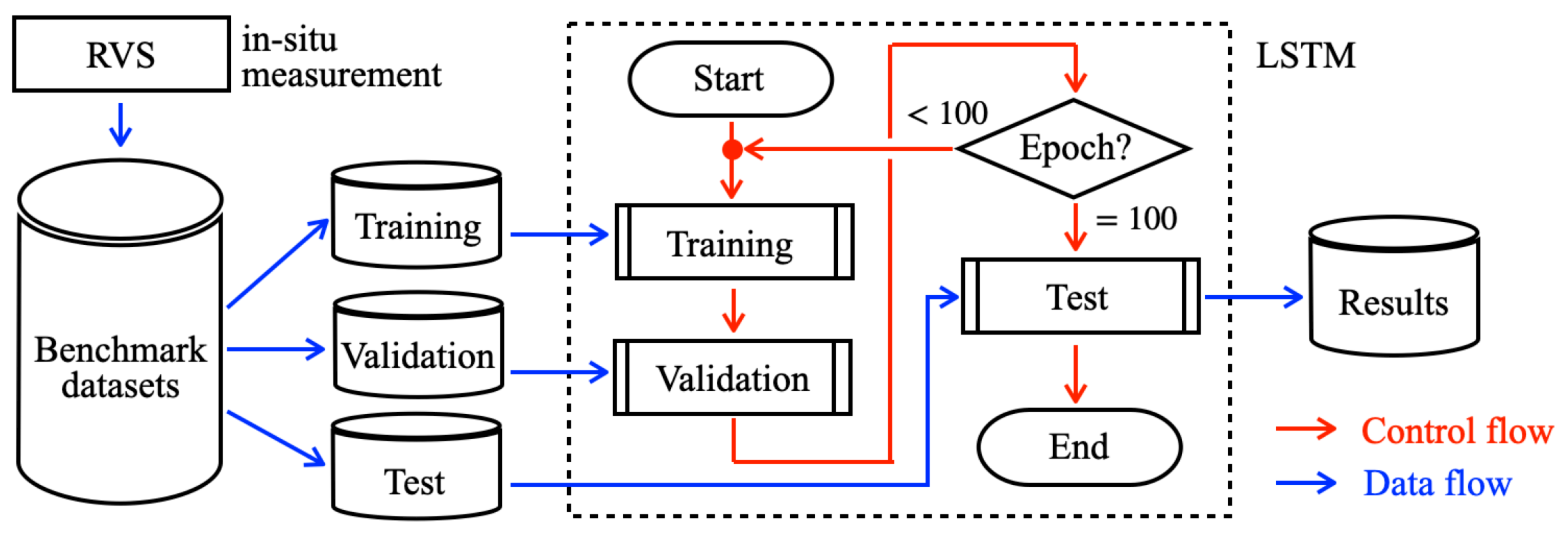
6.1. LSTM
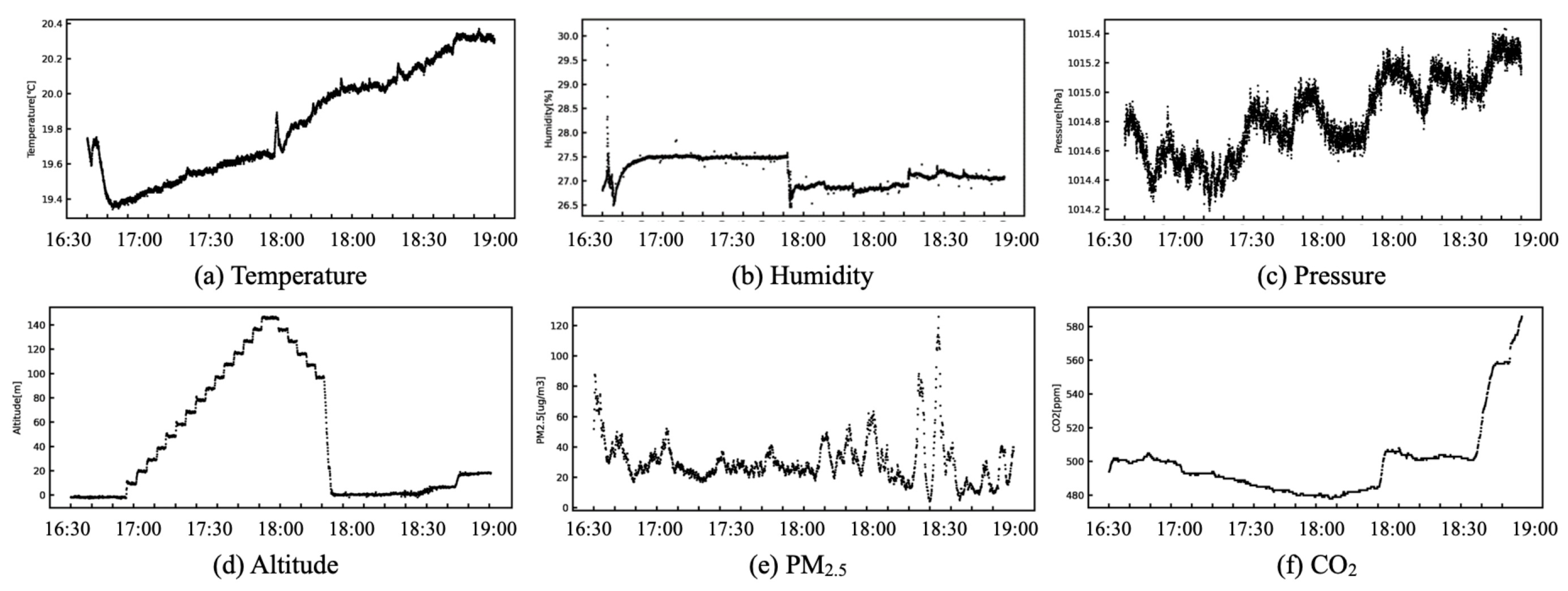
6.2. Measurement Flight Experiment Results
6.3. PM Concentration Prediction Results
7. Conclusions
Author Contributions
Funding
Institutional Review Board Statement
Informed Consent Statement
Data Availability Statement
Acknowledgments
Conflicts of Interest
Abbreviations
| ANN | Artificial neural network |
| AEROS | Atmospheric environmental regional observation system |
| CART | Classification and regression tree |
| CO | Carbon monoxide |
| CO | Carbon dioxide |
| CV | Cross-validation |
| DRNN | Deep recurrent neural networks |
| DTT | Dynamic pre-training |
| EELM | Ensemble extreme learning machine |
| FC | Fight controller |
| FPV | First person view |
| FRP | Fiber reinforced plastics |
| GBR | Gradient boosting regression |
| GBM | Gradient boosting machine |
| GPS | Global positioning system |
| GPIO | General-purpose input–output |
| GT | Ground truth |
| GUI | Graphical user interface |
| I2C | Inter-integrated circuit |
| IoT | Internet of things |
| IMU | Inertial measurement unit |
| INP | Ice nucleation particles |
| k-NN | k-nearest neighbor |
| LCS | Long-range wireless communication system |
| LiDAR | Light detection and ranging |
| LoRa | Long range |
| LPWA | Low power wide area |
| LPWAN | Low-power wide-area network |
| LSTM | Long short-term memory |
| MAE | Mean absolute error |
| MSS | Multi-sensor system |
| NBIoT | Narrow band-Internet of things |
| NDIR | Non-dispersive infrared |
| NO | Nitric oxide |
| NO | Nitrogen dioxide |
| OS | Operating system |
| PM | Particulate matter |
| PP | Polypropylene |
| PWM | Pulse width modulation |
| RF | Random forest |
| RM | Receiver module |
| RNN | Recurrent neural network |
| RTC | Real-time clock |
| RVS | Real-time visualization system |
| SBC | Single board computer |
| SfM | Structure from motion |
| SGD | Stochastic gradient descent |
| SVR | support vector regression |
| SVM | Support vector machine |
| TEOM | Tapered element oscillating microbalance |
| TM | Transmitter module |
| 3D | Three-dimensional |
| UAV | Unmanned aerial vehicles |
| UFP | Ultrafine particles |
| USB | Universal serial bus |
| UV | Ultraviolet |
References
- Meehl, G.A.; Washington, W.M.; Collins, W.D.; Arblaster, J.M.; Hu, A.; Buja, L.E.; Strand, W.G.; Teng, H. How Much More Global Warming and Sea Level Rise? Science 2005, 307, 1769–1772. [Google Scholar] [CrossRef] [Green Version]
- Landsea, C. Hurricanes and Global Warming. Nature 2005, 438, E11–E12. [Google Scholar] [CrossRef]
- Houghton, J. Global Warming. Rep. Prog. Phys. 2005, 68, 1343–1403. [Google Scholar] [CrossRef]
- Khandekar, M.L.; Murty, T.S.; Chittibabu, P. The Global Warming Debate: A Review of the State of Science. Pure Appl. Geophys. 2005, 162, 1557–1586. [Google Scholar] [CrossRef]
- Grennfelt, P.; Engleryd, A.; Forsius, M.; Hov, O.; Rodhe, H.; Cowling, E. Acid Rain and Air Pollution: 50 Years of Progress in Environmental Science and Policy. Ambio 2020, 49, 849–864. [Google Scholar] [CrossRef] [Green Version]
- Karagulian, F.; Belis, C.A.; Dora, C.F.C.; Prüss-Ustün, A.M.; Bonjour, S.; Adair-Rohani, H.; Amann, M. Contributions to Cities’ Ambient Particulate Matter (PM): A Systematic Review of Local Source Contributions at Global Level. Atmos. Environ. 2015, 120, 475–483. [Google Scholar] [CrossRef]
- Xing, Y.F.; Xu, Y.H.; Shi, M.H.; Lian, Y.X. The Impact of PM2.5 on the Human Respiratory System. J. Thorac. Dis. 2016, 8, E69–E74. [Google Scholar] [PubMed]
- Wang, C.; Tu, Y.; Yu, Z.; Lu, R. PM2.5 and Cardiovascular Diseases in the Elderly: An Overview. Int. J. Environ. Res. Public Health 2015, 12, 8187–8197. [Google Scholar] [CrossRef] [PubMed] [Green Version]
- Atkinson, R.W.; Kang, S.; Anderson, H.R.; Mills, I.C.; Walton, H.A. Epidemiological Time Series Studies of PM2.5 and Daily Mortality and Hospital Admissions: A Systematic Review and Meta-Analysis. Thorax 2014, 69, 660–665. [Google Scholar] [CrossRef] [PubMed] [Green Version]
- Nowak, D.J.; Hirabayashi, S.; Bodine, A.; Hoehn, R. Modeled PM2.5 Removal by Trees in Ten U.S. Cities and Associated Health Effects. Environ. Pollut. 2013, 178, 395–402. [Google Scholar] [CrossRef] [PubMed]
- Schlesinger, R.B. The Health Impact of Common Inorganic Components of Fine Particulate Matter (PM2.5) in Ambient Air: A Critical Review. Inhal. Toxicol. 2007, 19, 811–832. [Google Scholar] [CrossRef]
- Gelencsér, A.; May, B.; Simpson, D.; Sánchez-Ochoa, A.; Kasper-Giebl, A.; Puxbaum, H.; Caseiro, A.; Pio, C.; Legrand, M. Source Apportionment of PM2.5 Organic Aerosol Over Europe: Primary/Secondary, Natural/Anthropogenic, and Fossil/Biogenic Origin. J. Geophys. Res. 2007, 112, D23S04. [Google Scholar] [CrossRef] [Green Version]
- Iriti, M.; Piscitelli, P.; Missoni, E.; Miani, A. Air Pollution and Health: The Need for a Medical Reading of Environmental Monitoring Data. Int. J. Environ. Res. Public Health 2020, 17, 2174. [Google Scholar] [CrossRef] [Green Version]
- Liu, D.; Zhang, Q.; Jiang, J.; Chen, D.R. Performance Calibration of Low-Cost and Portable Particular Matter (PM) Sensors. J. Aerosol Sci. 2017, 112, 1–10. [Google Scholar] [CrossRef]
- Nakayama, T.; Matsumi, Y.; Kawahito, K.; Watabe, Y. Development and Evaluation of a Palm-Sized Optical PM2.5 Sensor. Aerosol Sci. Technol. 2018, 52, 1. [Google Scholar] [CrossRef] [Green Version]
- Kuula, J.; Mäkelä, T.; Aurela, M.; Teinilä, K.; Varjonen, S.; González, O.; Timonen, H. Laboratory Evaluation of Particle-Size Selectivity of Optical Low-Cost Particulate Matter Sensors. Atmos. Meas. Tech. 2020, 13, 2413–2423. [Google Scholar] [CrossRef]
- Sasaki, K.; Inoue, M.; Shimura, T.; Iguchi, M. In Situ, Rotor-Based Drone Measurement of Wind Vector and Aerosol Concentration in Volcanic Areas. Atmosphere 2021, 12, 376. [Google Scholar] [CrossRef]
- Inoue, M.; Haga, Y.; Nagayoshi, T.; Madokoro, H.; Takakai, F.; Kiguchi, O.; Morino, I. Measurement of Atmospheric Carbon Dioxide Using Unmanned Aerial Vehicle for Profiling Vertical Distribution over Akita. In Proceedings of the 14th International Commission on Atmospheric Chemistry and Global Pollution, Kagawa, Japan, 25–29 September 2018. [Google Scholar]
- Haga, Y.; Chiba, T.; Inoue, M.; Kiguchi, O.; Nagayoshi, T.; Madokoro, H.; Ise, T.; Abe, M.; Morino, I.; Sasakawa, M.; et al. Regional Atmospheric CO2 Concentration Detected by NDIR Onboard a UAV in the Lower Part of Neutrally Atmospheric Boundary Layers in Ogata, Akita, Japan. In Proceedings of the International Symposium on Agricultural Meteorology, Shizuoka, Japan, 27–29 March 2019. [Google Scholar]
- Chiba, T.; Haga, Y.; Inoue, M.; Kiguchi, O.; Nagayoshi, T.; Madokoro, H. Morino, I. Detecting Regional Atmospheric CO2 Concentrations in the Lower Troposphere with an NDIR Mounted on a UAV, Ogata Village, Akita, Japan. Atmosphere 2019, 10, 487. [Google Scholar] [CrossRef] [Green Version]
- Nomura, K.; Madokoro, H.; Chiba, T.; Inoue, M.; Nagayoshi, T.; Kiguchi, O.; Woo, H.; Sato, K. Operation and Maintenance of In-Situ CO2 Measurement System Using Unmanned Aerial Vehicles. In Proceedings of the 19th International Conference on Control, Automation and Systems, Jeju, Korea, 15–18 October 2019; pp. 992–997. [Google Scholar]
- Madokoro, H.; Inoue, M.; Nagayoshi, T.; Chiba, T.; Haga, Y.; Kiguchi, O.; Sato, K. Prototype Development of Drone System Used for In-situ Measurement of CO2 Vertical Profile and Its Preliminary Flight Test. Trans. Soc. Instrum. Control Eng. 2020, 56, 37–44. [Google Scholar] [CrossRef]
- Shibata, Y.; Nagasawa, C.; Abo, M.; Inoue, M.; Morino, I.; Uchino, O. Comparison of CO2 Vertical Profiles in the Lower Troposphere between 1.6 μm Differential Absorption Lidar and Aircraft Measurements Over Tsukuba. Sensors 2018, 18, 4064. [Google Scholar] [CrossRef] [Green Version]
- Inai, Y.; Aoki, S.; Honda, H.; Furutani, H.; Matsumi, Y.; Ouchi, M.; Sugawara, S.; Hasebe, F.; Uematsu, M.; Fujiwara, M. Balloon-Borne Tropospheric CO2 Observations Over the Equatorial Eastern and Western Pacific. Atmos. Environ. 2018, 184, 24–36. [Google Scholar] [CrossRef]
- Toro, F.G.; Tsourdos, A. UAV or Drones for Remote Sensing Applications; MDPI Books: Basel, Switzerland, 2021; pp. 1–2. [Google Scholar]
- Yao, H.; Qin, R.; Chen, X. Unmanned Aerial Vehicle for Remote Sensing Applications—Review. Remote Sens. 2019, 11, 1443. [Google Scholar] [CrossRef] [Green Version]
- Pajares, G. Overview and Current Status of Remote Sensing Applications Based on Unmanned Aerial Vehicles (UAVs). Photogramm. Eng. Remote Sens. 2015, 81, 281–330. [Google Scholar] [CrossRef] [Green Version]
- Madokoro, H.; Sato, K.; Shimoi, N. Vision-Based Indoor Scene Recognition from Time-Series Aerial Images Obtained Using a MAV Mounted Monocular Camera. Drones 2019, 3, 22. [Google Scholar] [CrossRef] [Green Version]
- Mlambo, R.; Woodhouse, I.H.; Gerard, F.; Anderson, K. Structure from Motion (SfM) Photogrammetry with Drone Data: A Low Cost Method for Monitoring Greenhouse Gas Emissions from Forests in Developing Countries. Forests 2017, 8, 68. [Google Scholar] [CrossRef] [Green Version]
- Kelly, J.; Kljun, N.; Olsson, P.-O.; Mihai, L.; Liljeblad, B.; Weslien, P.; Klemedtsson, L.; Eklundh, L. Challenges and Best Practices for Deriving Temperature Data from an Uncalibrated UAV Thermal Infrared Camera. Remote Sens. 2019, 11, 567. [Google Scholar] [CrossRef] [Green Version]
- Wu, X.; Shen, X.; Cao, L.; Wang, G.; Cao, F. Assessment of Individual Tree Detection and Canopy Cover Estimation using Unmanned Aerial Vehicle based Light Detection and Ranging (UAV-LiDAR) Data in Planted Forests. Remote Sens. 2019, 11, 908. [Google Scholar] [CrossRef] [Green Version]
- Pellicani, R.; Argentiero, I.; Manzari, P.; Spilotro, G.; Marzo, C.; Ermini, R.; Apollonio, C. UAV and Airborne LiDAR Data for Interpreting Kinematic Evolution of Landslide Movements: The Case Study of the Montescaglioso Landslide (Southern Italy). Geosciences 2019, 9, 248. [Google Scholar] [CrossRef] [Green Version]
- Christiansen, M.P.; Laursen, M.S.; Jørgensen, R.N.; Skovsen, S.; Gislum, R. Designing and Testing a UAV Mapping System for Agricultural Field Surveying. Sensors 2017, 17, 2703. [Google Scholar] [CrossRef] [Green Version]
- Brede, B.; Lau, A.; Bartholomeus, H.M.; Kooistra, L. Comparing RIEGL RiCOPTER UAV LiDAR Derived Canopy Height and DBH with Terrestrial LiDAR. Sensors 2017, 17, 2371. [Google Scholar] [CrossRef]
- de Boer, G.; Houston, A.; Jacob, J.; Chilson, P.B.; Smith, S.W.; Argrow, B.; Lawrence, D.; Elston, J.; Brus, D.; Kemppinen, O.; et al. Data generated during the 2018 LAPSE-RATE campaign: An introduction and overview. Earth Syst. Sci. Data 2020, 12, 3357–3366. [Google Scholar] [CrossRef]
- de Boer, G.; Dixon, C.; Borenstein, S.; Lawrence, D.A.; Elston, J.; Hesselius, D.; Stachura, M.; Laurence, R., III; Swenson, S.; Choate, C.M.; et al. University of Colorado and Black Swift Technologies RPAS-based measurements of the lower atmosphere during LAPSE-RATE. Earth Syst. Sci. Data 2021, 13, 2515–2528. [Google Scholar] [CrossRef]
- Hassanalian, M.; Abdelkefi, A. Classifications, Applications, and Design Challenges of Drones: A Review. Prog. Aerosp. Sci. 2017, 91, 99–131. [Google Scholar] [CrossRef]
- Villa, T.F.; Gonzalez, F.; Miljievic, B.; Ristovski, Z.D.; Morawska, L. An Overview of Small Unmanned Aerial Vehicles for Air Quality Measurements: Present Applications and Future Prospectives. Sensors 2016, 16, 1072. [Google Scholar] [CrossRef] [PubMed] [Green Version]
- Juan, R.; Joossen, G.; Sanz, D.; del Cerro, J.; Barrientos, A. Mini-UAV Based Sensory System for Measuring Environmental Variables in Greenhouses. Sensors 2015, 15, 3334–3350. [Google Scholar]
- Rossi, M.; Brunelli, D. Autonomous Gas Detection and Mapping With Unmanned Aerial Vehicles. IEEE Trans. Instrum. Meas. 2016, 65, 765–775. [Google Scholar] [CrossRef]
- Villa, T.F.; Salimi, F.; Morton, K.; Morawska, L.; Gonzalez, F. Development and Validation of a UAV Based System for Air Pollution Measurements. Sensors 2016, 16, 2202. [Google Scholar] [CrossRef] [Green Version]
- Ishihara, H.; Tateyama, K.; Satoh, T.; Kobayashi, K. A Case Study on the Occurrence Situation of the Superior Mirage Using UAV. In Proceedings of the JSSI & JSSE Joint Conference on Snow and Ice Research, Toyama, Japan, 24–27 September 2017; pp. 21–24. [Google Scholar]
- Inoue, M.; Sasaki, K.; Kobayashi, T.; Tsujimoto, H.; Shimura, T. Feasibility Study of Upper Air Observation Method Using Drone. In Proceedings of the Annual Conference, Japan Society of Hydrology and Water Resources, Hokkaido, Japan, 19–21 September 2017; pp. 52–53. [Google Scholar]
- Chang, C.C.; Chang, C.Y.; Wang, J.L.; Lin, M.R.; Ou-Yang, C.F.; Pan, H.H.; Chen, Y.C. A Study of Atmospheric Mixing of Trace Gases by Aerial Sampling with a Multi-Rotor Drone. Atmos. Environ. 2018, 184, 254–261. [Google Scholar] [CrossRef]
- Andersen, T.; Scheeren, B.; Peters, W.; Chen, H. A UAV-Based Active AirCore System for Measurements of Greenhouse Gases. Atmos. Meas. Tech. 2018, 11, 2683–2699. [Google Scholar] [CrossRef] [Green Version]
- Karion, A.; Sweeney, C.; Tans, P.; Newberger, T. AirCore: An Innovative Atmospheric Sampling System. J. Atmos. Ocean. Technol. 2010, 27, 1839–1853. [Google Scholar] [CrossRef]
- Rüdiger, J.; Tirpitz, J.L.; Moor, J.M.; Bobrowski, N.; Gutmann, A.; Liuzzo, M.; Ibarra, M.; Hoffmann, T. Implementation of Electrochemical, Optical and Denuder-Based Sensors and Sampling Techniques on UAV for Volcanic Gas Measurements: Examples from Masaya, Turrialba and Stromboli volcanoes. Atmos. Meas. Tech. 2018, 11, 2441–2457. [Google Scholar] [CrossRef] [Green Version]
- Weber, K.; Heweling, G.; Fischer, C.; Lange, M. The Use of an Octocopter UAV for the Determination of Air Pollutants—Case Study of the Traffic Induced Pollution Plume Around a River Bridge in Duesseldorf, Germany. Int. J. Environ. Sci. 2017, 2, 63–66. [Google Scholar]
- Meier, L.; Tanskanen, P.; Fraundorfer, F.; Pollefeys, M. PIXHAWK: A System for Autonomous Flight Using Onboard Computer Vision. In Proceedings of the IEEE International Conference on Robotics and Automation, Shanghai, China, 9–13 May 2011; pp. 2992–2997. [Google Scholar]
- Peters, T.M.; Ott, D.; O’shaughnessy, P.T. Comparison of the Grimm 1.108 and 1.109 Portable Aerosol Spectrometer to the TSI 3321 Aerodynamic Particle Sizer for Dry Particles. Ann. Occup. Hyg. 2006, 50, 843–850. [Google Scholar]
- Wang, T.; Han, W.; Zhang, M.; Yao, X.; Zhang, L.; Peng, X.; Li, C.; Dan, X. Unmanned Aerial Vehicle-Borne Sensor System for Atmosphere–Particulate–Matter Measurements: Design and Experiments. Sensors 2020, 20, 57. [Google Scholar] [CrossRef] [Green Version]
- Okamura, K.; Takagi, S.; Ito, M.; Lin, J.S. A Study on Spatial Representativeness of CO2 Concentration—Toward to Environmental Education Program Using a Drone. Bull. Inst. Environ. Manag. 2020, 19, 4–9. [Google Scholar]
- Bieber, P.; Seifried, T.M.; Burkart, J.; Gratzl, J.; Kasper-Giebl, A.; Schmale, D.G., III; Grothe, H. A Drone-Based Bioaerosol Sampling System to Monitor Ice Nucleation Particles in the Lower Atmosphere. Remote Sens. 2020, 12, 552. [Google Scholar] [CrossRef] [Green Version]
- Islam, N.; Rashid, M.M.; Pasandideh, F.; Ray, B.; Moore, S.; Kadel, R. A Review of Applications and Communication Technologies for Internet of Things (IoT) and Unmanned Aerial Vehicle (UAV) Based Sustainable Smart Farming. Sustainability 2021, 13, 1821. [Google Scholar] [CrossRef]
- Furquim, G.; Filho, G.P.R.; Jalali, R.; Pessin, G.; Pazzi, R.W.; Ueyama, J. How to Improve Fault Tolerance in Disaster Predictions: A Case Study about Flash Floods Using IoT, ML and Real Data. Sensors 2018, 18, 907. [Google Scholar] [CrossRef] [PubMed] [Green Version]
- Tong, X.; Yang, H.; Wang, L.; Miao, Y. The Development and Field Evaluation of an IoT System of Low-Power Vibration for Bridge Health Monitoring. Sensors 2019, 19, 1222. [Google Scholar] [CrossRef] [PubMed] [Green Version]
- Ragnoli, M.; Barile, G.; Leoni, A.; Ferri, G.; Stornelli, V. An Autonomous Low-Power LoRa-Based Flood-Monitoring System. J. Low Power Electron. Appl. 2020, 10, 15. [Google Scholar] [CrossRef]
- Haque, M.E.; Asikuzzaman, M.; Khan, I.U.; Ra, I.-H.; Hossain, M.S.; Shah, S.B.H. Comparative Study of IoT-Based Topology Maintenance Protocol in a Wireless Sensor Network for Structural Health Monitoring. Remote Sens. 2020, 12, 2358. [Google Scholar] [CrossRef]
- Kim, K.; Li, S.; Heydariaan, M.; Smaoui, N.; Gnawali, O.; Suh, W.; Suh, M.J.; Kim, J.I. Feasibility of LoRa for Smart Home Indoor Localization. Appl. Sci. 2021, 11, 415. [Google Scholar] [CrossRef]
- Lagkas, T.; Argyriou, V.; Bibi, S.; Sarigiannidis, P. UAV IoT Framework Views and Challenges: Towards Protecting Drones as ‘Things’. Sensors 2018, 18, 4015. [Google Scholar] [CrossRef] [PubMed] [Green Version]
- Dambal, V.A.; Mohadikar, S.; Kumbhar, A.; Guvenc, I. Improving LoRa Signal Coverage in Urban and Sub-Urban Environments with UAVs. In Proceedings of the International Workshop on Antenna Technology, Miami, FL, USA, 3–6 March 2019; pp. 210–213. [Google Scholar]
- Saraereh, O.A.; Alsaraira, A.; Khan, I.; Uthansakul, P. Performance Evaluation of UAV-Enabled LoRa Networks for Disaster Management Applications. Sensors 2020, 20, 2396. [Google Scholar] [CrossRef]
- Chen, L.; Huang, H.; Wu, C.; Tsai, Y.; Chang, Y. A LoRa-Based Air Quality Monitor on Unmanned Aerial Vehicle for Smart City. In Proceedings of the International Conference on System Science and Engineering, New Taipei, Taiwan, 28–30 June 2018; pp. 1–5. [Google Scholar]
- Masood, A.; Ahmad, K. A Model for Particulate Matter (PM2.5) Prediction for Delhi Based on Machine Learning Approaches. Procedia Comput. Sci. 2020, 167, 2101–2110. [Google Scholar] [CrossRef]
- Doreswamy, N.; Harishkumar, K.S.; Yogesh, K.M.; Ibrahim, G. Forecasting Air Pollution Particulate Matter (PM2.5) Using Machine Learning Regression Models. Procedia Comput. Sci. 2020, 171, 2057–2066. [Google Scholar] [CrossRef]
- Danesh Yazdi, M.; Kuang, Z.; Dimakopoulou, K.; Barratt, B.; Suel, E.; Amini, H.; Lyapustin, A.; Katsouyanni, K.; Schwartz, J. Predicting Fine Particulate Matter (PM2.5) in the Greater London Area: An Ensemble Approach using Machine Learning Methods. Remote Sens. 2020, 12, 914. [Google Scholar] [CrossRef] [Green Version]
- Sugiura, K.; Theang, O.B.; Zettsu, K. Predicting Environment Monitoring Data by Deep Recurrent Neural Networks. In Proceedings of the 29th Annual Conference of the Japanese Society for Artificial Intelligence, Hakodate, Japan, 30 February–2 June 2015. [Google Scholar]
- Song, S.; Lam, J.C.K.; Han, Y.; Li, V.O.K. ResNet-LSTM for Real-Time PM2.5 and PM10 Estimation Using Sequential Smartphone Images. IEEE Access 2020, 8, 220069–220082. [Google Scholar] [CrossRef]
- He, K.; Zhang, X.; Ren, S.; Sun, J. Deep Residual Learning for Image Recognition. In Proceedings of the IEEE Conference on Computer Vision and Pattern Recognition, Las Vegas, NV, USA, 26–30 June 2016; pp. 770–778. [Google Scholar]
- Shang, Z.; Deng, T.; He, J.; Duan, X. A Novel Model for Hourly PM2.5 Concentration Prediction Based on CART and EELM. Sci. Total Environ. 2019, 651, 3043–3052. [Google Scholar] [CrossRef]
- Breiman, L.; Friedman, J.H.; Olshen, R.; Stone, C.J. Classification and Regression Trees. Biometrics 1984, 40, 358. [Google Scholar]
- Xue, X.W.; Yao, M.; Wu, Z.H.; Yang, J.H. Genetic Ensemble of Extreme Learning Machine. Neurocomputing 2014, 129, 175–184. [Google Scholar] [CrossRef]
- Bisdikian, C. An Overview of the Bluetooth Wireless Technology. IEEE Commun. Mag. 2001, 39, 86–94. [Google Scholar] [CrossRef] [Green Version]
- Venkatraman Jagatha, J.; Klausnitzer, A.; Chacón-Mateos, M.; Laquai, B.; Nieuwkoop, E.; van der Mark, P.; Vogt, U.; Schneider, C. Calibration Method for Particulate Matter Low-Cost Sensors Used in Ambient Air Quality Monitoring and Research. Sensors 2021, 21, 3960. [Google Scholar] [CrossRef]
- Dinh, T.-V.; Choi, I.-Y.; Son, Y.-S.; Kim, J.-C. A Review on Non-Dispersive Infrared Gas Sensors: Improvement of Sensor Detection Limit and Interference Correction. Sens. Actuators B Chem. 2016, 231, 529–538. [Google Scholar] [CrossRef]
- Holtz, J. Pulsewidth Modulation—A Survey. IEEE Trans. Ind. Electron. 1992, 39, 410–420. [Google Scholar] [CrossRef]
- Yang, F.; Xue, X.; Cai, C.; Sun, Z.; Zhou, Q. Numerical Simulation and Analysis on Spray Drift Movement of Multirotor Plant Protection Unmanned Aerial Vehicle. Energies 2018, 11, 2399. [Google Scholar] [CrossRef] [Green Version]
- Wu, Y.; Qi, L.; Zhang, H.; Musiu, E.M.; Yang, Z.; Wang, P. Design of UAV Downwash Airflow Field Detection System Based on Strain Effect Principle. Sensors 2019, 19, 2630. [Google Scholar] [CrossRef] [PubMed] [Green Version]
- Sinha, R.S.; Wei, Y.; Hwang, S.-H. A Survey on LPWA Technology: LoRa and NB-IoT. ICT Express 2017, 3, 14–21. [Google Scholar] [CrossRef]
- Popli, S.; Jha, R.K.; Jain, S. A Survey on Energy Efficient Narrowband Internet of Things (NBIoT): Architecture, Application and Challenges. IEEE Access 2019, 7, 16739–16776. [Google Scholar] [CrossRef]
- Poursafar, N.; Alahi, M.E.E.; Mukhopadhyay, S. Long-Range Wireless Technologies for IoT Applications: A Review. In Proceedings of the Eleventh International Conference on Sensing Technology, Sydney, NSW, Australia, 4–6 December 2017; pp. 1–6. [Google Scholar]
- Pereira, L.G.; Fernandez, P.; Mourato, S.; Matos, J.; Mayer, C.; Marques, F. Quality Control of Outsourced LiDAR Data Acquired with a UAV: A Case Study. Remote Sens. 2021, 13, 419. [Google Scholar] [CrossRef]
- Cichowicz, R.; Dobrzański, M. Spatial Analysis (Measurements at Heights of 10 m and 20 m above Ground Level) of the Concentrations of Particulate Matter (PM10, PM2.5, and PM1.0) and Gaseous Pollutants (H2S) on the University Campus: A Case Study. Atmosphere 2021, 12, 62. [Google Scholar] [CrossRef]
- Morales, A.; Guerra, R.; Horstrand, P.; Diaz, M.; Jimenez, A.; Melian, J.; Lopez, S.; Lopez, J.F. A Multispectral Camera Development: From the Prototype Assembly until Its Use in a UAV System. Sensors 2020, 20, 6129. [Google Scholar] [CrossRef]
- Martinez, B.; Miller, T.W.; Yalin, A.P. Cavity Ring-Down Methane Sensor for Small Unmanned Aerial Systems. Sensors 2020, 20, 454. [Google Scholar] [CrossRef] [Green Version]
- Rogers, S.R.; Manning, I.; Livingstone, W. Comparing the Spatial Accuracy of Digital Surface Models from Four Unoccupied Aerial Systems: Photogrammetry Versus LiDAR. Remote Sens. 2020, 12, 2806. [Google Scholar] [CrossRef]
- Deng, X.; Zhu, Z.; Yang, J.; Zheng, Z.; Huang, Z.; Yin, X.; Wei, S.; Lan, Y. Detection of Citrus Huanglongbing Based on Multi-Input Neural Network Model of UAV Hyperspectral Remote Sensing. Remote Sens. 2020, 12, 2678. [Google Scholar] [CrossRef]
- Canisius, F.; Wang, S.; Croft, H.; Leblanc, S.G.; Russell, H.A.J.; Chen, J.; Wang, R. A UAV-Based Sensor System for Measuring Land Surface Albedo: Tested over a Boreal Peatland Ecosystem. Drones 2019, 3, 27. [Google Scholar] [CrossRef] [Green Version]
- Bielsa, G.; Mezzavilla, M.; Widmer, J.; Rangan, S. Performance Assessment of Off-The-Shelf MM Wave Radios for Drone Communications. In Proceedings of the IEEE 20th International Symposium on A World of Wireless, Mobile and Multimedia Networks, Washington, DC, USA, 10–12 June 2019; pp. 1–3. [Google Scholar]
- Zhou, G.; Bao, X.; Ye, S.; Wang, H.; Yan, H. Selection of Optimal Building Facade Texture Images From UAV-Based Multiple Oblique Image Flows. IEEE Trans. Geosci. Remote Sens. 2021, 59, 1534–1552. [Google Scholar] [CrossRef]
- Ferreira, M.E.; Alves, L.R.; Albuquerque, R.W.; Broadbent, E.; Almeida, D.R.A.; Avino, F.S.; Cezare, C.H.G.; Zambrano, A.M.A.; Wilkinson, B.; Oliveira-da-Costa, M. Monitoring The Brazilian Savanna with LIDAR and RGB Sensors Onboard Remotely Piloted Aircraft Systems. In Proceedings of the IEEE International Geoscience and Remote Sensing Symposium, Yokohama, Japan, 28 July–2 August 2019; pp. 9240–9243. [Google Scholar]
- Horstrand, P.; Guerra, R.; Rodríguez, A.; Díaz, M.; López, S.; López, J.F. A UAV Platform Based on a Hyperspectral Sensor for Image Capturing and On-Board Processing. IEEE Access 2019, 7, 66919–66938. [Google Scholar] [CrossRef]
- Patashnick, H.; Meyer, M.; Rogers, B. Tapered Element Oscillating Microbalance Technology. In Proceedings of the North American/Ninth US Mine Ventilation Symposium, Kingston, ON, Canada, 8–12 June 2002; pp. 625–631. [Google Scholar]
- Hochreiter, S.; Schmidhuber, J. Long Short-Term Memory. Neural Comput. 1997, 9, 1735–1780. [Google Scholar] [CrossRef]
- Hochreiter, S. The Vanishing Gradient Problem During Learning Recurrent Neural Nets and Problem Solutions. Int. J. Uncertainty Fuzziness Knowl.-Based Syst. 1998, 6, 107–116. [Google Scholar] [CrossRef] [Green Version]
- Liu, L.; Liu, W.; Zheng, Y.; Ma, H.; Zhang, C. Third-Eye: A Mobilephone-Enabled Crowdsensing System for Air Quality Monitoring. In Proceedings of the ACM on Interactive, Mobile, Wearable and Ubiquitous Technologies, Singapore, 8–12 October 2018; pp. 1–26. [Google Scholar]
- Chen, R.; Wang, X.; Zhang, W.; Zhu, X.; Li, A.; Yang, C. A Hybrid CNN-LSTM Model for Typhoon Formation Forecasting. GeoInformatica 2019, 23, 375–396. [Google Scholar] [CrossRef]
- Huang, C.-J.; Kuo, P.-H. A Deep CNN-LSTM Model for Particulate Matter (PM2.5) Forecasting in Smart Cities. Sensors 2018, 18, 2220. [Google Scholar] [CrossRef] [PubMed] [Green Version]
- Zhang, T.; Song, S.; Li, S.; Ma, L.; Pan, S.; Han, L. Research on Gas Concentration Prediction Models Based on LSTM Multidimensional Time Series. Energies 2019, 12, 161. [Google Scholar] [CrossRef] [Green Version]
- Karim, F.; Majumdar, S.; Darabi, H.; Chen, S. LSTM Fully Convolutional Networks for Time Series Classification. IEEE Access 2018, 6, 1662–1669. [Google Scholar] [CrossRef]
- Bottou, L. Stochastic Gradient Descent Tricks. In Neural Networks: Tricks of the Trade; Springer: Berlin/Heidelberg, Germany, 2012; Volume 7700, pp. 421–436. [Google Scholar]
- Tieleman, T.; Hinton, G. Lecture 6.5–RMSProp: Divide the Gradient by a Running Average of its Recent Magnitude. COURSERA Neural Netw. Mach. Learn. 2012, 4, 26–31. [Google Scholar]
- Xu, D.; Zhang, S.; Zhang, H.; Mandic, D.P. Convergence of RMSProp Deep Learning Method with Penalty for Nonconvex Optimization. Neural Netw. 2021, 139, 17–23. [Google Scholar] [CrossRef]
- Zou, F.; Shen, L.; Jie, Z.; Zhang, W.; Liu, W. A Sufficient Condition for Convergences of Adam and RMSProp. In Proceedings of the IEEE/CVF Conference on Computer Vision and Pattern Recognition, Long Beach, CA, USA, 16–20 June 2019; pp. 11127–11135. [Google Scholar]
- Cortez, B.; Carrera, B.; Kim, Y.-J.; Jung, J.-Y. An Architecture for Emergency Event Prediction Using LSTM Recurrent Neural Networks. Expert Syst. Appl. 2018, 97, 315–324. [Google Scholar] [CrossRef]


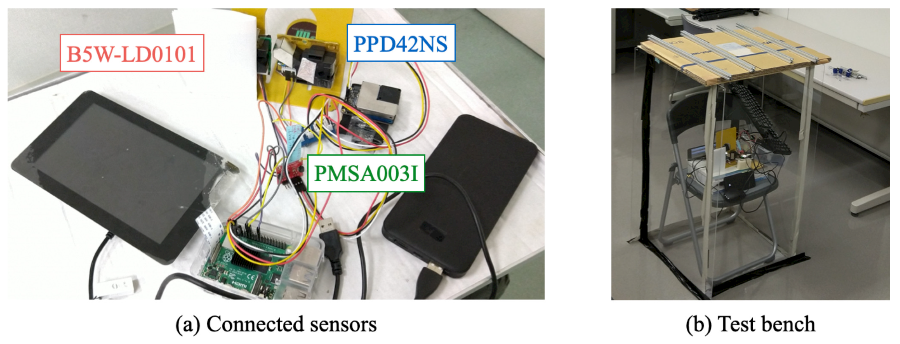
| Target | Model Name | Manufacturer |
|---|---|---|
| PM | B5W-LD0101 | Omron Corporation, Kyoto, Japan |
| PM | PPD42NS | Shinyei Technology Co., Ltd., Kobe, Japan |
| PM | PMSA003I | Beijing Plantower Co., Ltd., Beijing, China |
| CO | K30 | Senseair AB, Delsbo Sweden |
| GPS | L80-R (SKU:EZ-0048) | Quectel Wireless Solutions Co., Ltd., Shanghai, China |
| Humidity and pressure | BME280 | Robert Bosch GmbH, Stuttgart, Germany |
| Ambient light | TSL2591 | ams AG, Premstätten, Austria |
| UV | SI1145 | Adafruit Industries, New York, NY, USA |
| IMU | KP-9250 | Kyohritsu Electronic Industry Co., Ltd., Osaka, Japan |
| RTC | DS1307 | Adafruit Industries, New York, NY, USA |
| Air pump | CM-15-6 | Enomoto Micro Pump Mfg. Co., Ltd., Tokyo, Japan |
| SBC | Raspberry Pi 3 Model B | Raspberry Pi Foundation, Cambridge, UK |
| Touch panel display | RASP-TSL7 | Raspberry Pi Foundation, Cambridge, UK |
| Battery | OWL-LPB10010 | Owltech Co., Ltd., Kyoto City, Japan |
| Parameter | B5W-LD0101 | PPD42NS | PMSA003I |
|---|---|---|---|
| Manufacture | Omron | Shinyei Technology | Beijing Plantower |
| Sensor Type | Light scattering photometer | ||
| Detectable size range | 0.5 m | 1.0 m | 0.3 m |
| Size (H × W × D) | 52 × 39 × 18 mm | 59 × 42 × 22 mm | 51 × 36 × 14 mm |
| Weight | 20 g | 20 g | 28 g |
| Type | Wide [mm] | Long [mm] | High [mm] | Weight [kg] | Camera |
|---|---|---|---|---|---|
| 1 | 160 | 235 | 195 | 0.45 | unmount |
| 2 | 160 | 235 | 190 | 0.94 | unmount |
| 3 | 160 | 235 | 350 | 1.24 | mount |
| 4 | 180 | 290 | 270 | 1.83 | mount |
| 5 | 160 | 235 | 350 | 0.99 | mount |
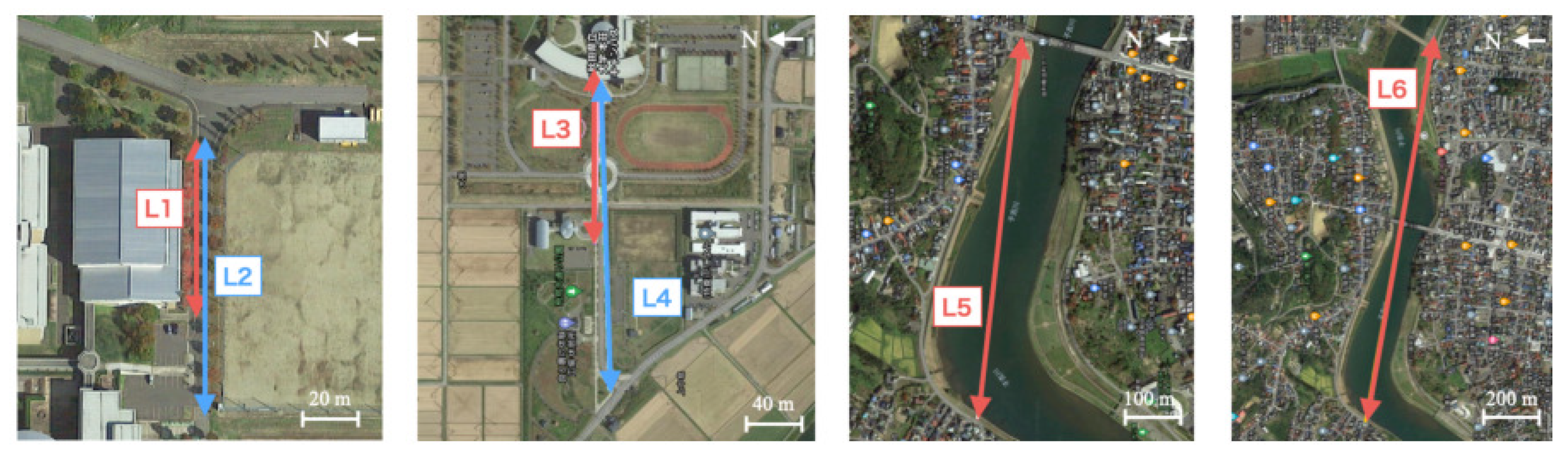
| Parameter | L1 | L2 | L3 | L4 | L5 | L6 |
|---|---|---|---|---|---|---|
| Distance [m] | 60 | 90 | 250 | 490 | 860 | 1360 |
| Data | 20 July 2020 | 30 July 2020 | 17 September 2020 | |||
| Weather | Sunny | Sunny | Sunny | |||
| Atmospheric pressure [hPa] | 1008.8 | 1011.8 | 1007.2 | |||
| Temperature [°C] | 28.5 | 27.4 | 27.9 | |||
| Humidity [%] | 59 | 67 | 63 | |||
| Wind speed [m/s] | 4.9 | 5.4 | 3.3 | |||
| Wind direction | WSW | WSW | SSE | |||
| Index | A [%] | ||
|---|---|---|---|
| L1 | 30 | 30 | 100 |
| L2 | 30 | 30 | 100 |
| L3 | 30 | 30 | 100 |
| L4 | 100 | 100 | 100 |
| L5 | 100 | 98 | 98.0 |
| L6 | 60 | 53 | 88.3 |
| All | 350 | 341 | 97.4 |
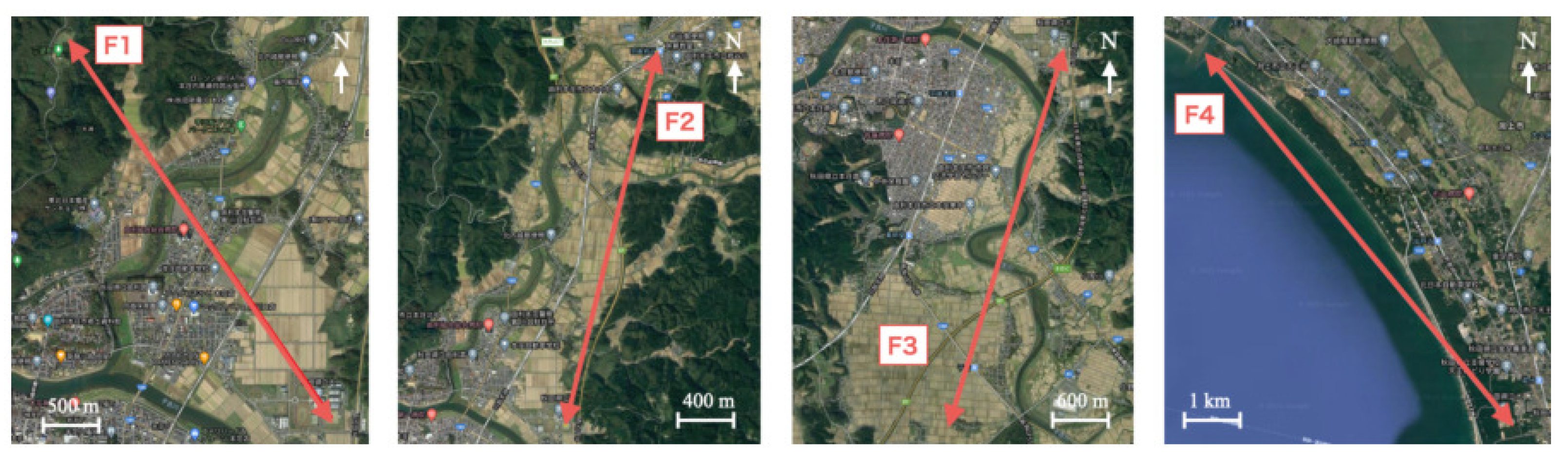
| Parameter | F1 | F2 | F3 | F4 |
|---|---|---|---|---|
| Date | 9 October 2020 | 22 October 2020 | 6 November 2020 | 13 November 2020 |
| Distance [m] | 3500 | 5700 | 5600 | 13,000 |
| Weather | Sunny | Sunny | Sunny | Sunny |
| Atmospheric pressure [hPa] | 1023.4 | 1013.3 | 1018.5 | 1019.4 |
| Temperature [°C] | 18.5 | 20.2 | 16.3 | 13.8 |
| Humidity [%] | 52 | 57 | 75 | 65 |
| Wind speed [m/s] | 2.4 | 5.2 | 3.5 | 2.4 |
| Wind direction | NNE | ESE | S | ESE |
| Flight altitude [m] | ≤150 | ≤150 | ≤150 | ≤150 |
| Index | A [%] | ||
|---|---|---|---|
| F1 | 347 | 309 | 89.0 |
| F2 | 190 | 135 | 71.1 |
| F3 | 390 | 339 | 86.9 |
| F4 | 87 | 82 | 94.3 |
| All | 1014 | 865 | 85.3 |
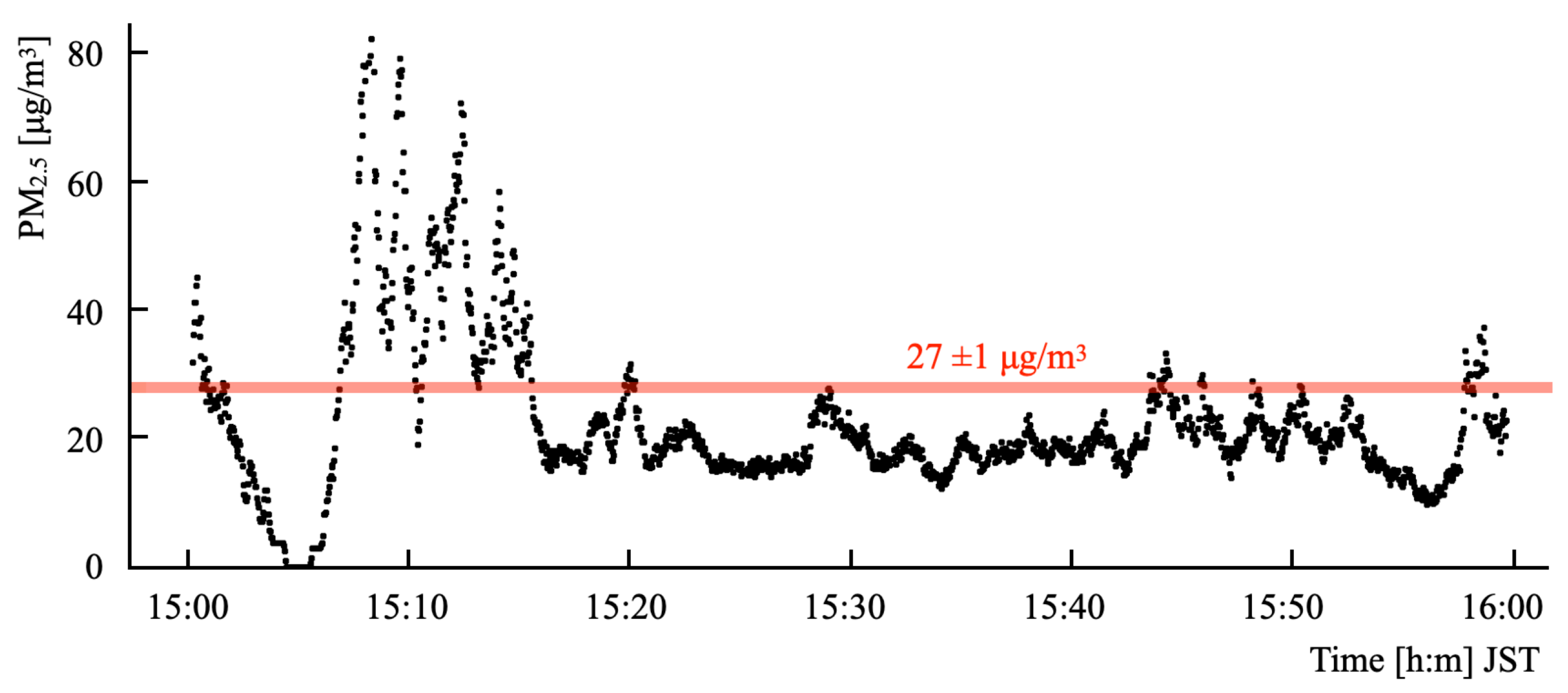
| Parameter | Value |
|---|---|
| Date | 6 November 2020 |
| Time (JST) | 15:00–16:00 |
| Weather | Cloudy |
| Atmospheric pressure | 1019.5 hPa |
| Temperature | 15.3 °C |
| Humidity | 72% |
| Wind speed | 3.3 m/s |
| Wind direction | SSW |
| Precipitation | 0 mm |
| Hours of sunshine | 0 h |
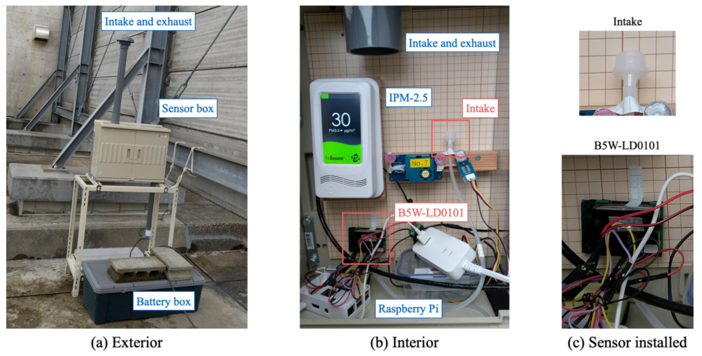
| Parameter | Specification |
|---|---|
| Sensor Type | Light scattering photometer |
| Aerosol concentration range | 5–300 g/m |
| Zero stability | ±10 g/m |
| Time constant | 5 min. trailing average |
| Screen update frequency | 1 Hz |
| Screen resolution | 1 g/m |
| Size | H 162 × W 85 × D 33 mm |
| Weight | 200 g |
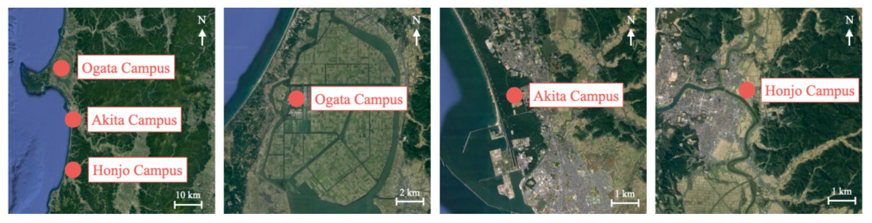
| Parameter | D1 | D2 | D3 |
|---|---|---|---|
| Date | 16 October 2020 | 13 December 2020 | 18 December 2020 |
| Time (JST) | 13:30–14:39 | 15:10–15:53 | 15:17–16:03 |
| Latitude | 39°39′12″ N | 39°80′12″ N | 40°00′64″ N |
| Longitude | 140°04′62″ E | 140°04′62″ E | 139°95′54″ E |
| Site name | Honjo Campus | Akita Campus | Ogata Campus |
| Weather | Sunny | Rain | Sunny |
| Atmospheric pressure [hPa] | 1019.4 | 1018.7 | 1019.6 |
| Temperature [°C] | 14.3 | 11.8 | 12.3 |
| Humidity [%] | 48 | 91 | 67 |
| Wind speed [m/s] | 1.1 | 1.7 | 2.9 |
| Wind direction | ENE | ENE | SE |
| Flight altitude [m] | ≤150 | ≤150 | ≤150 |
| Parameters | Setting Values |
|---|---|
| Learning iteration [epoch] | 100 |
| Batch size | 2 |
| Validation rate | 0.2 |
| Number of hidden layers | 50 |
| Optimization algorithms | RMSprop |
| L | 30, 10, and 5 |
| Dataset | L | Training [g/m] | Test [g/m] |
|---|---|---|---|
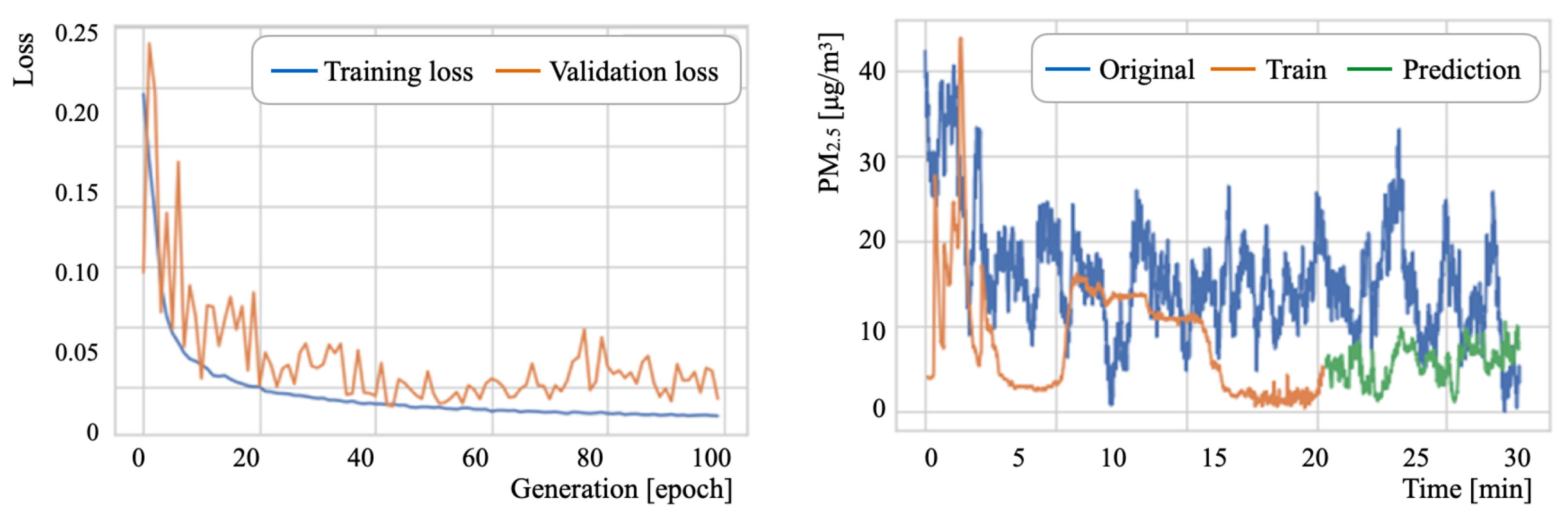
| D1 | 30 | 3.06 | 3.99 |
| 10 | 1.80 | 3.73 | |
| 5 | 2.01 | 2.60 | |
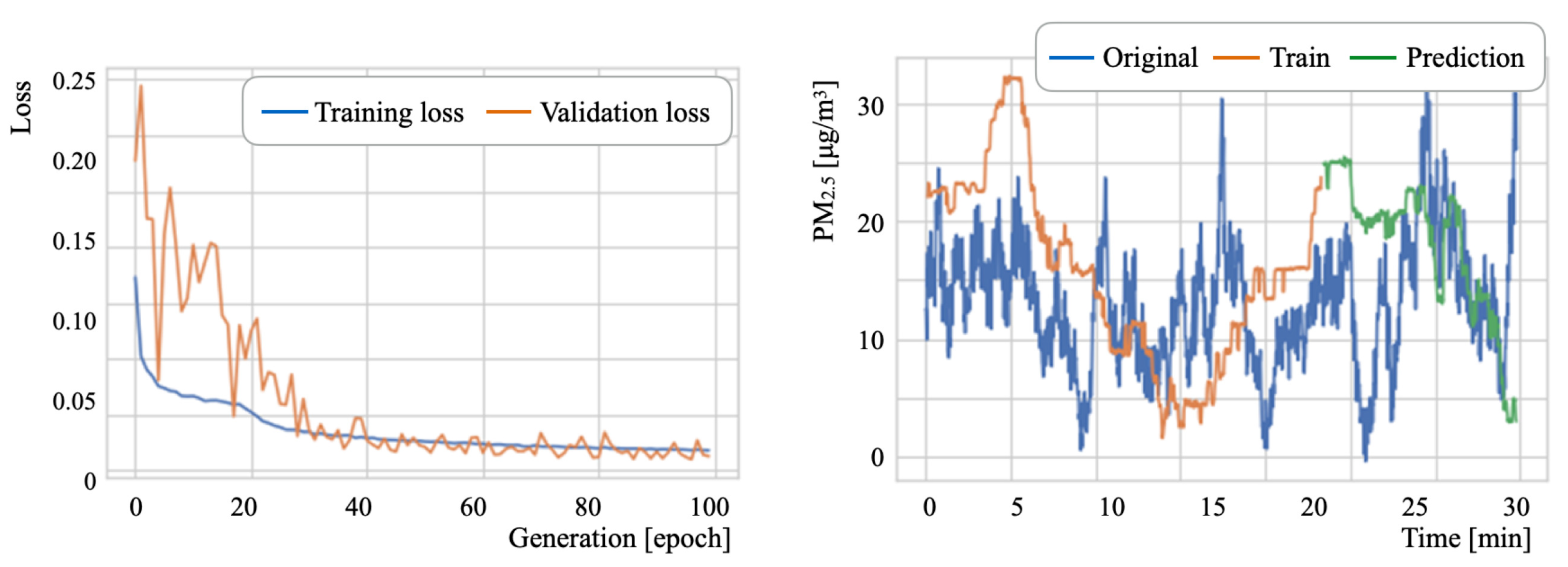
| D2 | 30 | 3.07 | 9.57 |
| 10 | 1.97 | 4.48 | |
| 5 | 1.59 | 1.97 | |
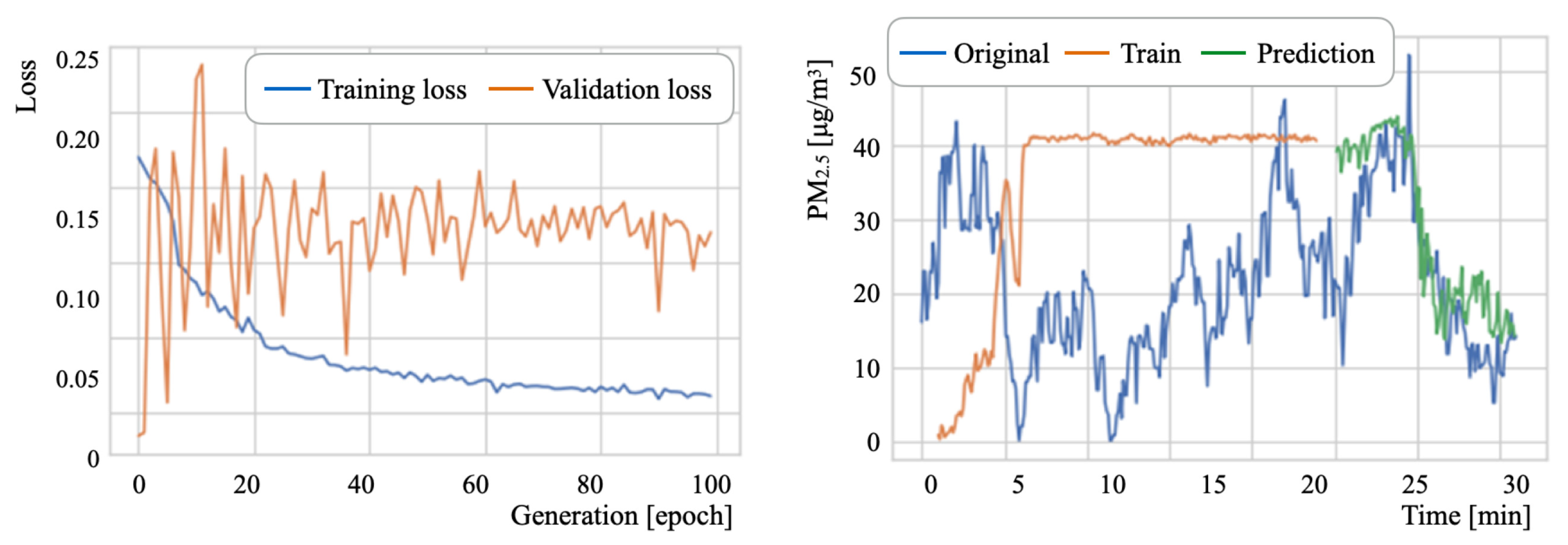
| D3 | 30 | 6.01 | 14.74 |
| 10 | 5.84 | 16.23 | |
| 5 | 6.12 | 19.07 |
Publisher’s Note: MDPI stays neutral with regard to jurisdictional claims in published maps and institutional affiliations. |
© 2021 by the authors. Licensee MDPI, Basel, Switzerland. This article is an open access article distributed under the terms and conditions of the Creative Commons Attribution (CC BY) license (https://creativecommons.org/licenses/by/4.0/).
Share and Cite
Madokoro, H.; Kiguchi, O.; Nagayoshi, T.; Chiba, T.; Inoue, M.; Chiyonobu, S.; Nix, S.; Woo, H.; Sato, K. Development of Drone-Mounted Multiple Sensing System with Advanced Mobility for In Situ Atmospheric Measurement: A Case Study Focusing on PM2.5 Local Distribution. Sensors 2021, 21, 4881. https://doi.org/10.3390/s21144881
Madokoro H, Kiguchi O, Nagayoshi T, Chiba T, Inoue M, Chiyonobu S, Nix S, Woo H, Sato K. Development of Drone-Mounted Multiple Sensing System with Advanced Mobility for In Situ Atmospheric Measurement: A Case Study Focusing on PM2.5 Local Distribution. Sensors. 2021; 21(14):4881. https://doi.org/10.3390/s21144881
Chicago/Turabian StyleMadokoro, Hirokazu, Osamu Kiguchi, Takeshi Nagayoshi, Takashi Chiba, Makoto Inoue, Shun Chiyonobu, Stephanie Nix, Hanwool Woo, and Kazuhito Sato. 2021. "Development of Drone-Mounted Multiple Sensing System with Advanced Mobility for In Situ Atmospheric Measurement: A Case Study Focusing on PM2.5 Local Distribution" Sensors 21, no. 14: 4881. https://doi.org/10.3390/s21144881
APA StyleMadokoro, H., Kiguchi, O., Nagayoshi, T., Chiba, T., Inoue, M., Chiyonobu, S., Nix, S., Woo, H., & Sato, K. (2021). Development of Drone-Mounted Multiple Sensing System with Advanced Mobility for In Situ Atmospheric Measurement: A Case Study Focusing on PM2.5 Local Distribution. Sensors, 21(14), 4881. https://doi.org/10.3390/s21144881