
Precision Temperature Control for the Laser Gyro Inertial Navigation System in Long-Endurance Marine Navigation

Abstract
1. Introduction
2. Materials and Methods
2.1. Theoretical Analysis on Inertial Navigation System and Accelerometer
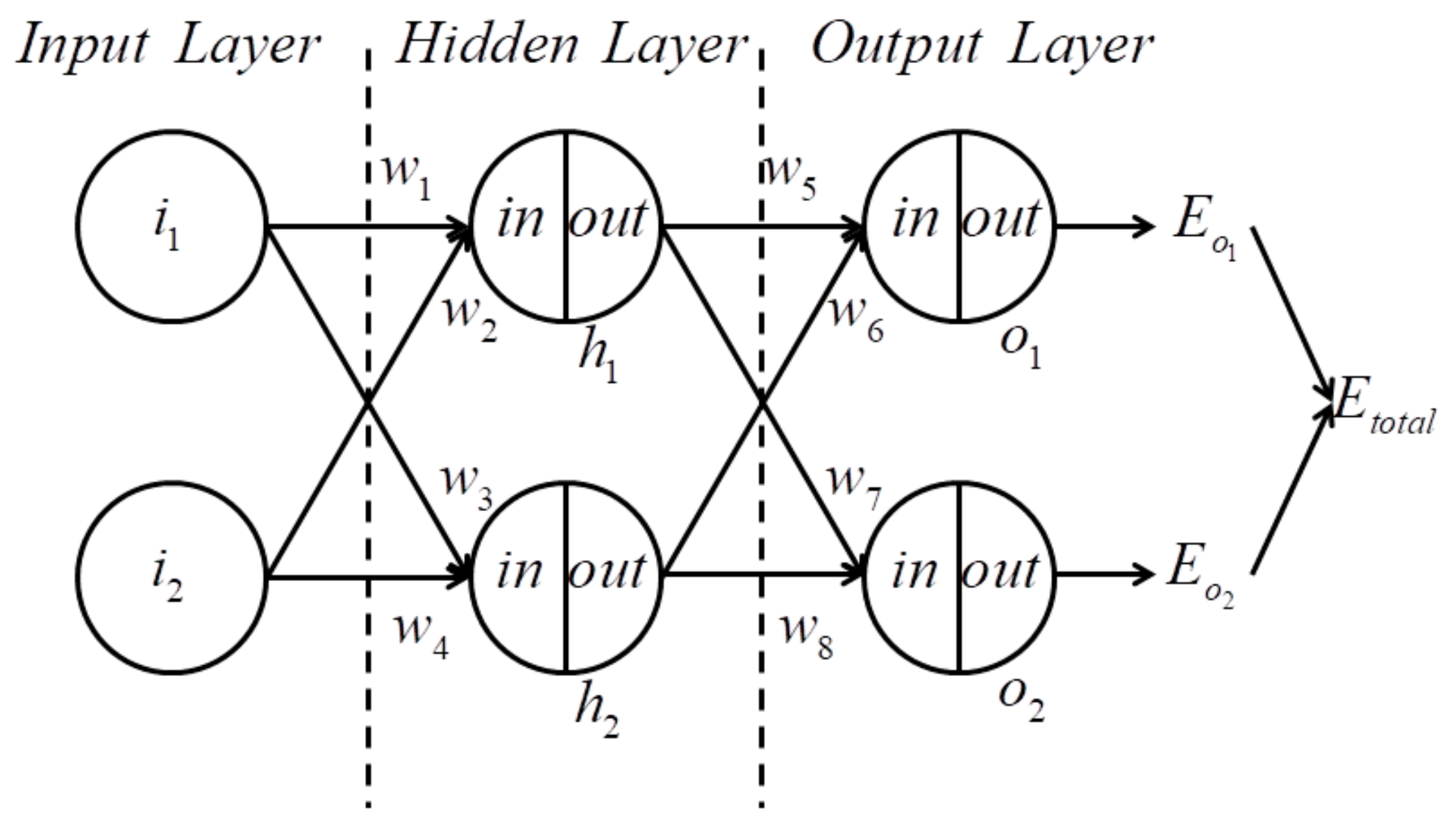
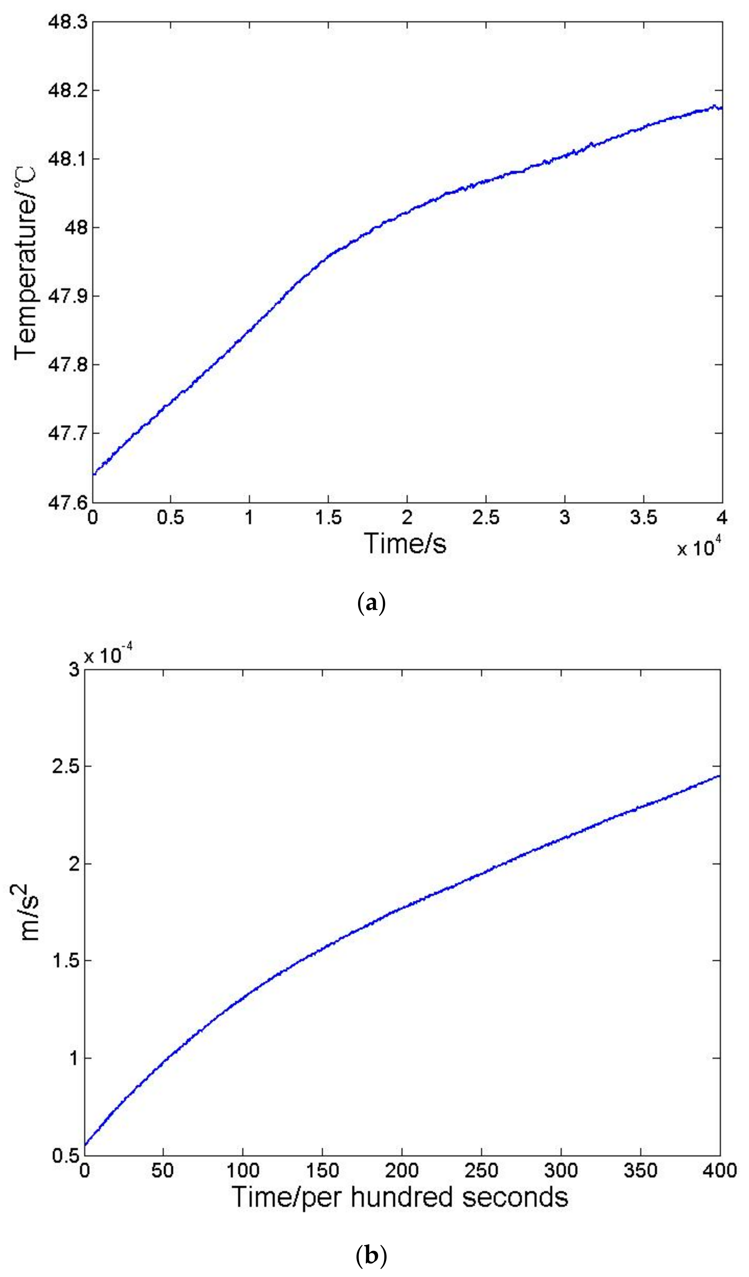
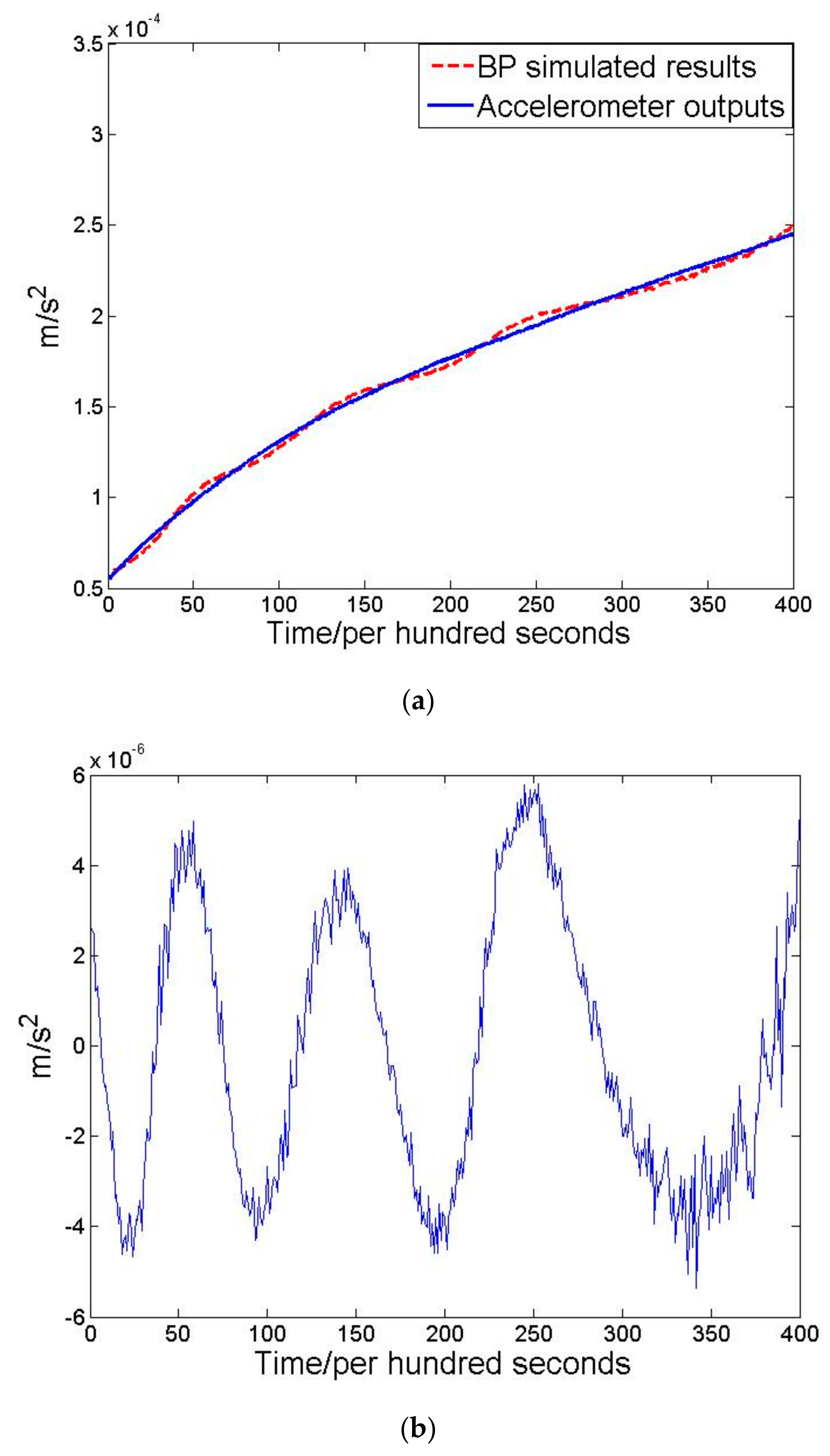
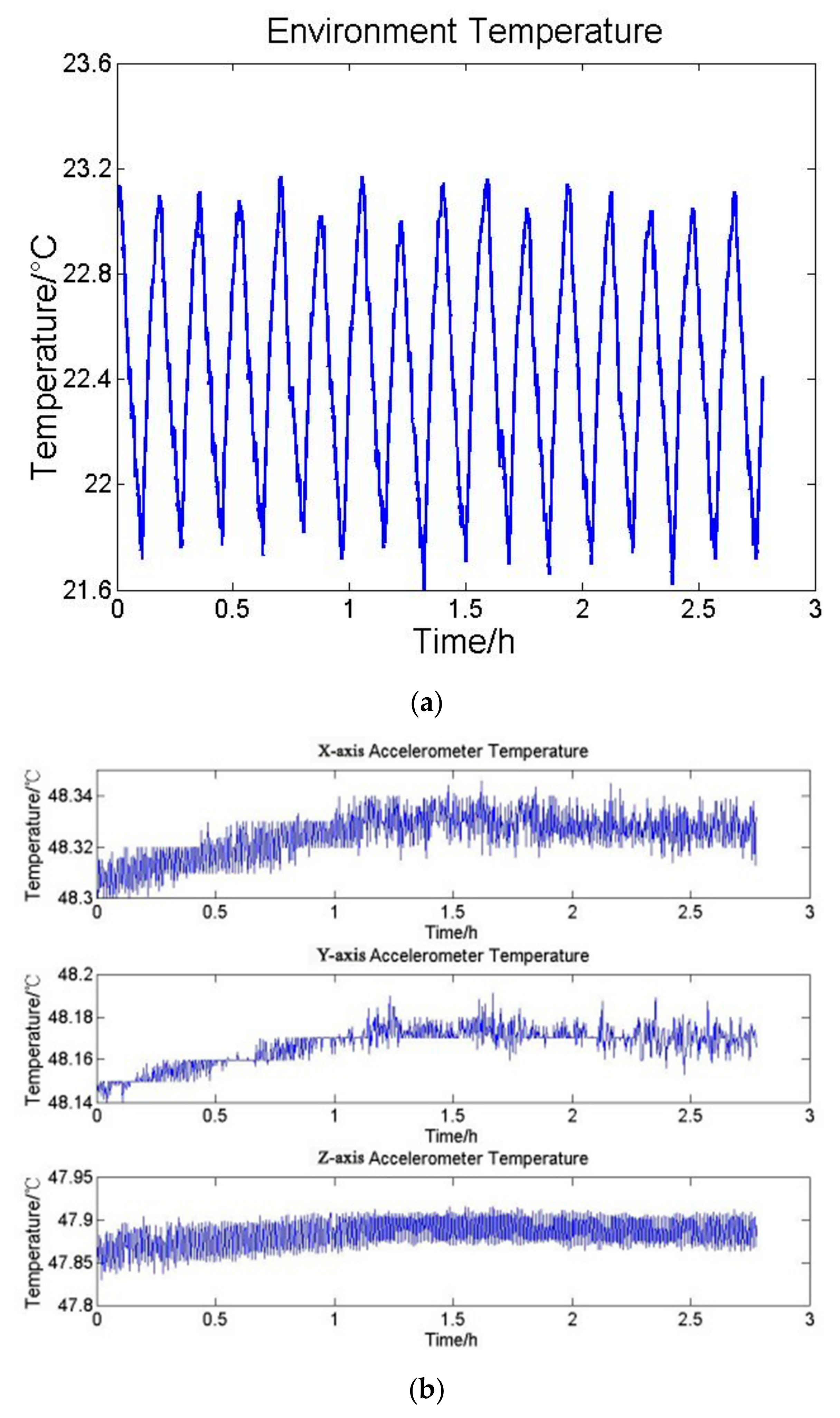
2.2. Verification on Theoretical Analysis Based on BP-NN Algorithm
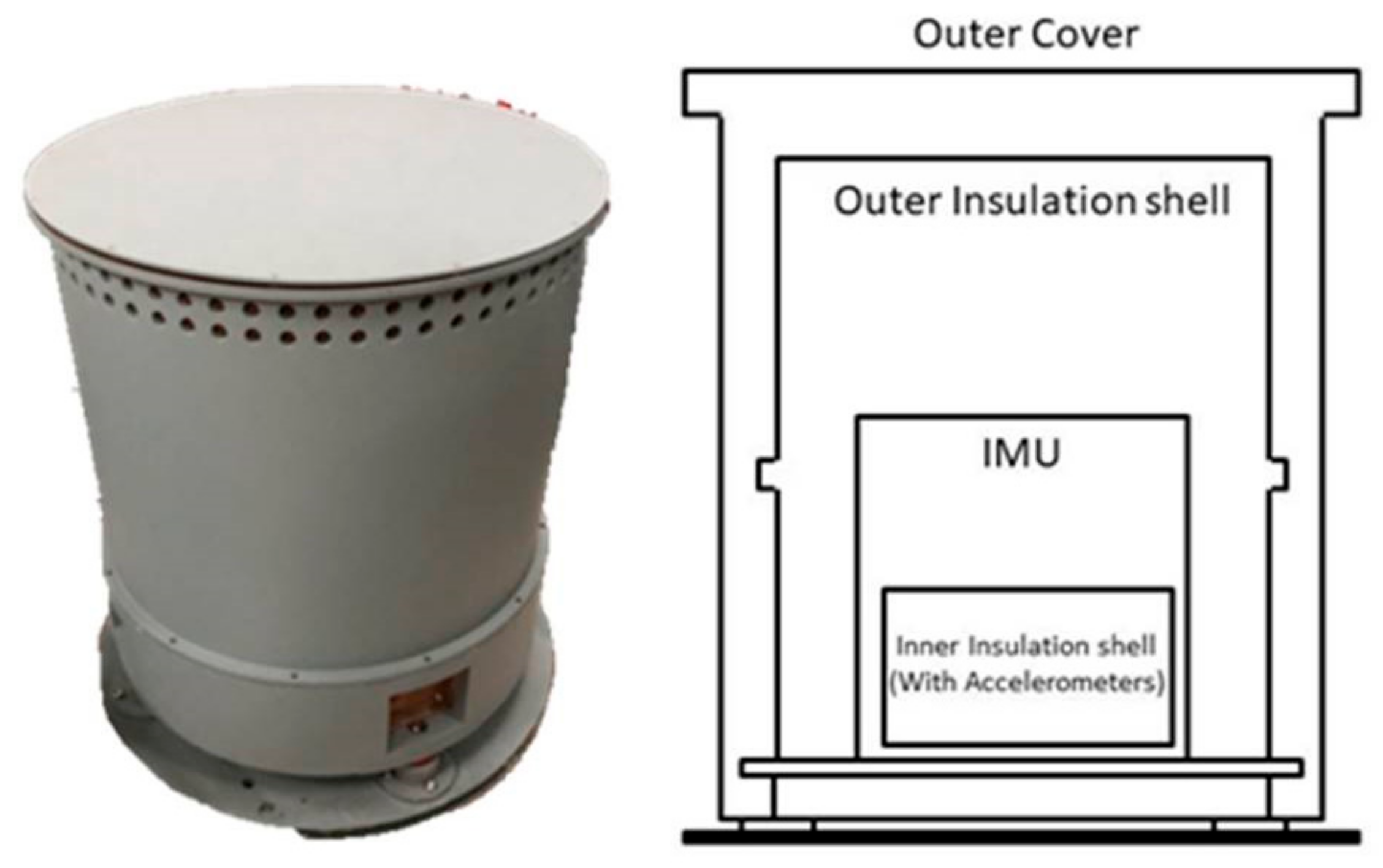
2.3. Profile of Precise Temperature Control System
3. Results
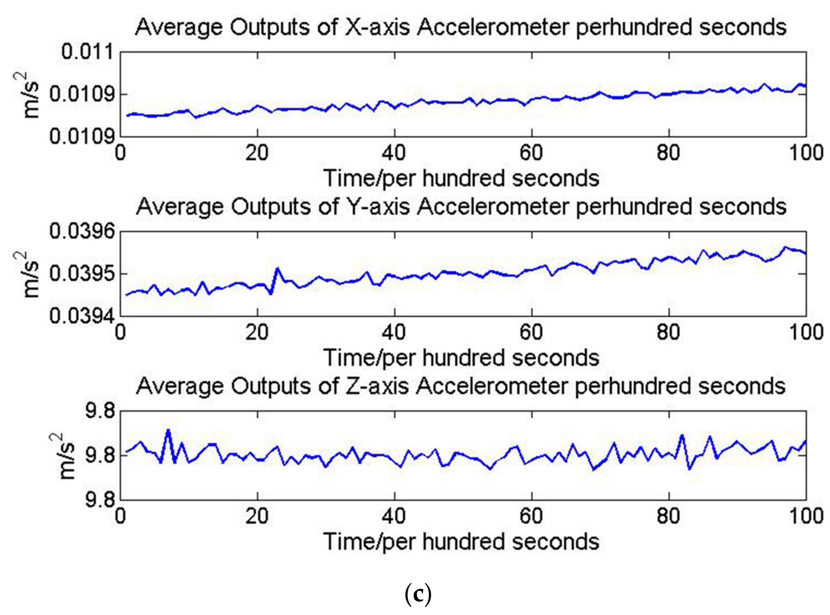
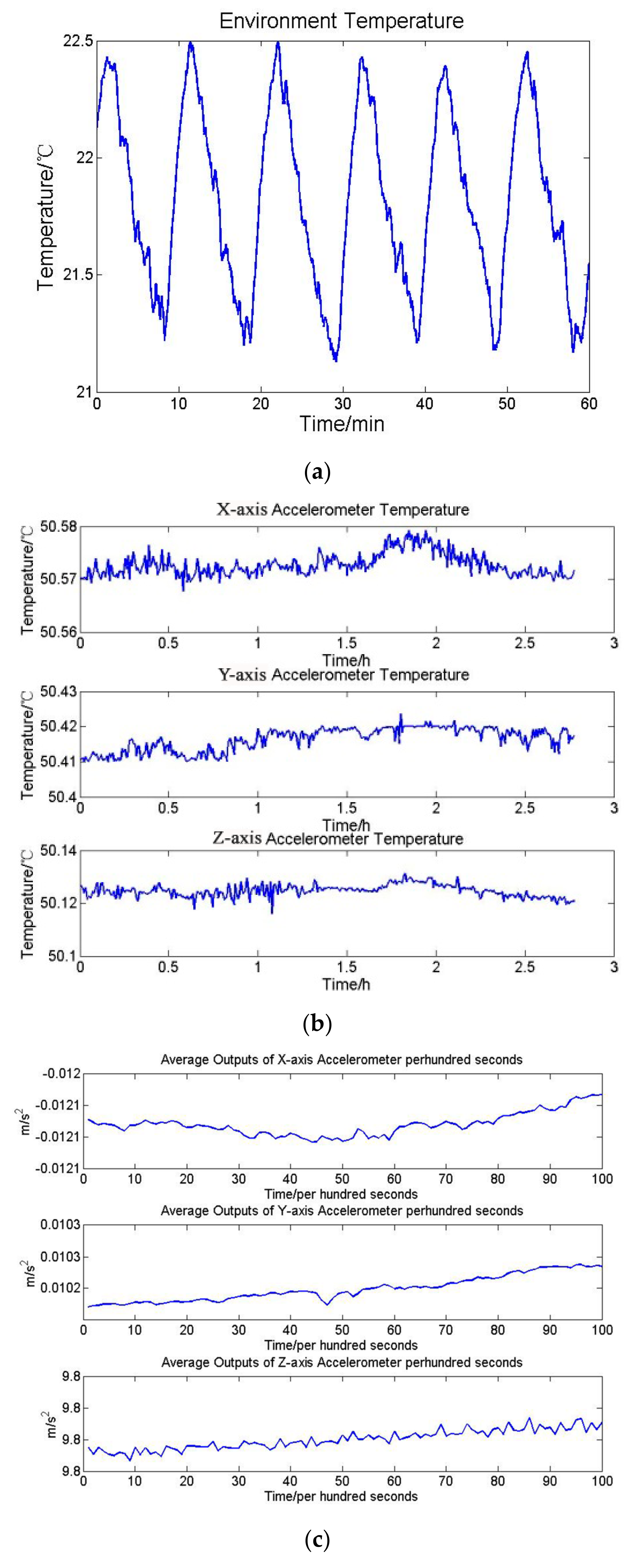
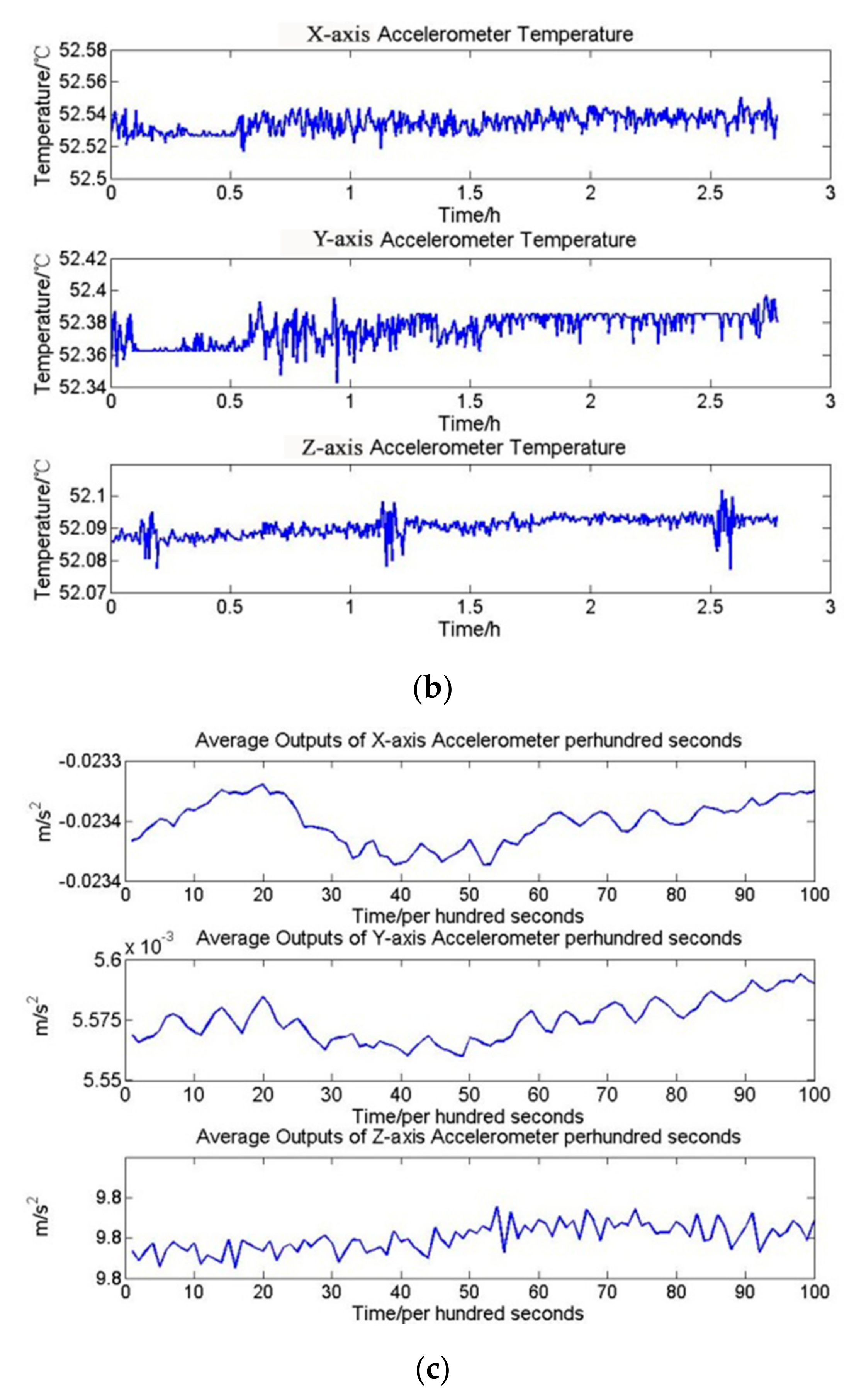
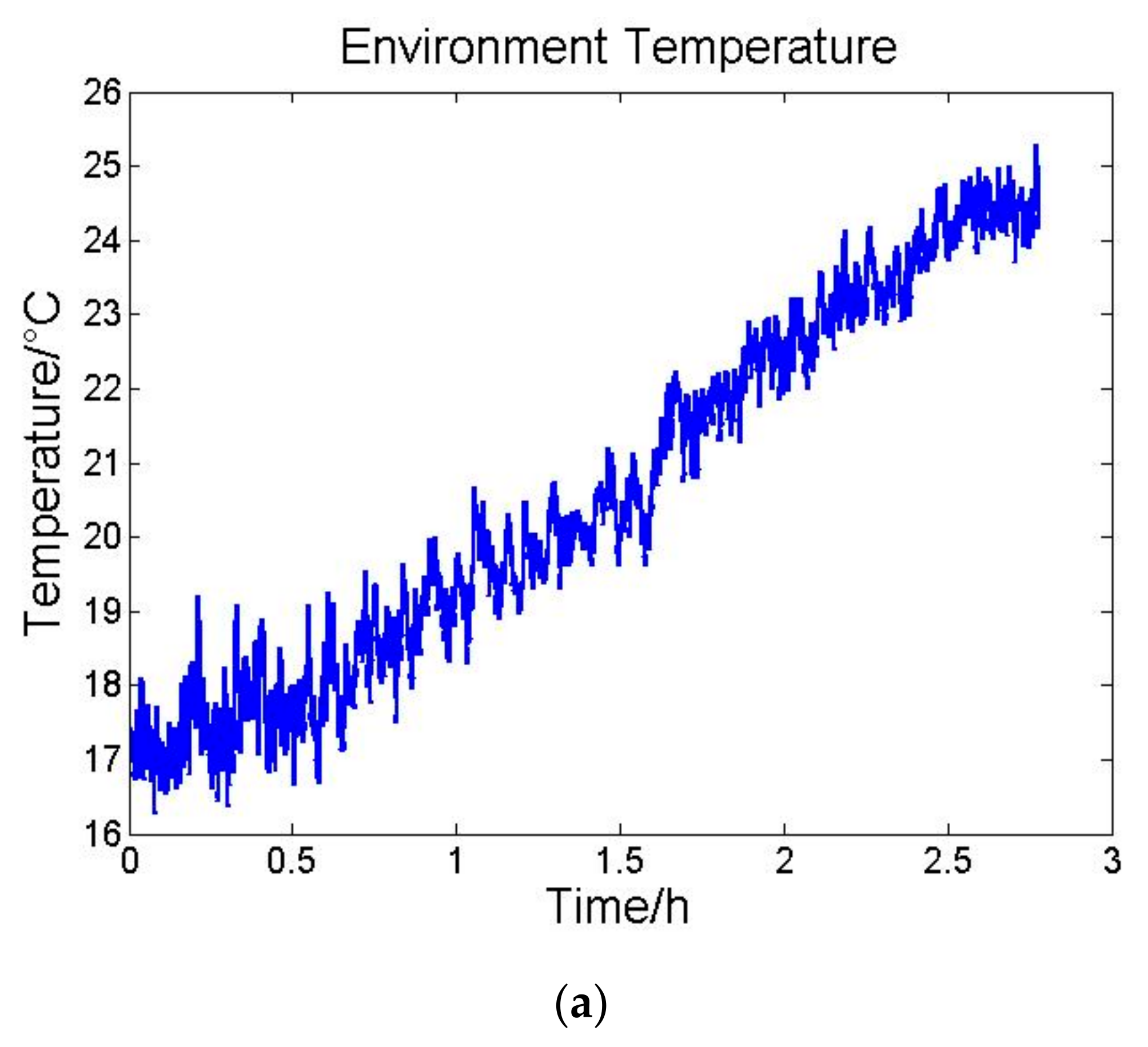
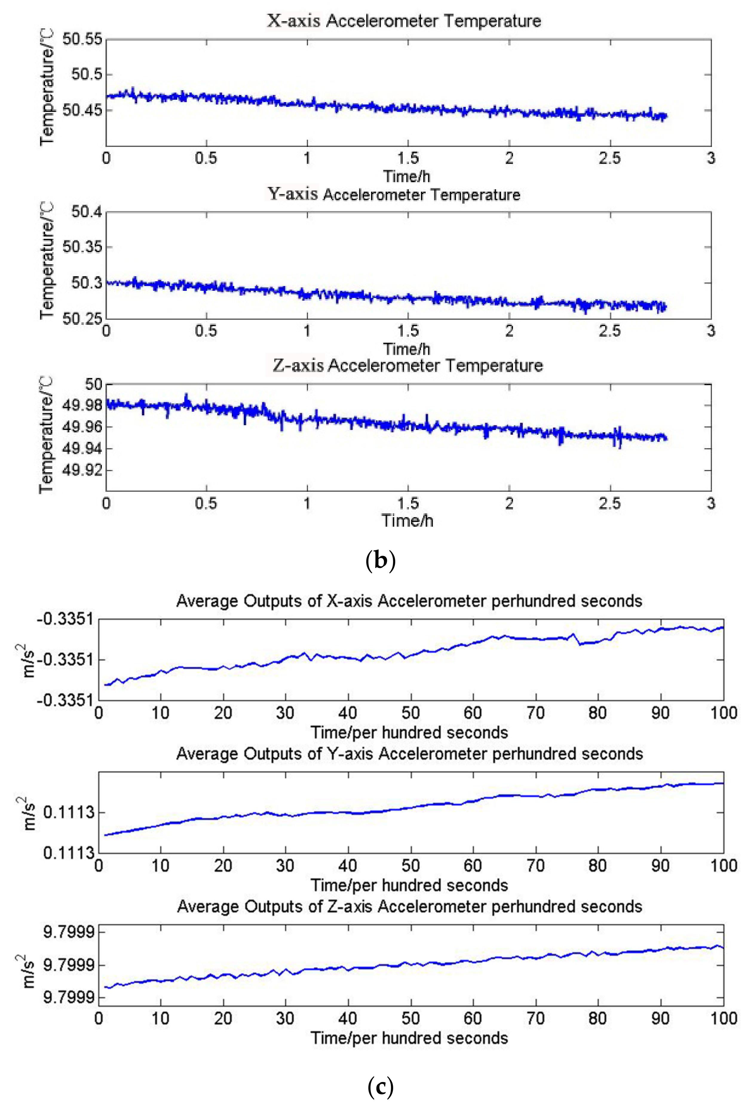
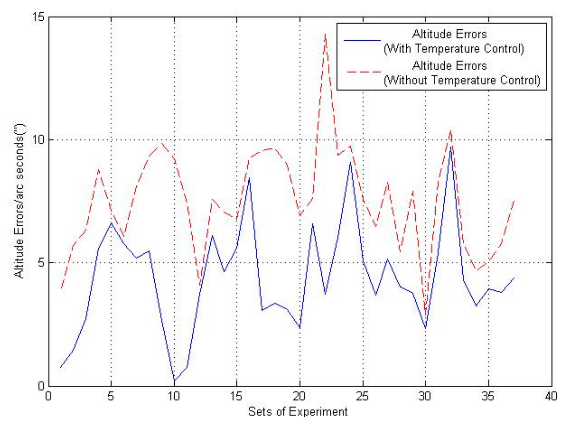
3.1. Contrast Experiments on Precise Temperature Control System
3.2. Performance Experiments on Precise Temperature Control System
4. Discussion
5. Conclusions
Author Contributions
Funding
Institutional Review Board Statement
Informed Consent Statement
Data Availability Statement
Conflicts of Interest
References
- Baird, W.H. An introduction to inertial navigation. Am. J. Phys. 2009, 77, 844–847. [Google Scholar] [CrossRef][Green Version]
- Heekwon, N.O.; Kee, C. Enhancement of GPS/INS Navigation System Observability Using a Triaxial Magnetometer. Trans. Jpn. Soc. Aeronaut. Space Sci. 2019, 62, 125–136. [Google Scholar]
- Alaluev, R.V.; Ivanov, Y.V.; Malyutin, D.M. High-precision algorithmic compensation of temperature instability of accelerometer’s scaling factor. Autom. Remote Control 2011, 72, 853–860. [Google Scholar] [CrossRef]
- Simav, M.; Becker, D.; Yildiz, H.; Hoss, M. Impact of temperature stabilization on the strapdown airborne gravimetry: A case study in Central Turkey. J. Geod. 2020, 94, 41. [Google Scholar] [CrossRef]
- Takumi, N.; Masaya, K.; Yorinao, I. A new system for detection of thermoluminescence and delayed luminescence from photosynthetic apparatus with precise temperature control. Spectrosc. Int. J. 2002, 277, 27765–27771. [Google Scholar]
- Daigo, Y.; Watanabe, T.; Ishiguro, A.; Ishii, S.; Kushibe, M.; Moriyama, Y. Impact of precise temperature control for 4H-SiC epitaxy on large diameter wafers. In Proceedings of the 2020 International Symposium on Semiconductor Manufacturing (ISSM), Tokyo, Japan, 15–16 December 2020. [Google Scholar]
- Lei, Z.; Xie, D.; Mbogba, M.K.; Chen, Z.; Tian, C.; Xu, L.; Zhao, G. A microfluidic platform with cell-scale precise temperature control for simultaneous investigation of the osmotic responses of multiple oocytes. Lab Chip 2019, 19, 1929–1940. [Google Scholar] [CrossRef] [PubMed]
- Linzon, Y.; Rutkowska, K.A.; Malomed, B.A.; Morandotti, R. Magnetooptical control of light collapse in bulk Kerr media. Phys. Rev. Lett. 2009, 103, 053902. [Google Scholar] [CrossRef] [PubMed]
- Lloyd-Hart, M. System for precise temperature sensing and thermal control of borosilicate honeycomb mirrors during polishing and testing. Int. Soc. Opt. Photonics 1990. [Google Scholar] [CrossRef]
- Oliver, J.W. An Introduction to Inertial Navigation; UCAM-CL-TR-696; University of Cambridge: London, UK, 2007; 15p. [Google Scholar]
- Titterton, D.H.; Weston, J. Strapdown Inertial Navigation Technology; Institution of Electrical Engineers: London, UK, 2004; 594p. [Google Scholar]
- Barulina, M.A.; Dzhashitov, V.E.; Pankratov, V.M. Mathematical model of a micromechanical accelerometer with temperature influences, dynamic effects, and the thermoelastic stress-strain state taken into account. Gyroscopy Navig. 2010, 1, 52–61. [Google Scholar] [CrossRef]
- Hong, W.S.; Lee, K.S.; Paik, B.S.; Han, J.Y.; Son, S.H. The compensation method for thermal bias of ring laser gyro. In Proceedings of the LEOS 2008 - 21st Annual Meeting of the IEEE Lasers and Electro-Optics Society, Newport Beach, CA, USA, 9–13 November 2008; pp. 723–724. [Google Scholar]
- Dzhashitov, V.E.; Pankratov, V.M.; Golikov, A.V.; Nikolaev, S.G.; Kolevatov, A.P.; Plonikov, A.D.; Koffer, K.V. Hierarchical thermal models of FOG-based strapdown inertial navigation system. Gyroscopy Navig. 2014, 5, 162–173. [Google Scholar] [CrossRef]
- Gao, J.M.; Zhang, K.B.; Chen, F.B.; Yang, H.B. Temperature characteristics and error compensation for quartz flexible accelerometer. Int. J. Autom. Comput. 2015, 12, 540–550. [Google Scholar] [CrossRef][Green Version]
- Dong, X.; Huang, Q.; Xu, W.; Tang, B.; Yang, S.; Zhu, J.; En, Y. Research on temperature characteristic of parasitic capacitance in MEMS capacitive accelerometer. Sens. Actuators A Phys. 2019, 285, 581–587. [Google Scholar] [CrossRef]
- Li, J.L. Study and implementation of the precise temperature control used in airborne gravimetry. In Proceedings of the 2010 8th World Congress on Intelligent Control and Automation, Jinan, China, 7–9 July 2010; pp. 2064–2068. [Google Scholar]
- Lee, K.I.; Takao, H.; Sawada, K. A three-axis accelerometer for high temperatures with low temperature dependence using a constant temperature control of SOI piezoresistors. In Proceedings of the The Sixteenth Annual International Conference on Micro Electro Mechanical Systems, Kyoto, Japan, 23 January 2003; pp. 478–481. [Google Scholar]
- Liu, D.B.; Hu, P.H.; Shen, Y. Research on High-Accuracy Temperature Control for Airborne/Marine Gravimeter Based on Inertial Stabilized Platform. Navig. Position. Timing 2017, 4, 29–35. [Google Scholar]
- Li, J.L.; Zhang, K.D.; Zhang, Q. A performance analysis and precise temperature control of accelerometers for airborne gravimetry. Int. Conf. Electron. Meas. Instrum. 2009, 1, 35–38. [Google Scholar] [CrossRef]
- Cao, J.L.; Wang, M.H.; Cai, S.Q.; Zhang, K.D.; Wu, M.P. Optimized Design of the SGA-WZ Strapdown Airborne Gravimeter Temperature Control System. Sensors 2015, 15, 29984–29996. [Google Scholar] [CrossRef] [PubMed]
- Wang, S.; Zhu, W.; Shen, Y.; Ren, J.; Gu, H.; Wei, X. Temperature compensation for MEMS resonant accelerometer based on genetic algorithm optimized backpropagation neural network. Sens. Actuators A Phys. 2020, 316, 112393. [Google Scholar] [CrossRef]
- Thimm, G.; Moerland, P.; Fiesler, E. The Interchangeability of Learning Rate and Gain in Backpropagation Neural Networks. Neural Comput. 2014, 8, 451–460. [Google Scholar] [CrossRef] [PubMed]
- García-Valdovinos, L.G.; Fonseca-Navarro, F.; Aizpuru-Zinkunegi, J.; Salgado-Jiménez, T.; Gómez-Espinosa, A.; Cruz-Ledesma, J.A. Neuro-Sliding Control for Underwater ROV’s Subject to Unknown Disturbances. Sensors 2019, 19, 2943. [Google Scholar] [CrossRef] [PubMed]
- Zhu, M.; Pang, L.; Xiao, Z.; Shen, C. Temperature Drift Compensation for High-G MEMS Accelerometer Based on RBF NN Improved Method. Appl. Sci. 2019, 9, 695. [Google Scholar] [CrossRef]


| Time (s) | Standard Deviation of Temperature (°C) | Mean Square Deviation Per Hundred Seconds of Accelerometer Outputs (×10−5 m/s2) |
|---|---|---|
| 1–10,000 | 0.0602 | 13.2301 |
| 10,001–20,000 | 0.0513 | 10.3651 |
| 20,001–30,000 | 0.0227 | 3.7755 |
| 30,001–40,000 | 0.0216 | 3.2664 |
| Time(s) | Standard Deviation of Temperature (°C) | Mean Square Deviation Per Hundred Seconds of Accelerometer Outputs (×10−5 m/s2) |
|---|---|---|
| 1–10,000 | 0.02 | 3.1290 |
| 10,001–20,000 | 0.015 | 1.7060 |
| 20,001–30,000 | 0.01 | 0.9339 |
| 30,001–40,000 | 0.005 | 0.5892 |
| X-Axis Accelerometer | Y-Axis Accelerometer | Z-Axis Accelerometer | |
|---|---|---|---|
| Deviation of Temperature | 0.0568 °C | 0.0542 °C | 0.0503 °C |
| Mean square deviation per hundred seconds of Outputs | 5.2985 × 10⁻⁵ m/s2 | 5.9909 × 10⁻⁵ m/s2 | 5.0517 × 10⁻⁵ m/s2 |
| X-Axis Accelerometer | Y-Axis Accelerometer | Z-Axis Accelerometer | |
|---|---|---|---|
| Deviation of Temperature | 0.0074 °C | 0.0080 °C | 0.0067 °C |
| Mean square deviation per hundred seconds of Outputs | 0.7306 × 10⁻⁵ m/s2 | 0.8045 × 10⁻⁵ m/s2 | 0.6151 × 10⁻⁵ m/s2 |
| X-Axis Accelerometer | Y-Axis Accelerometer | Z-Axis Accelerometer | |
|---|---|---|---|
| Deviation of Temperature | 0.0079 °C | 0.0085 °C | 0.0070 °C |
| Mean square deviation per hundred seconds of Outputs | 0.7807 × 10⁻⁵ m/s2 | 0.8758 × 10⁻⁵ m/s2 | 0.6931 × 10⁻⁵ m/s2 |
| X-Axis Accelerometer | Y-Axis Accelerometer | Z-Axis Accelerometer | |
|---|---|---|---|
| Deviation of Temperature | 0.0087 °C | 0.0091 °C | 0.0081 °C |
| Mean square deviation per hundred seconds of Outputs | 0.8026 × 10⁻⁵ m/s2 | 0.9190 × 10⁻⁵ m/s2 | 0.7480 × 10⁻⁵ m/s2 |
| Sets of Experiment | Altitude Error/ Arc Seconds (With Temperature Control) | Altitude Error/ Arc Seconds (Without Temperature Control) | Percetange Improvements |
|---|---|---|---|
| 1 | 0.75 | 3.83 | 80.41% |
| 2 | 1.45 | 5.69 | 74.51% |
| 3 | 2.74 | 6.33 | 56.71% |
| 4 | 5.59 | 8.79 | 36.40% |
| 5 | 6.63 | 7.14 | 7.14% |
| 6 | 5.76 | 6.07 | 5.10% |
| 7 | 5.19 | 8.07 | 35.68% |
| 8 | 5.50 | 9.32 | 40.98% |
| 9 | 2.66 | 9.83 | 72.93% |
| 10 | 0.21 | 9.22 | 97.72% |
| 11 | 0.74 | 7.43 | 90.04% |
| 12 | 3.74 | 4.08 | 8.33% |
| 13 | 6.11 | 7.59 | 19.49% |
| 14 | 4.64 | 7.07 | 34.37% |
| 15 | 5.59 | 6.75 | 17.18% |
| 16 | 8.45 | 9.27 | 8.84% |
| 17 | 3.08 | 9.56 | 67.78% |
| 18 | 3.35 | 9.65 | 65.28% |
| 19 | 3.11 | 8.95 | 65.25% |
| 20 | 2.38 | 6.93 | 65.65% |
| 21 | 6.58 | 7.62 | 13.64% |
| 22 | 3.71 | 14.30 | 74.05% |
| 23 | 6.02 | 9.36 | 35.68% |
| 24 | 9.06 | 9.72 | 6.79% |
| 25 | 5.08 | 7.56 | 32.80% |
| 26 | 3.69 | 6.48 | 43.05% |
| 27 | 5.15 | 8.28 | 37.80% |
| 28 | 4.00 | 5.43 | 26.33% |
| 29 | 3.76 | 7.92 | 52.52% |
| 30 | 2.34 | 2.88 | 18.75% |
| 31 | 5.41 | 8.28 | 34.66% |
| 32 | 9.69 | 10.4 | 6.82% |
| 33 | 4.32 | 5.76 | 25% |
| 34 | 3.24 | 4.68 | 30.76% |
| 35 | 3.96 | 5.04 | 21.42% |
| 36 | 3.78 | 5.76 | 34.37% |
| Mean Value | 4.37 | 7.53 | 41.97% |
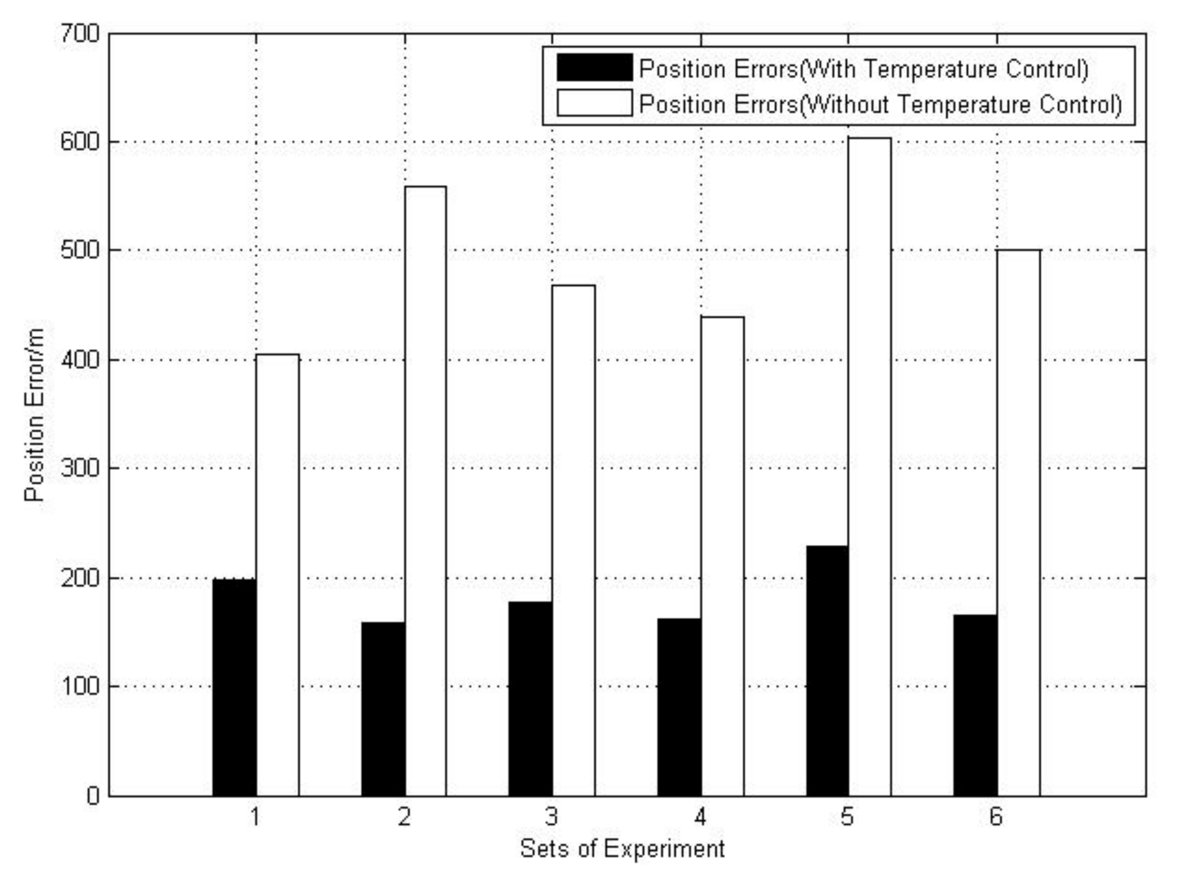
| Sets of Experiments | Position Error/m (With Temperature Control) | Position Error/m (Without Temperature Control) | Percentage Improvement |
|---|---|---|---|
| 1 | 196.87 | 404.82 | 51.36% |
| 2 | 158.35 | 559.42 | 71.69% |
| 3 | 177.00 | 468.58 | 62.22% |
| 4 | 161.89 | 439.61 | 63.17% |
| 5 | 228.87 | 603.10 | 62.051% |
| 6 | 165.68 | 501.40 | 66.95% |
| Mean Value | 181.44 | 496.16 | 62.91% |
Publisher’s Note: MDPI stays neutral with regard to jurisdictional claims in published maps and institutional affiliations. |
© 2021 by the authors. Licensee MDPI, Basel, Switzerland. This article is an open access article distributed under the terms and conditions of the Creative Commons Attribution (CC BY) license (https://creativecommons.org/licenses/by/4.0/).
Share and Cite
Xiong, Z.; Wei, G.; Gao, C.; Long, X. Precision Temperature Control for the Laser Gyro Inertial Navigation System in Long-Endurance Marine Navigation. Sensors 2021, 21, 4119. https://doi.org/10.3390/s21124119
Xiong Z, Wei G, Gao C, Long X. Precision Temperature Control for the Laser Gyro Inertial Navigation System in Long-Endurance Marine Navigation. Sensors. 2021; 21(12):4119. https://doi.org/10.3390/s21124119
Chicago/Turabian StyleXiong, Zhenyu, Guo Wei, Chunfeng Gao, and Xingwu Long. 2021. "Precision Temperature Control for the Laser Gyro Inertial Navigation System in Long-Endurance Marine Navigation" Sensors 21, no. 12: 4119. https://doi.org/10.3390/s21124119
APA StyleXiong, Z., Wei, G., Gao, C., & Long, X. (2021). Precision Temperature Control for the Laser Gyro Inertial Navigation System in Long-Endurance Marine Navigation. Sensors, 21(12), 4119. https://doi.org/10.3390/s21124119