
Multi-Sensor and Decision-Level Fusion-Based Structural Damage Detection Using a One-Dimensional Convolutional Neural Network


Abstract
1. Introduction
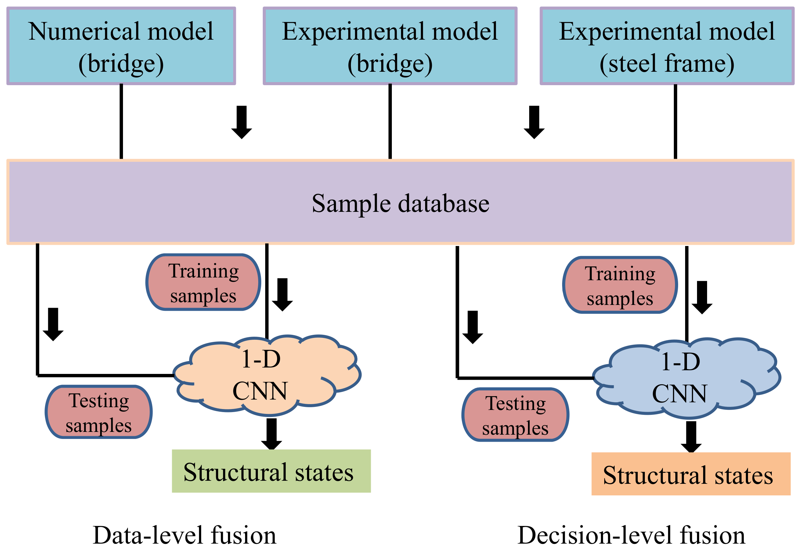
2. Materials and Methods
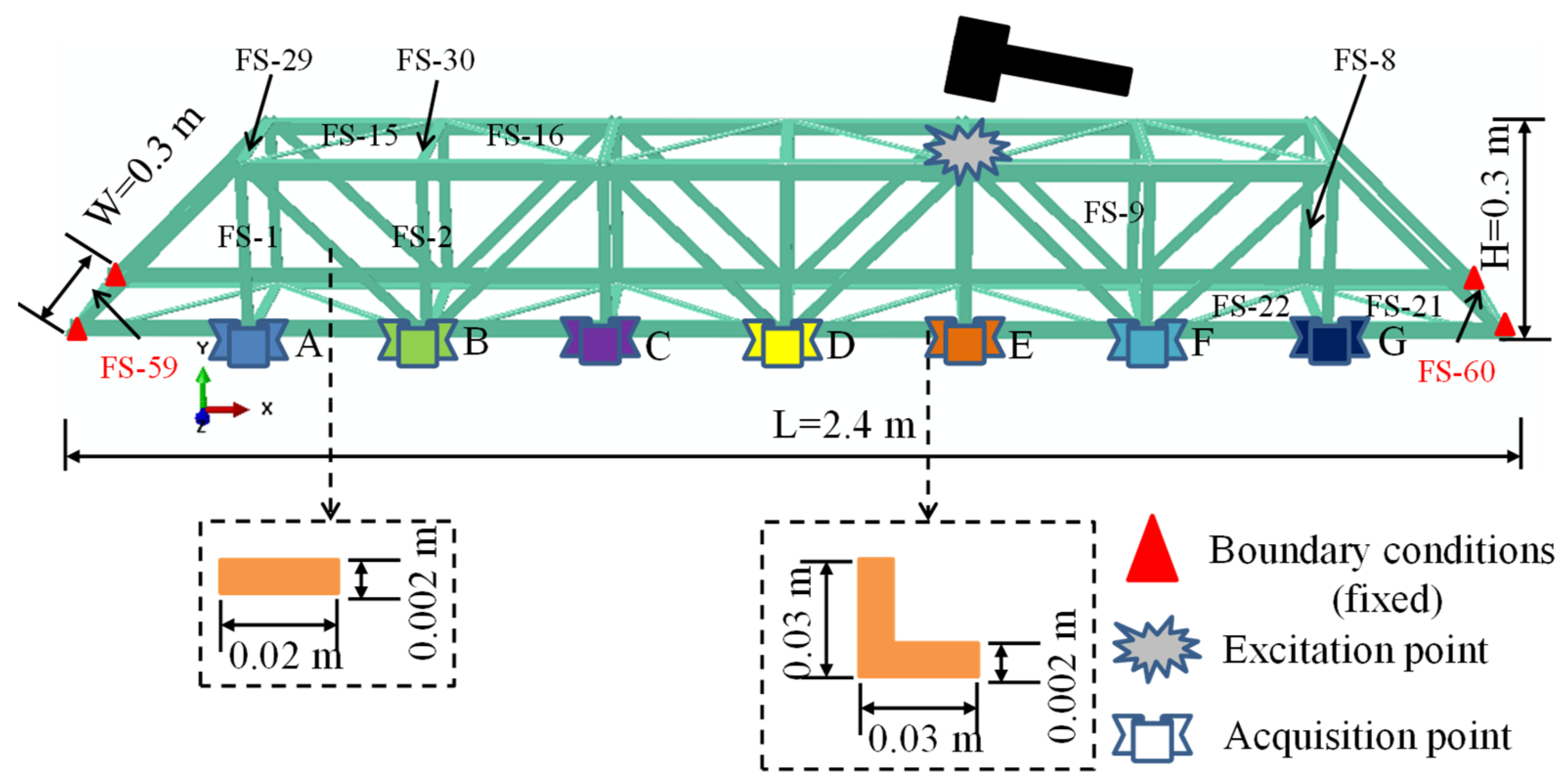
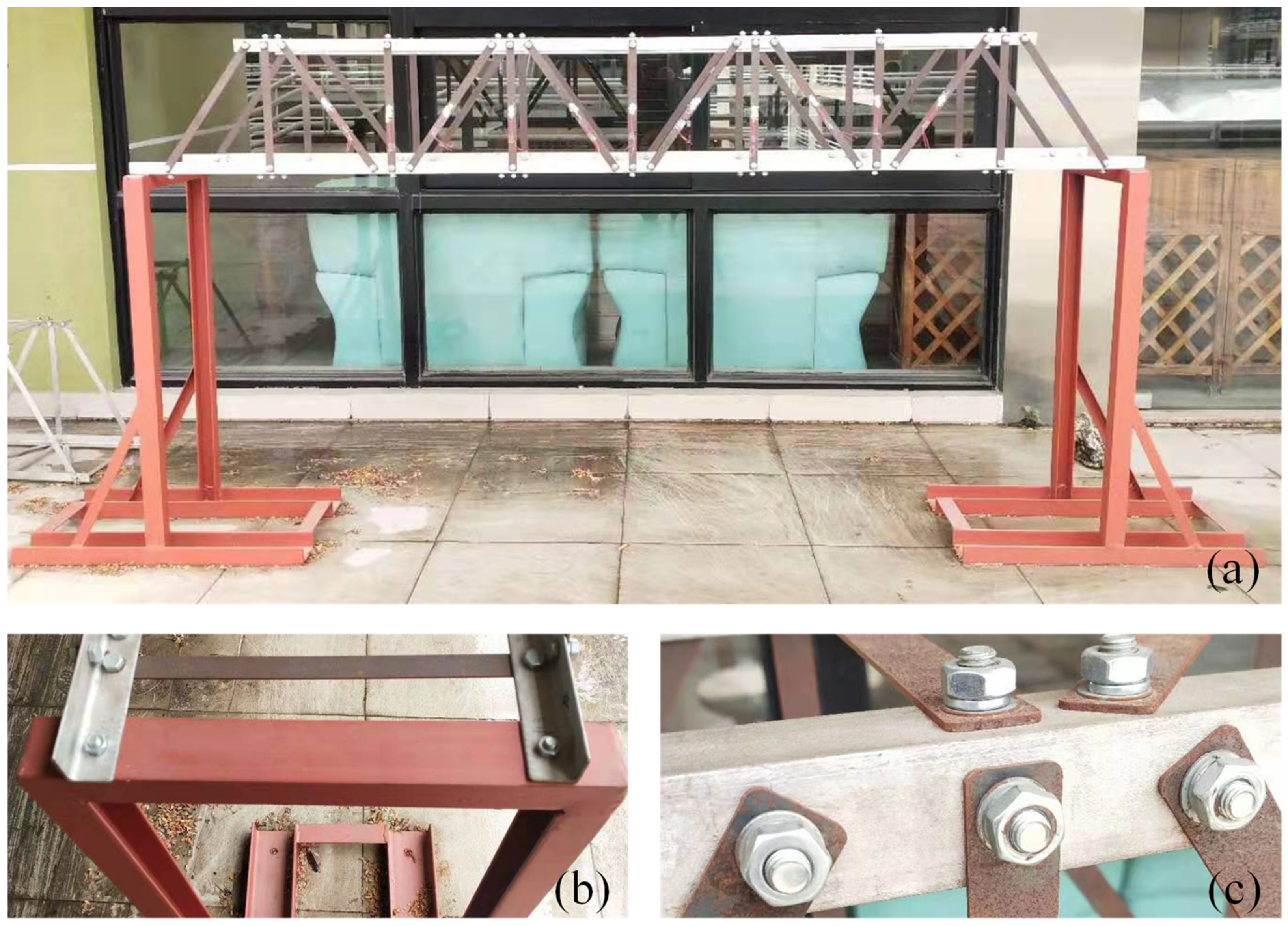
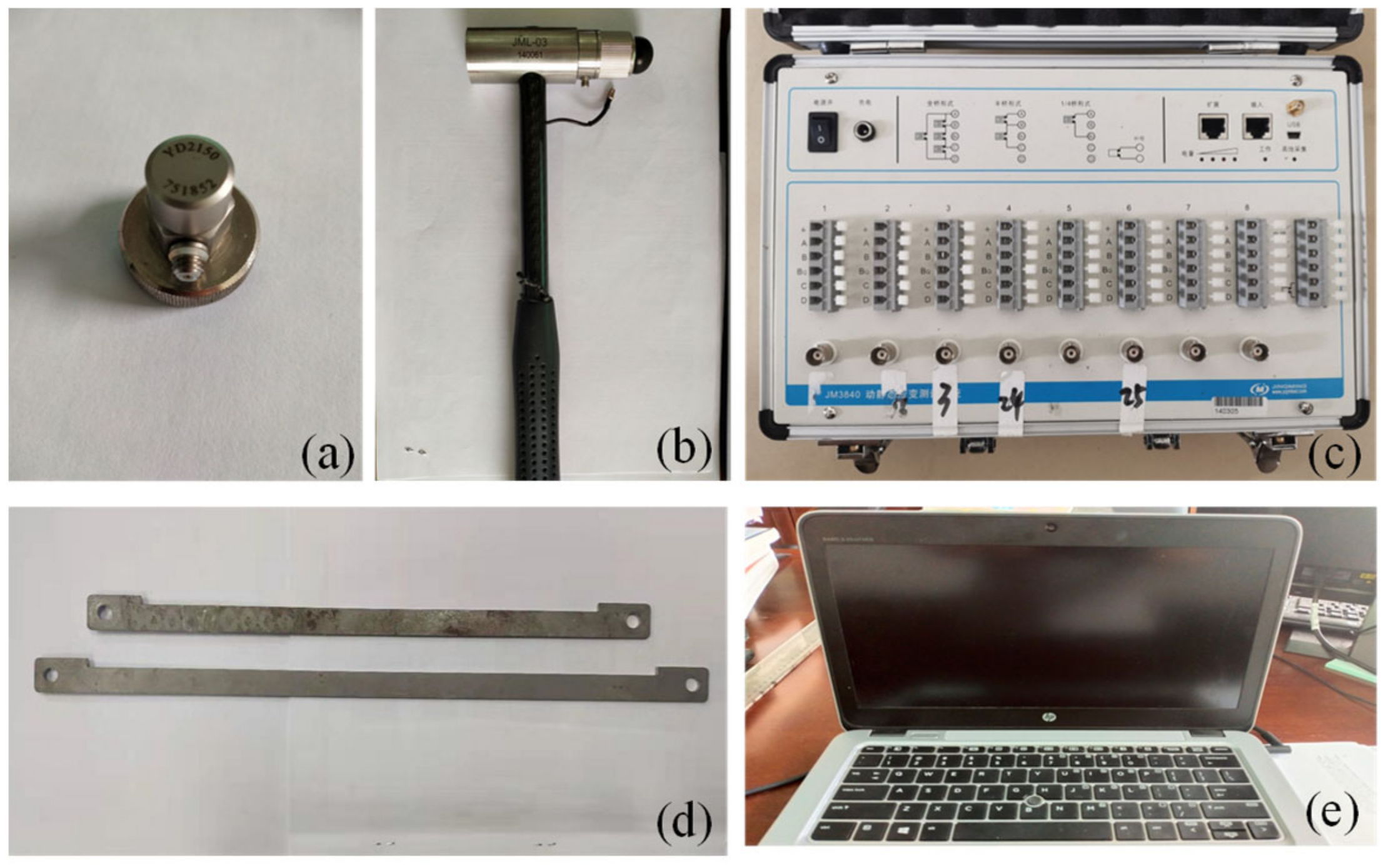
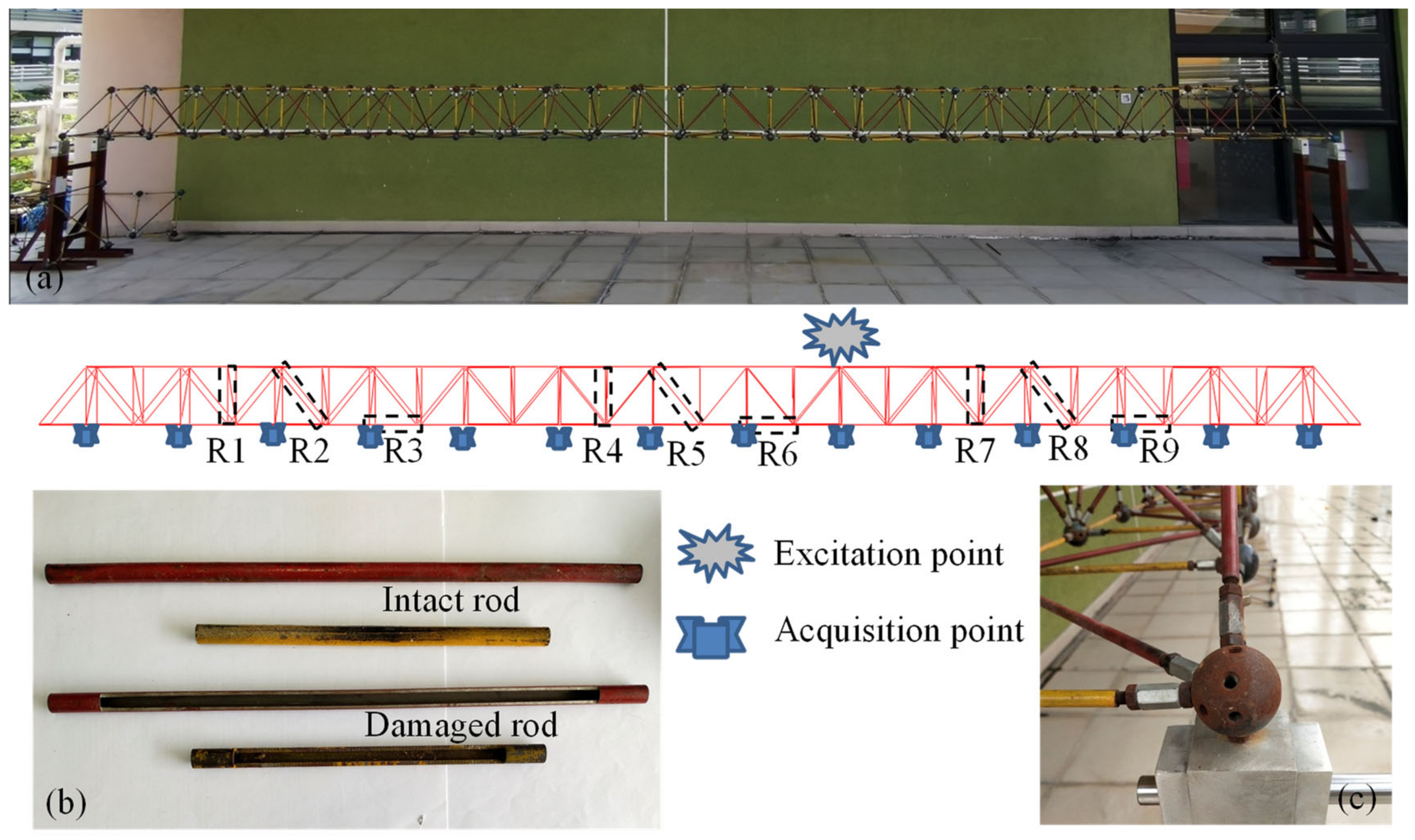
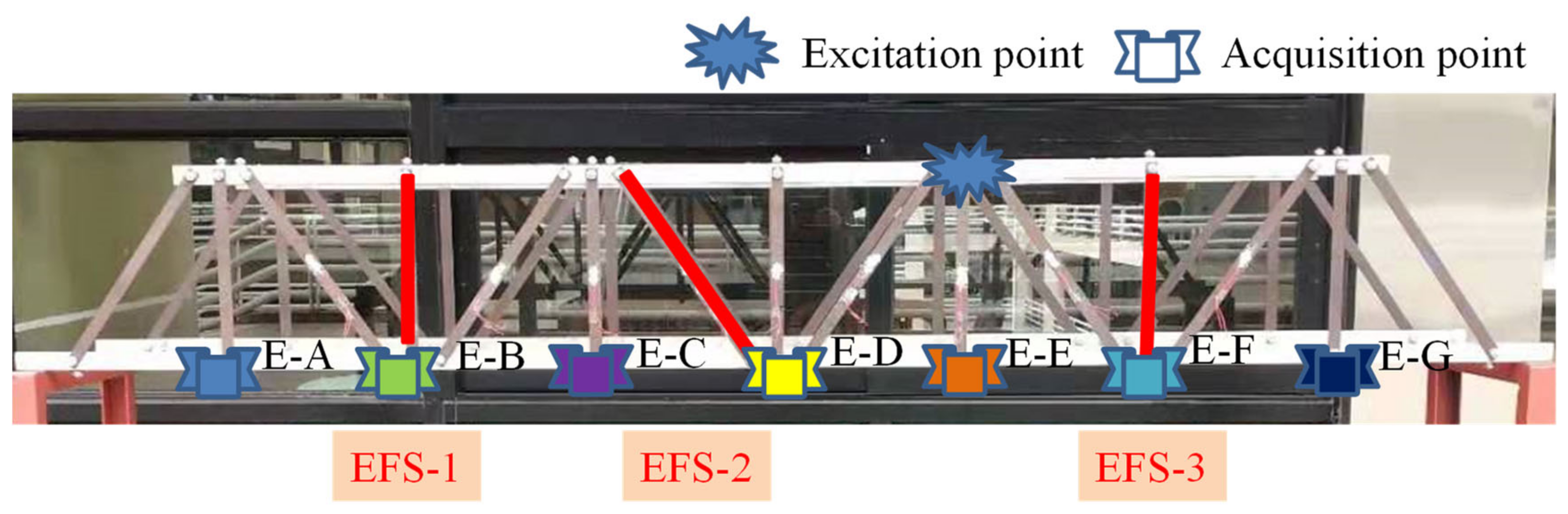
2.1. Numerical and Experimental Models
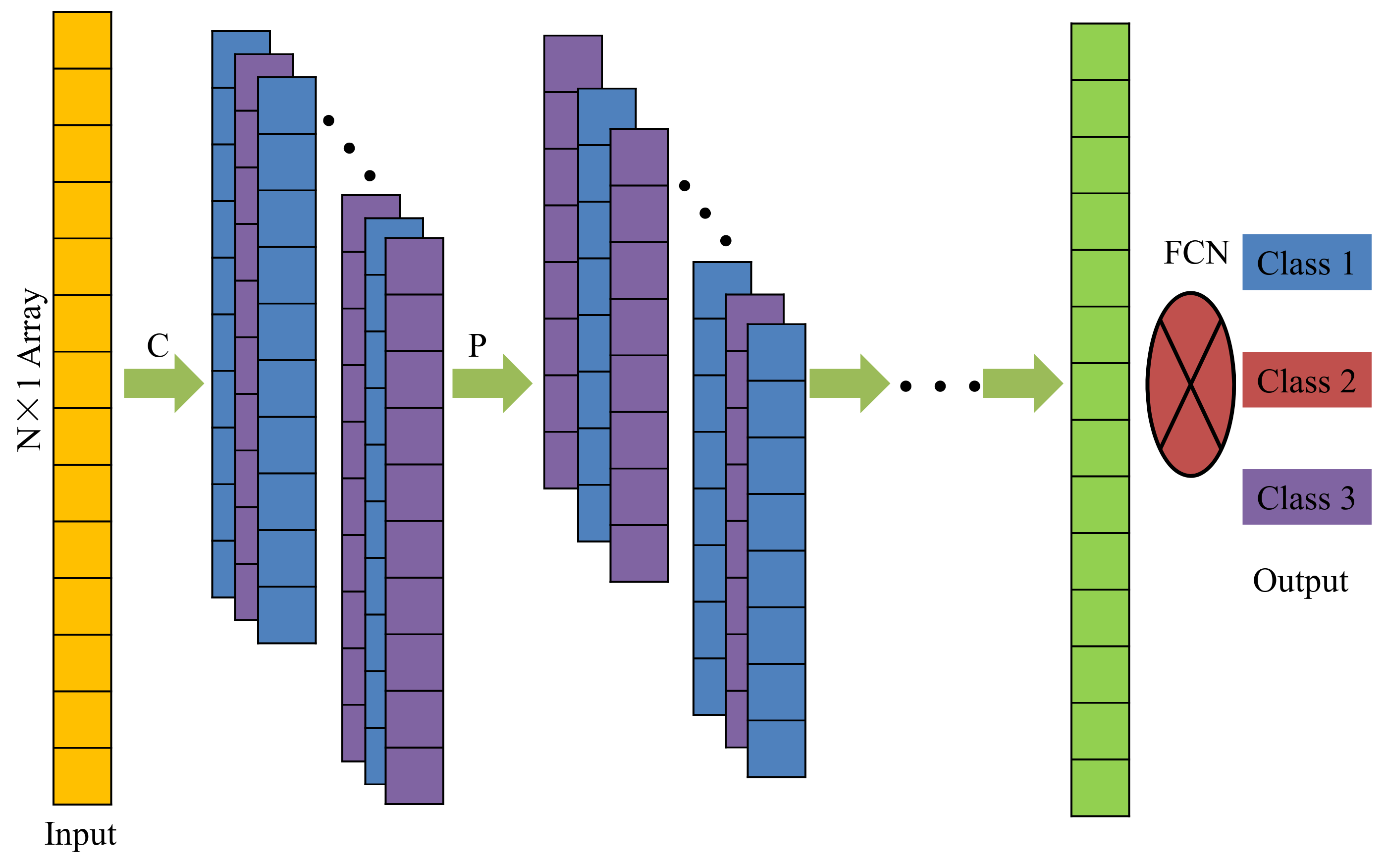
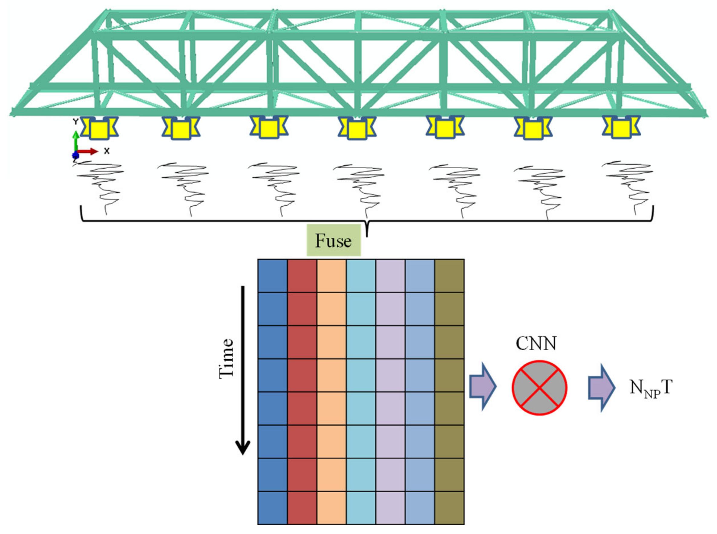
2.2. 1-D Convolution Neural Network
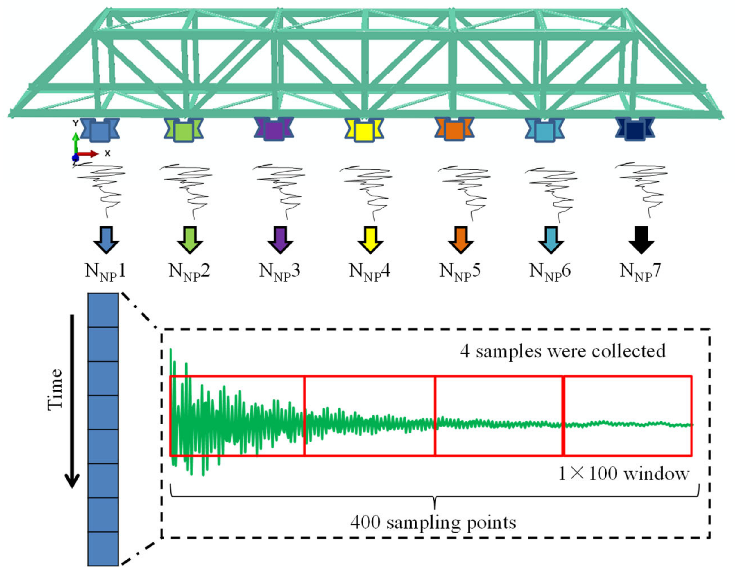
2.3. Structural Damage Detection
3. Results and Discussion
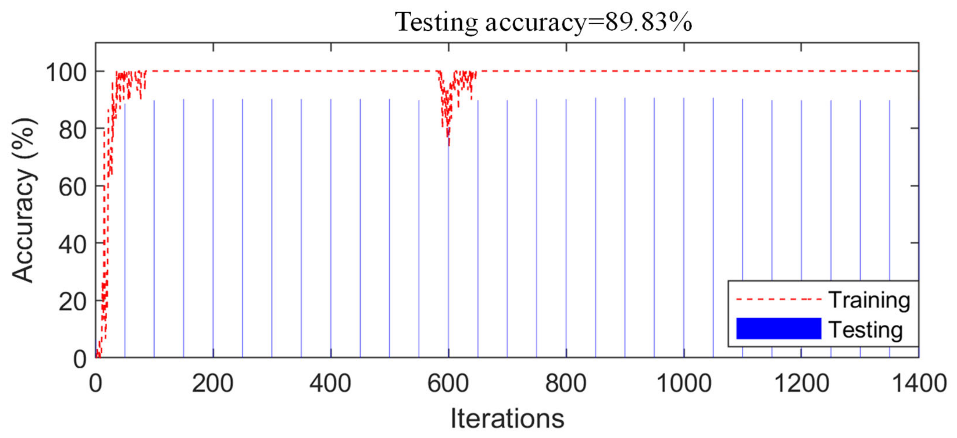
3.1. Detection Results of the Numerical Model
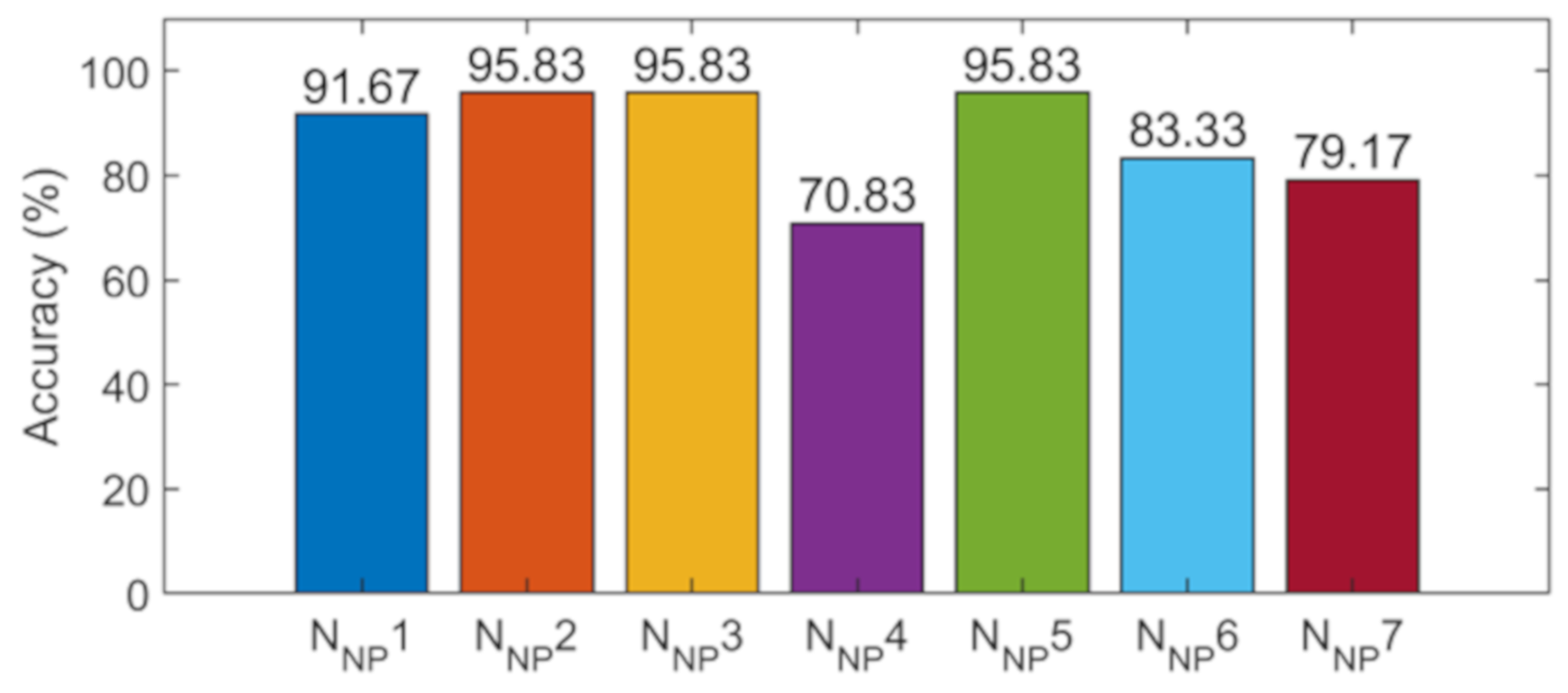
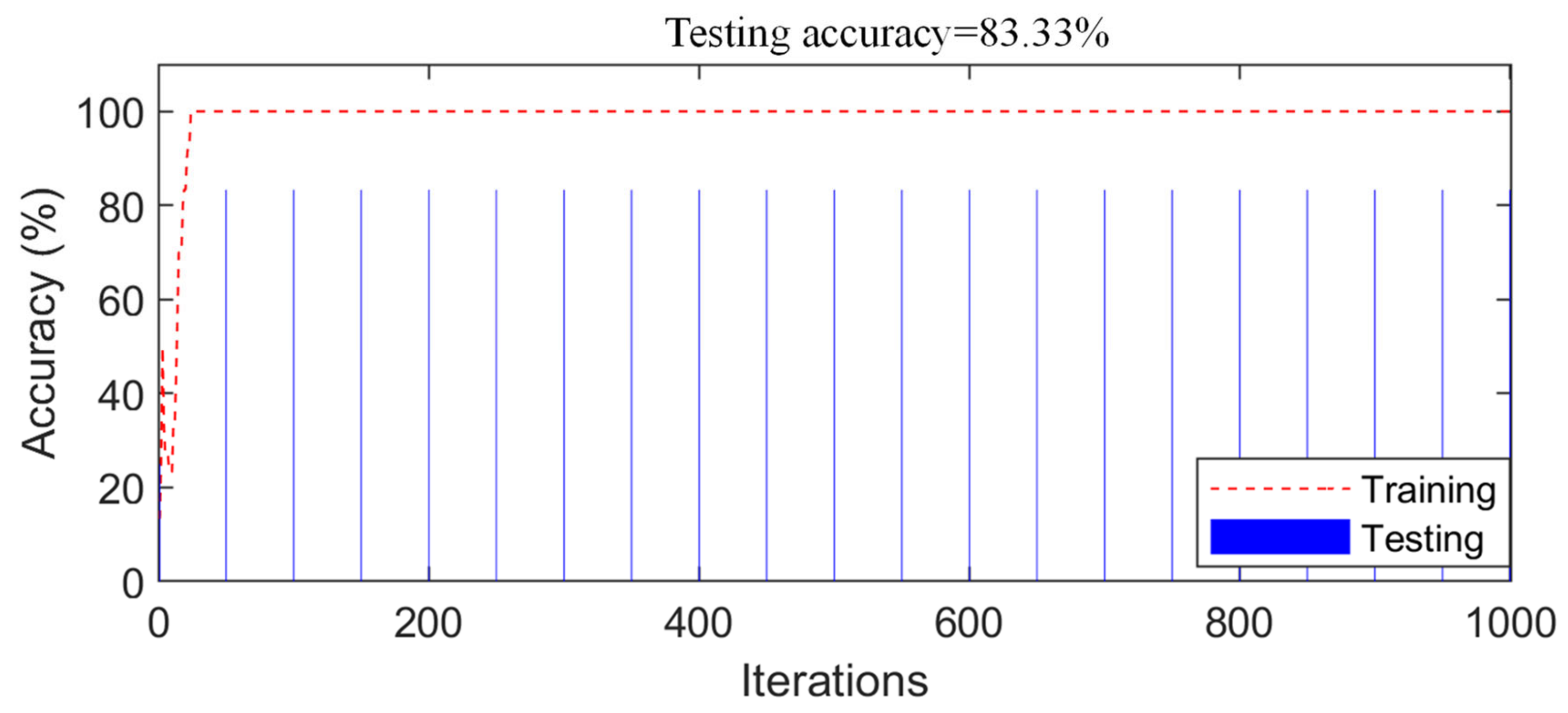
3.2. Detection Results of the Experimental Model
4. Conclusions
Supplementary Materials
Author Contributions
Funding
Institutional Review Board Statement
Informed Consent Statement
Data Availability Statement
Conflicts of Interest
Appendix A


References
- Yan, Y.J.; Cheng, L.; Wu, Z.Y.; Yam, L.H. Development in vibration-based structural damage detection technique. Mech. Syst. Signal Process. 2007, 21, 2198–2211. [Google Scholar] [CrossRef]
- An, Y.; Chatzi, E.; Sim, S.-H.; Laflamme, S.; Blachowski, B.; Ou, J. Recent progress and future trends on damage identification methods for bridge structures. Struct. Control Health Monit. 2019, 26, e2416. [Google Scholar] [CrossRef]
- Pandey, A.K.; Biswas, M.; Samman, M.M. Damage detection from changes in curvature mode shapes. J. Sound Vib. 1991, 145, 321–332. [Google Scholar] [CrossRef]
- Sung, S.H.; Koo, K.Y.; Jung, H.J. Modal flexibility-based damage detection of cantilever beam-type structures using baseline modification. J. Sound Vib. 2014, 333, 4123–4138. [Google Scholar] [CrossRef]
- Lu, Q.; Ren, G.; Zhao, Y. Multiple Damage Location with Flexibility Curvature and Relative Frequency Change for Beam Structures. J. Sound Vib. 2002, 253, 1101–1114. [Google Scholar] [CrossRef]
- Teng, S.; Chen, G.; Liu, G.; Lv, J.; Cui, F. Modal Strain Energy-Based Structural Damage Detection Using Convolutional Neural Networks. Appl. Sci. 2019, 9, 3376. [Google Scholar] [CrossRef]
- Cha, Y.; Buyukozturk, O. Structural Damage Detection Using Modal Strain Energy and Hybrid Multiobjective Optimization. Comput. Aided Civ. Infrastruct. Eng. 2015, 30, 347–358. [Google Scholar] [CrossRef]
- Ni, F.; Zhang, J.; Noori, M.N. Deep learning for data anomaly detection and data compression of a long-span suspension bridge. Comput. Aided Civ. Infrastruct. Eng. 2020, 35, 685–700. [Google Scholar] [CrossRef]
- Khuc, T.; Catbas, N. Completely contactless structural health monitoring of real-life structures using cameras and computer vision. Struct. Control Health Monit. 2017, 24, e1852. [Google Scholar] [CrossRef]
- Feng, G.; Yong, L. A Kalman-filter based time-domain analysis for structural damage diagnosis with noisy signals. J. Sound Vib. 2006, 297, 916–930. [Google Scholar]
- Ghiasi, R.; Torkzadeh, P.; Noori, M. A machine-learning approach for structural damage detection using least square support vector machine based on a new combinational kernel function. Struct. Health Monit. 2016, 15, 302–316. [Google Scholar] [CrossRef]
- Yam, L.H.; Yan, Y.J.; Jiang, J.S. Vibration-based damage detection for composite structures using wavelet transform and neural network identification. Compos. Struct. 2003, 60, 403–412. [Google Scholar] [CrossRef]
- Mehrjoo, M.; Khaji, N.; Moharrami, H.; Bahreininejad, A. Damage detection of truss bridge joints using Artificial Neural Networks. Expert Syst. Appl. 2008, 35, 1122–1131. [Google Scholar] [CrossRef]
- Gonzalez, M.P.; Zapico, J.L. Seismic damage identification in buildings using neural networks and modal data. Comput. Struct. 2008, 86, 416–426. [Google Scholar] [CrossRef]
- Chun, P.J.; Yamashita, H.; Furukawa, S. Bridge Damage Severity Quantification Using Multipoint Acceleration Measurement and Artificial Neural Networks. Shock Vib. 2015, 2015, 789384. [Google Scholar] [CrossRef]
- Lautour, O.; Omenzetter, P. Damage classification and estimation in experimental structures using time series analysis and pattern recognition. Mech. Syst. Signal Process. 2010, 24, 1556–1569. [Google Scholar] [CrossRef]
- Katunin, A.; Araújo dos Santos, J.V.; Lopes, H. Damage identification by wavelet analysis of modal rotation differences. Structures 2021, 30, 1–10. [Google Scholar] [CrossRef]
- Dackermann, U.; Li, J.; Samali, B. Dynamic-Based Damage Identification Using Neural Network Ensembles and Damage Index Method. Adv. Struct. Eng. 2010, 13, 1001–1016. [Google Scholar] [CrossRef]
- Zhong, K.; Teng, S.; Liu, G.; Chen, G.; Cui, F. Structural Damage Features Extracted by Convolutional Neural Networks from Mode Shapes. Appl. Sci. 2020, 10, 4247. [Google Scholar] [CrossRef]
- Lin, Y.Z.; Nie, Z.H.; Ma, H.W. Structural Damage Detection with Automatic Feature extraction through Deep Learning. Comput. Aided Civ. Infrastruct. Eng. 2017, 32, 1025–1046. [Google Scholar] [CrossRef]
- Teng, S.; Liu, Z.; Chen, G.; Cheng, L. Concrete Crack Detection Based on Well-Known Feature Extractor Model and the YOLO_v2 Network. Appl. Sci. 2021, 11, 813. [Google Scholar] [CrossRef]
- Yi, M.W.; Samali, B. Shake table testing of a base isolated model. Eng. Struct. 2002, 24, 1203–1215. [Google Scholar]
- Yu, Y.; Wang, C.; Gu, X.; Li, J. A novel deep learning-based method for damage identification of smart building structures. Struct. Health Monit. 2019, 18, 143–163. [Google Scholar] [CrossRef]
- Abdeljaber, O.; Sassi, S.; Avci, O.; Kiranyaz, S.; Ibrahim, A.A.; Gabbouj, M. Fault Detection and Severity Identification of Ball Bearings by Online Condition Monitoring. IEEE Trans. Ind. Electron. 2019, 66, 8136–8147. [Google Scholar] [CrossRef]
- Kiranyaz, S.; Gastli, A.; Ben-Brahim, L.; Alemadi, N.; Gabbouj, M. Real-Time Fault Detection and Identification for MMC using 1D Convolutional Neural Networks. IEEE Trans. Ind. Electron. 2018, 66, 8760–8771. [Google Scholar] [CrossRef]
- Abdeljaber, O.; Avci, O.; Kiranyaz, S.; Gabbouj, M.; Inman, D.J. Real-time vibration-based structural damage detection using one-dimensional convolutional neural networks. J. Sound Vib. 2017, 388, 154–170. [Google Scholar] [CrossRef]
- Avci, O.; Abdeljaber, O.; Kiranyaz, S.; Hussein, M.; Inman, D.J. Wireless and real-time structural damage detection: A novel decentralized method for wireless sensor networks. J. Sound Vib. 2018, 424, 158–172. [Google Scholar] [CrossRef]
- Zhang, Y.; Miyamori, Y.; Mikami, S.; Saito, T. Vibration-based structural state identification by a 1-dimensional convolutional neural network. Comput. Aided Civ. Infrastruct. Eng. 2019, 34, 822–839. [Google Scholar] [CrossRef]
- Nemec, S.F.; Donat, M.A.; Mehrain, S.; Friedrich, K.; Krestan, C.; Matula, C.; Imhof, H.; Czerny, C. CT-MR image data fusion for computer assisted navigated neurosurgery of temporal bone tumors. Eur. J. Radiol. 2007, 62, 192–198. [Google Scholar] [CrossRef] [PubMed]
- Ashraf, S.; Brabyn, L.; Hicks, B.J. Image data fusion for the remote sensing of freshwater environments. Appl. Geogr. 2011, 32, 619–628. [Google Scholar] [CrossRef]
- Tang, Z.; Chen, Z.; Bao, Y.; Li, H. Convolutional neural network-based data anomaly detection method using multiple information for structural health monitoring. Struct. Control Health Monit. 2019, 26, e2296. [Google Scholar] [CrossRef]
- Ernesto, G.; Maura, I. A multi-stage data-fusion procedure for damage detection of linear systems based on modal strain energy. J. Civil Struct. Health Monit. 2014, 4, 107–118. [Google Scholar]
- Teng, S.; Chen, G.; Gong, P.; Liu, G.; Cui, F. Structural damage detection using convolutional neural networks combining strain energy and dynamic response. Meccanica 2019, 55, 945–959. [Google Scholar] [CrossRef]
- Huo, Z.; Zhang, Y.; Shu, L. Bearing Fault Diagnosis using Multi-sensor Fusion based on weighted D-S Evidence Theory. In Proceedings of the 2018 18th International Conference on Mechatronics-Mechatronika (ME), Brno, Czech Republic, 5–7 December 2018; pp. 1–6. [Google Scholar]
- Li, J.; Zhu, X.; Law, S.S. A two-step drive-by bridge damage detection using Dual Kalman Filter. Int. J. Struct. Stab. Dyn. 2020, 20, 2042006. [Google Scholar] [CrossRef]
- Ying, L.; Feng, C.; Zhou, H. An algorithm based on two-step Kalman filter for intelligent structural damage detection. Struct. Control Health Monit. 2015, 22, 694–706. [Google Scholar]
- Xing, S.T.; Marvin, W. Application of substructural damage identification using adaptive Kalman filter. J. Civ. Struct. Health Monit. 2013, 4, 27–42. [Google Scholar] [CrossRef]
- Sen, S.; Bhattacharya, B. Online structural damage identification technique using constrained dual extended Kalman filter. Struct. Control Health Monit. 2017, 24, e1961. [Google Scholar] [CrossRef]
- Lai, Z.; Lei, Y.; Zhu, S. Moving-window extended Kalman filter for structural damage detection with unknown process and measurement noises. Measurement 2016, 88, 428–440. [Google Scholar] [CrossRef]
- Al-Hussein, A.; Haldar, A. Novel Unscented Kalman Filter for Health Assessment of Structural Systems with Unknown Input. J. Eng. Mech. 2015, 141, 04015012. [Google Scholar] [CrossRef]
- Huo, Z.; Miguel, M.G.; Zhang, Y. Entropy Measures in Machine Fault Diagnosis: Insights and Applications. IEEE Trans. Instrum. Meas. 2020, 69, 2607–2620. [Google Scholar] [CrossRef]
- Nie, Z.; Ngo, T.; Ma, H. Reconstructed Phase Space-Based Damage Detection Using a Single Sensor for Beam-Like Structure Subjected to a Moving Mass. Shock Vib. 2017, 2017, 5687837. [Google Scholar] [CrossRef]
- Scherer, D.; Müller, A.; Behnke, S. Evaluation of Pooling Operations in Convolutional Architectures for Object Recognition. In Proceedings of the International Conference on Artificial Neural Networks, Thessaloniki, Greece, 15–18 September 2010. [Google Scholar]
- Huang, J.; Li, D.; Zhang, C. Improved Kalman filter damage detection approach based on lp regularization. Struct. Control Health Monit. 2019, 26, e2424. [Google Scholar] [CrossRef]


| Layer | Type | Kernel Num. | Kernel Size | Stride | Activation |
|---|---|---|---|---|---|
| 1 | Input | None | None | None | None |
| 2 | Convolution (C1) | 128 | 3 × 1 | 1 | Leaky ReLU |
| 3 | Max pooling (P) | None | 2 × 1 | 1 | None |
| 4 | Convolution (C2) | 256 | 2 × 1 | 1 | Leaky ReLU |
| 5 | FC | None | None | None | None |
| 6 | Softmax | None | None | None | None |
| 7 | Classification | None | None | None | None |
| Sample | NNP1 | NNP2 | NNP3 | NNP4 | NNP5 | NNP6 | NNP7 |
|---|---|---|---|---|---|---|---|
| 1 | 1 | 1 | 5 | 1 | 8 | 5 | 2 |
| 2 | 6 | 4 | 5 | 1 | 9 | 6 | 6 |
| 3 | 8 | 6 | 6 | 5 | 10 | 9 | 8 |
| 4 | 9 | 7 | 8 | 5 | 11 | 11 | 11 |
| 5 | 9 | 16 | 9 | 10 | 11 | 11 | 13 |
| 6 | 13 | 18 | 10 | 13 | 15 | 14 | 17 |
| 7 | 13 | 18 | 10 | 15 | 18 | 15 | 19 |
| 8 | 14 | 19 | 14 | 20 | 19 | 17 | 26 |
| 9 | 14 | 19 | 19 | 21 | 20 | 18 | 27 |
| 10 | 17 | 22 | 20 | 21 | 23 | 20 | 27 |
| 11 | 21 | 23 | 20 | 22 | 29 | 23 | 28 |
| 12 | 21 | 25 | 20 | 23 | 32 | 25 | 31 |
| 13 | 30 | 25 | 22 | 24 | 32 | 25 | 31 |
| 14 | 32 | 26 | 22 | 31 | 34 | 27 | 33 |
| 15 | 32 | 31 | 36 | 31 | 34 | 28 | 36 |
| 16 | 34 | 35 | 39 | 34 | 35 | 31 | 36 |
| 17 | 37 | 36 | 43 | 34 | 36 | 32 | 36 |
| 18 | 38 | 39 | 45 | 36 | 37 | 37 | 37 |
| 19 | 39 | 40 | 52 | 42 | 37 | 40 | 38 |
| 20 | 41 | 45 | 54 | 43 | 39 | 49 | 38 |
| 21 | 42 | 46 | 55 | 44 | 41 | 49 | 43 |
| 22 | 47 | 49 | 56 | 48 | 42 | 50 | 45 |
| 23 | 48 | 51 | 58 | 53 | 43 | 52 | 49 |
| 24 | 49 | 54 | 59 | 54 | 45 | 54 | 49 |
| 25 | 57 | 55 | 55 | 46 | 54 | 50 | |
| 26 | 55 | 48 | 57 | 52 | |||
| 27 | 58 | 53 |
| Accuracy | Decision-Level Fusion | Improvement | |
|---|---|---|---|
| NNP1 | 89.41% | 100% | 10.59% |
| NNP2 | 88.98% | 11.02% | |
| NNP3 | 89.83% | 10.17% | |
| NNP4 | 89.41% | 10.59% | |
| NNP5 | 88.56% | 11.44% | |
| NNP6 | 88.98% | 11.02% | |
| NNP7 | 88.56% | 11.44% | |
| Average | 89.10% | 10.90% |
| Sample | NNP1 | NNP2 | NNP3 | NNP4 | NNP5 | NNP6 | NNP7 |
|---|---|---|---|---|---|---|---|
| 1 | 6 | 1 | 4 | 1 | 4 | 1 | 1 |
| 2 | 5 | 4 | 3 | 3 | |||
| 3 | 1 | 5 | 5 | ||||
| 4 | 2 | 6 | 5 | ||||
| 5 | 5 | 5 | |||||
| 6 | 1 | ||||||
| 7 | 1 |
| Accuracy | Decision-Level Fusion | Improved | |
|---|---|---|---|
| NNP1 | 91.67% | 100% | 8.33% |
| NNP2 | 95.83% | 4.17% | |
| NNP3 | 95.83% | 4.17% | |
| NNP4 | 70.83% | 29.17% | |
| NNP5 | 95.83% | 4.17% | |
| NNP6 | 83.33% | 16.67% | |
| NNP7 | 79.17% | 20.83% | |
| Average | 87.50% | 12.50% |
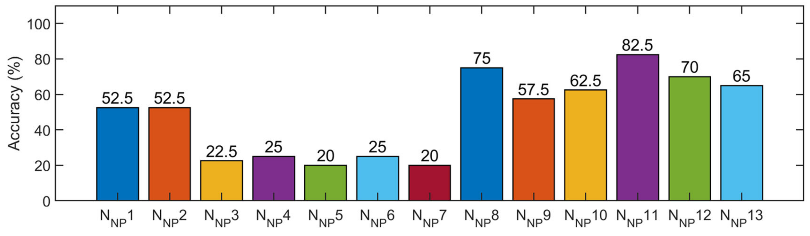
| Accuracy | Decision-Level Fusion | Improvement | |
|---|---|---|---|
| NNP1 | 52.50% | 85% | 47.50% |
| NNP2 | 52.50% | 47.50% | |
| NNP3 | 22.50% | 77.50% | |
| NNP4 | 25.00% | 75.00% | |
| NNP5 | 20.00% | 80.00% | |
| NNP6 | 25.00% | 75.00% | |
| NNP7 | 20.00% | 80.00% | |
| NNP8 | 75.00% | 25.00% | |
| NNP9 | 57.50% | 42.50% | |
| NNP10 | 62.50% | 37.50% | |
| NNP11 | 82.50% | 17.50% | |
| NNP12 | 70.00% | 30.00% | |
| NNP13 | 65.00% | 35.00% | |
| Average | 48.46% | 51.54% |
| Numerical Model (Bridge Model) | Experimental Model (Bridge Model) | Experimental Model (Steel Frame) | |
|---|---|---|---|
| Data-level fusion | 89.83% | 83.33% | 55.00% |
| Decision-level fusion | 100.00% | 100.00% | 85.00% |
| Improvement | 10% | 16% | 30% |
| Numerical Model (Bridge Model) | Experimental Model (Bridge Model) | Experimental Model (Steel Frame) | |
|---|---|---|---|
| Decision-level fusion | 100.00% | 100.00% | 85.00% |
| D–S evidence fusion | 98.31% | 100.00% | 10.00% |
| Improvement | 1.69% | 0% | 75% |
| Numerical Model (Bridge Model) | Experimental Model (Bridge Model) | Experimental Model (Steel Frame) | |
|---|---|---|---|
| Decision-level fusion | 721 s | 350 s | 1300 s |
| Data-level fusion | 488 s | 240 s | 510 s |
| D–S evidence fusion | 1073 s | 369 s | 1362 s |
Publisher’s Note: MDPI stays neutral with regard to jurisdictional claims in published maps and institutional affiliations. |
© 2021 by the authors. Licensee MDPI, Basel, Switzerland. This article is an open access article distributed under the terms and conditions of the Creative Commons Attribution (CC BY) license (https://creativecommons.org/licenses/by/4.0/).
Share and Cite
Teng, S.; Chen, G.; Liu, Z.; Cheng, L.; Sun, X. Multi-Sensor and Decision-Level Fusion-Based Structural Damage Detection Using a One-Dimensional Convolutional Neural Network. Sensors 2021, 21, 3950. https://doi.org/10.3390/s21123950
Teng S, Chen G, Liu Z, Cheng L, Sun X. Multi-Sensor and Decision-Level Fusion-Based Structural Damage Detection Using a One-Dimensional Convolutional Neural Network. Sensors. 2021; 21(12):3950. https://doi.org/10.3390/s21123950
Chicago/Turabian StyleTeng, Shuai, Gongfa Chen, Zongchao Liu, Li Cheng, and Xiaoli Sun. 2021. "Multi-Sensor and Decision-Level Fusion-Based Structural Damage Detection Using a One-Dimensional Convolutional Neural Network" Sensors 21, no. 12: 3950. https://doi.org/10.3390/s21123950
APA StyleTeng, S., Chen, G., Liu, Z., Cheng, L., & Sun, X. (2021). Multi-Sensor and Decision-Level Fusion-Based Structural Damage Detection Using a One-Dimensional Convolutional Neural Network. Sensors, 21(12), 3950. https://doi.org/10.3390/s21123950