Unified Chassis Control of Electric Vehicles Considering Wheel Vertical Vibrations

Abstract

In the process of vehicle chassis electrification, different active actuators and systems have been developed and commercialized for improved vehicle dynamic performances. For a vehicle system with actuation redundancy, the integration of individual chassis control systems can provide additional benefits compared to a single ABS/ESC system. This paper describes a Unified Chassis Control (UCC) strategy for enhancing vehicle stability and ride comfort by the coordination of four In-Wheel Drive (IWD), 4-Wheel Independent Steering (4WIS), and Active Suspension Systems (ASS). Desired chassis motion is determined by generalized forces/moment calculated through a high-level sliding mode controller. Based on tire force constraints subject to allocated normal forces, the generalized forces/moment are distributed to the slip and slip angle of each tire by a fixed-point control allocation algorithm. Regarding the uneven road, H∞ robust controllers are proposed based on a modified quarter-car model. Evaluation of the overall system was accomplished by simulation testing with a full-vehicle CarSim model under different scenarios. The conclusion shows that the vertical vibration of the four wheels plays a detrimental role in vehicle stability, and the proposed method can effectively realize the tire force distribution to control the vehicle body attitude and driving stability even in high-demanding scenarios.

1. Introduction

With the growing concern about pollution, energy shortage, and also fast development of electric propulsion technologies, modern vehicles are increasingly electrified. From the driver’s point of view, an adequate response in critical driving conditions is still a challenging task for non-professional drivers. Therefore, electric or electromechanical systems, featuring energy regeneration capability and fast response, are readily developed and applicated to improve the vehicle dynamics, from the aspects of comfort, stability, safety, maneuverability, and driver’s feeling, especially in adverse driving situations.

In order to enhance the driving stability and the overall dynamic performance, a vehicle may be equipped with multi-actuators, which can be classified into three categories as active torque distribution [1], active steering [2], and active suspension control [3]. Among all possible actuators, ABS-based differential braking has received the most attention since it can be executed on almost all vehicles regardless of powertrain configuration, known as the traditional ESC system. In 2003, the active front steering technology was developed and recognized as a supplemental approach to generate desired yaw moment without braking, ensuring enhanced vehicle stability even in high-speed conditions. However, the differential braking systems reduce the driving speed, which may conflict with the driver’s intention during acceleration scenarios. Concerning this defect, active torque distribution was implemented by two actuation methods: torque vectoring [4] and individual motors. The corresponding vehicle stability control method was called direct yaw control.

In most vehicle control approaches, different control logic based on various actuators are always separately synthesized and locally tuned without considering the interaction among them, which may lead to sub-optimal or conflicting control efforts. Nowadays, extensive research has been carried out on the coordination of active steering and independent torque control. Furthermore, the integration with active suspension systems provides a new research field under the name of global chassis control [5,6,7] or UCC (Unified Chassis Control) [8,9,10]. In general, most integrated control algorithms were developed using two different approaches concerning the actuators hierarchy: (1) In the first method, a supervisor with a higher command hierarchy was used to monitor vehicle states and coordinate different sub-controllers. As illustrated, sometimes the active steering was only considered if the differential braking system exceeded its limits or before the ESC was activated [11]. In [12], the coordination of active front steering and ESC was investigated using a rule-based method according to the different value ranges of lateral acceleration. (2) The second UCC category treated the overall control structure as two levels. In the upper-level, desired yaw moment was computed, then in the lower-level, the moment was distributed into tire forces [8,13].

From a control point of view, a variety of problems arise from the UCC system synthesis, such as multiple input–multiple output control design, system robustness, and non-linearity. Many researchers have tried to solve these challenges from the standpoints of reference track following and control optimization. Fuzzy logic was applied for an intermediate layer of a UCC method [14]. The sliding mode control technique, which possesses good robustness, was used to cope with system uncertainties [7,15]. In [11,16], control objectives were achieved in a linear parameter varying robust framework by providing a solution to the linear matrix inequality problem. The H∞-based observer is also designed for fault estimation and fault-tolerant control [17,18]. Model prediction control becomes a hotspot due to significant development on online computational devices [19,20,21]. Another challenge stemmed from how to achieve the constrained optimal allocation problems in systems with redundancy. In [9], the desired yaw moment distribution was algebraically solved by Karush–Kuhn–Tucker Conditions. Combined with the desired target following, energy minimization, and tire force saturation, the Holistic Cornering Control architecture was introduced [22,23]. Under this framework, the gain optimization was designed based on linear matrix inequality and genetic algorithm techniques. In [24], the redundant actuator allocation problem was investigated with pseudo-inverse and accelerated fix-point iterative algorithms. Since the tire normal load restraints the boundary of longitudinal and lateral force, the vertical force control indirectly influences the vehicle dynamics in the motion plane. The research in [25] has shown the possible benefits to be attained by modulating normal force through active suspension control during cornering maneuvers. Regarding the multiple targets of vehicle yaw performance and attitude, the integration control method involving suspensions and braking actuators was investigated in [26,27]. However, the integrated suspension control does not consider the tire contact stability.

Different from traditional vehicle chassis structures, the layout with four in-wheel motors is especially suitable for high-performance and off-road vehicles. However, this layout inevitably introduces a larger unsprung mass. With the development of in-wheel motor technology, it becomes a common judgment that the introduced unsprung mass aggravates the wheel vibration and vehicle ride comfort [28]. Especially when the vehicle is running over an uneven road, one or more of the wheels might jump, and the tires will lose adhesion stochastically, which leads to the unbalance of driving/braking torques among four wheels and even makes the vehicle encounter instability situations. This effect occurs not only for in-wheel drive electric vehicles but also for common vehicles. Till now, little research can be found in this area. Vos et al. [29] verified that the vertical accelerations caused by bad roads could increase the roll and pitch movement ranges. Zhang et al. [30] proposed the inference that the unsprung mass plays a different role in the rollover motion between a flat road and an uneven road, and verified it with typical situations. Tan et al. [31] investigated the negative effect of wheel motor vibration on vehicle anti-rollover performance. In addition, the tire contact stability has been given little attention in existing UCC designs.

The purpose of this work is to present a unified control framework with a particular focus on wheel vertical vibrations for enhanced tire contact stability. More specifically, we treat the multi-objective active suspension design problem as a robust tracking problem to achieve desired body attitude and normal forces simultaneously. Besides, a reconfigurable control allocation (CA) method is used to deal with the problematic condition of tire contact force loss due to an uneven road or tire blow-out emergency. Evaluation of the overall system was accomplished by simulation testing with a full-vehicle CarSim model under different test scenarios.

The remaining sections of this paper are organized as follows: Section 2 briefly presents the overall system modeling. In Section 3, nonlinear controller design and reconfigurable CA approach are presented, and the synthesis of the normal force controller considering different targets is described, followed by Section 4, which examines the closed-loop vehicle dynamics performance under different test scenarios through simulation results. Section 5 provides some concluding remarks.

2. System Modeling

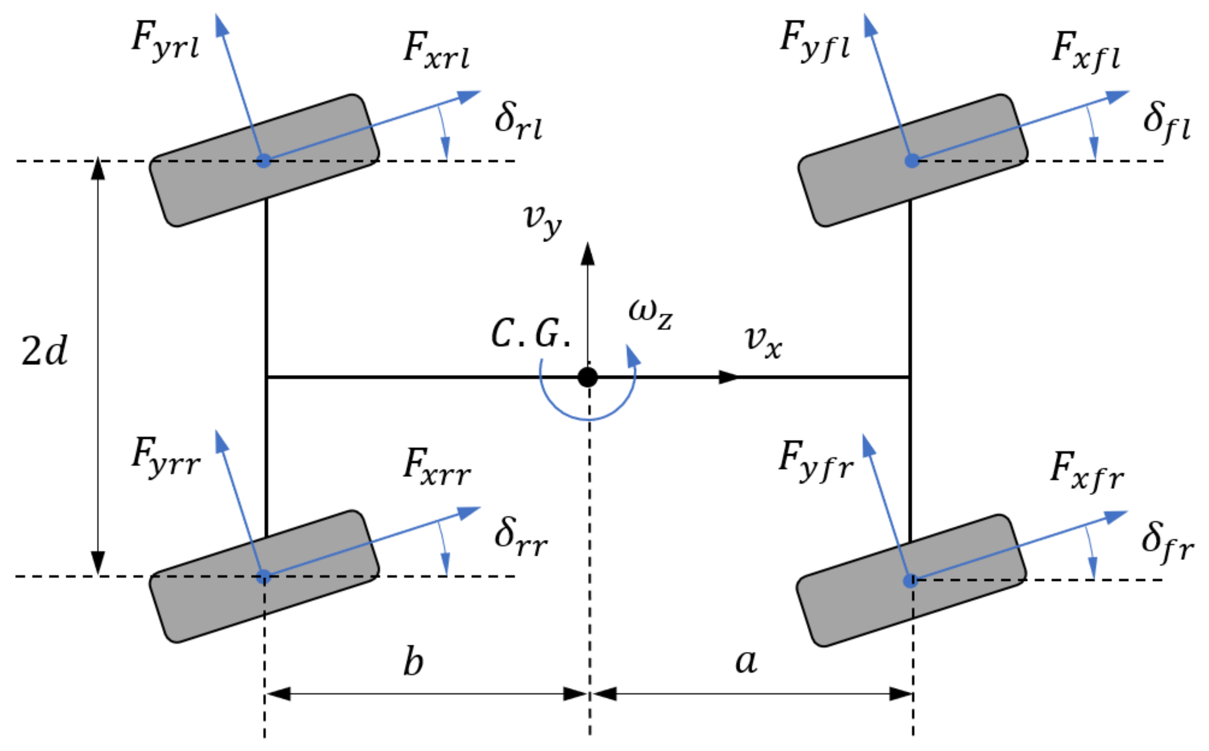
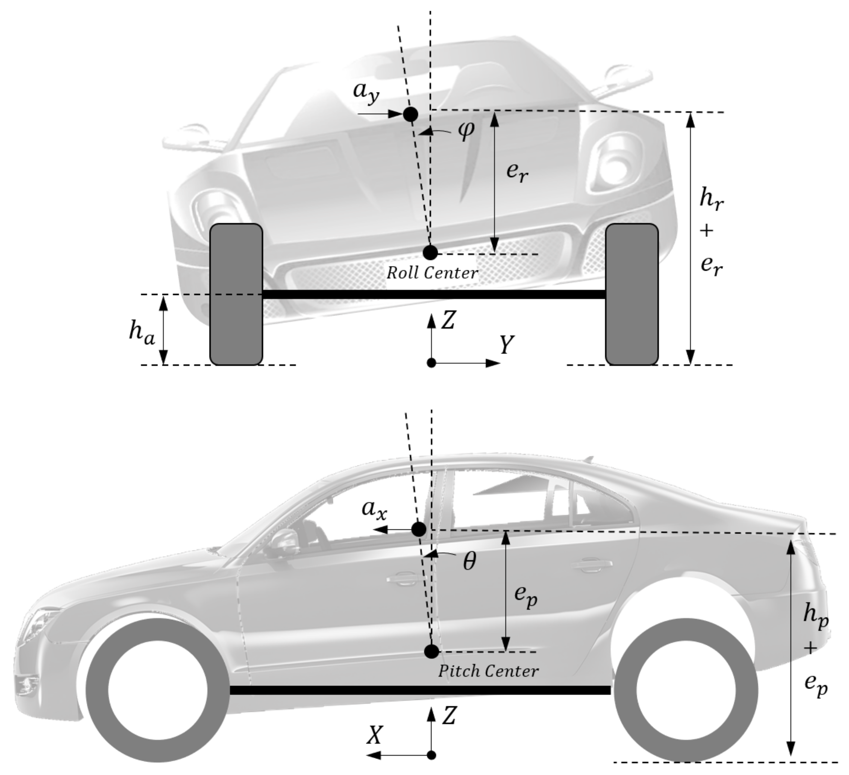
2.1. Nonlinear Vehicle Model

In this paper, both the chassis planar motion (longitudinal, lateral, and yaw) and the spatial motion (vertical, roll, and pitch) are considered. Thus, the vehicle body motion is treated as a rigid body with six degrees of freedom. Figure 1 shows the vehicle planar motion model. The dynamics equations of planar motions can be written as

$$\left\{\begin{array}{l}m\left({\dot{v}}_x-v_y{\omega }_z\right)+m_s{e}_r{\dot{\omega }}_z\phi =F_X-F_r\\ m\left({\dot{v}}_y+v_x{\omega }_z\right)-m_s{e}_r\ddot{\phi }=F_Y\\ I_{zz}{\dot{\omega }}_z=M_z\end{array}\right.,$$

(1)

with m as the vehicle mass (including the sprung mass m_s and unsprung mass m_u) and I_zz as the moment of inertia along Z-axis. The vehicle states are defined as the body motion velocity in three directions, namely (v_x v_y ω_z), with the vehicle coordinate system fixed at the vehicle Center of Gravity (CG). e_r denotes the distance of CG from the rolling center and φ is the rolling angle. The resultant forces exerted on the vehicle are defined as F_X, F_Y, and M_Z, with the following expressions

$$\left\{\begin{array}{l}{F}_X={\displaystyle \sum F_{Xi}}, i\in Q:=fl,fr,rl,rr\\ F_Y={\displaystyle \sum F_{Yi}}, i\in Q:=fl,fr,rl,rr\end{array}\right.,$$

(2)

$$M_Z=a\left(F_{Yfl}+F_{Yfr}\right)-b\left(F_{Yrl}+F_{Yrr}\right)+d\left(F_{Xfr}+F_{Xrr}-F_{Xfl}-F_{Xrl}\right)$$

(3)

F_r stands for the total longitudinal resistance. F_Xi and F_Yi are the tire forces under the vehicle coordinate system, whereas the longitudinal and lateral forces of a single tire under the tire coordinate system are expressed as F_xi and F_yi. Their relationship is described as follows.

$$\left[\begin{array}{c}{F}_{Xi}\\ F_{Yi}\end{array}\right]=\left[\begin{array}{cc}\cos {\delta }_i& -\sin {\delta }_i\\ \sin {\delta }_i& \cos {\delta }_i\end{array}\right]\left[\begin{array}{c}{F}_{xi}\\ F_{yi}\end{array}\right],i\in Q:=fl,fr,rl,rr$$

(4)

Figure 1. Vehicle planar motion model.

Figure 1. Vehicle planar motion model.

Considering the assumption that the vehicle has a four-wheel independent steering system, δ_i stands for the steering angle of a given wheel with the subscript representing the position which is controlled by every steering actuator. In Figure 2, the vehicle spatial motion models are illustrated. Concerning the unsprung mass dynamics, we treat the vehicle as a whole system under the influence of lateral and longitudinal accelerations.

Based on the reference direction in Figure 2, if we treat the sprung/unsprung mass as a whole system, the roll and pitch dynamic equations can be respectively expressed as

$$I_{xx}\ddot{\phi }=M_{\phi }+a_y{m}_s\left(h_r+e_r\right)+m_{s}g\phi e_r+a_y{m}_u{h}_a,$$

(5)

$$I_{yy}\ddot{\theta }+a_x{m}_s\left(h_p+e_p\right)+a_x{m}_u{h}_a=M_{\theta }+m_{s}g\theta e_p,$$

(6)

where, I_xx and I_yy are the principal moments of inertia of the vehicle body part along X and Y axis, respectively. (h_r + e_r) and (h_p + e_p) represent the heights of the rolling center and pitching center, respectively, with e_r as the distance between vehicle CG and rolling center and h_p as the distance between vehicle CG and pitching center. h_a represents the height of the unsprung mass center. The vehicle longitudinal/lateral accelerations can be calculated as,

$$a_x={\dot{v}}_x-v_y{\omega }_z, a_y={\dot{v}}_y+v_x{\omega }_z$$

These values are assumed to be available through a sensing system. Here, we ignore the mass of suspension links and assume that the unsprung mass CG is located in the wheel center. M_θ and M_φ denote the moments generated by the load transfer among vertical tire forces, and we describe this relationship in the form of

$$\left\{\begin{array}{l}{F}_{Zfl}={\overline{F}}_{Zfl}-\frac{M_{\theta }}{2(a+b)}+\frac{M_{\phi }}{4d},F_{Zfr}={\overline{F}}_{Zfr}-\frac{M_{\theta }}{2(a+b)}-\frac{M_{\phi }}{4d},\\ F_{Zrl}={\overline{F}}_{Zrl}+\frac{M_{\theta }}{2(a+b)}+\frac{M_{\phi }}{4d},F_{Zrr}={\overline{F}}_{Zrr}+\frac{M_{\theta }}{2(a+b)}-\frac{M_{\phi }}{4d},\end{array}\right.$$

(7)

where, F_Zi are static normal tire forces and F_Zi are desired tire normal forces, which can be achieved using four independent active suspension actuators.

2.2. Nonlinear Tire Model

We applied Pacejka’s Magic Formula tire model [32] to describe the nonlinear characteristics of tires, which is an empirical approach and can be effectively matched with experimental data. The longitudinal force, lateral force, and self-aligning moment of tire can be expressed by the following unified form with different parameter sets.

$$\left\{\begin{array}{l}y\left(x\right)=D\sin \left\{C\arctan \left[Bx-E\left(Bx-\arctan Bx\right)\right]\right\}\\ Y\left(X\right)=y(x)+S_v\\ x=X+S_h\end{array}\right.,$$

(8)

where Y represents the tire force that could be the longitudinal/lateral tire force or self-aligning moment. X denotes the model input, which corresponds to the tire slip or the slip angle. S_v and S_h correspond to the vertical and horizontal bias, respectively. Coefficients B, C, D, and E are the stiffness, shape, peak, and curvature factors, respectively. When considering the coupling of lateral and longitudinal force, we usually neglect the curvature factor for simplicity, and then the following relations hold approximately.

$$F_{xi}=\frac{{\sigma }_{xi}}{{\sigma }_i}{F}_{x0i},F_{yi}=\frac{{\sigma }_{yi}}{{\sigma }_i}{F}_{y0i}$$

(9)

F_x0i and F_y0i can be calculated by applying their corresponding magic formulas, with σ_xi as the longitudinal tire slip expressed below and σ_yi as the lateral tire slip.

$$\left\{\begin{array}{l}{\sigma }_{xi}=\frac{R_i{\omega }_i-v_{wxi}}{v_{wxi}}, \mathrm{during} \mathrm{braking}\\ {\sigma }_{xi}=\frac{R_i{\omega }_i-v_{wxi}}{R_i{\omega }_i}, \mathrm{during} \mathrm{acceleration}\end{array}\right.,$$

(10)

where, v_wxi expresses the velocity at tire center in the tire forward direction. According to the mentioned vehicle planar model, the slip angles of each wheel are

$$\left\{\begin{array}{l}{\alpha }_{fl}=-{\delta }_{fl}+\arctan \left(\frac{v_y+\dot{\psi }a}{v_x-\dot{\psi }d}\right)\approx -{\delta }_{fl}+\frac{v_y+\dot{\psi }a}{v_x-\dot{\psi }d}\\ {\alpha }_{fr}=-{\delta }_{fr}+\arctan \left(\frac{v_y+\dot{\psi }a}{v_x+\dot{\psi }d}\right)\approx -{\delta }_{fl}+\frac{v_y+\dot{\psi }a}{v_x+\dot{\psi }d}\\ {\alpha }_{fr}=-{\delta }_{rl}+\arctan \left(\frac{v_y-\dot{\psi }a}{v_x-\dot{\psi }d}\right)\approx -{\delta }_{fr}+\frac{v_y-\dot{\psi }a}{v_x-\dot{\psi }d}\\ {\alpha }_{rr}=-{\delta }_{rr}+\arctan \left(\frac{v_y-\dot{\psi }a}{v_x+\dot{\psi }d}\right)\approx -{\delta }_{rr}+\frac{v_y-\dot{\psi }a}{v_x+\dot{\psi }d}\end{array}\right.$$

(11)

Then, the lateral wheel slip is expressed as

$${\sigma }_{yi}=\frac{v_{wxi}}{R_i{\omega }_i}\tan {\alpha }_i,$$

(12)

and we have the resultant slip

$${\sigma }_i=\sqrt{{\sigma }_{xi}^2+{\sigma }_{yi}^2}$$

(13)

2.3. Driver Model

As to calculate the steering wheel input δ_sw, a standard preview-based controller in CarSim is used as a driver model, which minimized the vehicle deviations from the desired path for a given preview time. Further, the desired yaw motion is generated through a reference model, which describes the ideal vehicle responses based on vehicle speed and δ_sw, in the form of

$$\frac{{\omega }_{z,des}\left(s\right)}{{\delta }_{sw}\left(s\right)}=\frac{k_r{\overline{\omega }}_{z,des}}{\left(T_{1}s+1\right)\left(T_{2}s+1\right)},$$

(14)

$${\overline{\omega }}_{z,des}=\frac{v_x}{\left(a+b\right)+\frac{\left(b{C}_r-a{C}_f\right)m{v}_x^2}{2C_r{C}_f\left(a+b\right)}}$$

(15)

where k_r denotes the gain of the reference model. In this work, we set k_r = 0.05. T₁ and T₂ are tunning parameters. C_f and C_r represent the lateral stiffness of a single front/rear tire. Desired lateral velocity v_y,des is set to zero to avoid unnecessary tire lateral slip. Since the vehicle rollover can easily lead to fatal traffic accidents, it is necessary to prevent it through braking under rollover propensity quantitatively described by a Rollover Index (RI) that depends on the vehicle lateral acceleration and body roll angle [10]. When the index reaches the target warning value RI_th, brake control is adopted to prevent the vehicle from rolling over dangers. The RI is in the form of

$$\left\{\begin{array}{l}RI=C_1\left(\frac{\left|{\phi }_t\right|{\dot{\phi }}_{th}+{\phi }_{th}\left|{\dot{\phi }}_t\right|}{{\phi }_{th}{\dot{\phi }}_{th}}\right)+C_2\left(\frac{\left|a_y\right|}{a_{y,c}}\right)+\left(1-C_1-C_2\right)\frac{\left|{\phi }_t\right|}{\sqrt{{\phi }_t^2+{\dot{\phi }}_t^2}}, \mathrm{if} \phi \left(\dot{\phi }-k\phi \right)\ge 0\\ RI=0, \mathrm{if} \phi \left(\dot{\phi }-k\phi \right)<0\end{array}\right.$$

(16)

When the RI reaches the defined target value RI_th, we control the lateral acceleration by braking to reduce the RI down to RI_th, and the desired lateral acceleration is described as

$$\left|a_{y,des}\right|=\frac{a_{y,c}}{C_2}[R{I}_{des}-C_1\left(\frac{\left|{\phi }_t\right|{\dot{\phi }}_{th}+{\phi }_{th}\left|{\dot{\phi }}_t\right|}{{\phi }_{th}{\dot{\phi }}_{th}}\right)-\left(1-C_1-C_2\right)\frac{\left|{\phi }_t\right|}{\sqrt{{\phi }_t^2+{\dot{\phi }}_t^2}}]$$

(17)

Considering the relationship between vehicle lateral acceleration and driving speed

$$a_{y,des}={\dot{v}}_y+v_{x,des}{\omega }_z,$$

(18)

$$a_y={\dot{v}}_y+v_x{\omega }_z$$

(19)

It follows that

$$v_{x,des}=v_x+\frac{1}{{\omega }_z}\left(a_{y,des}-a_y\right)$$

(20)

Otherwise, we consider the desired longitudinal speed as a constant cruising value when the RI was controlled within a reasonable range. Then the desired vehicle speed becomes

$$v_{x,des}=v_{x,cons}$$

(21)

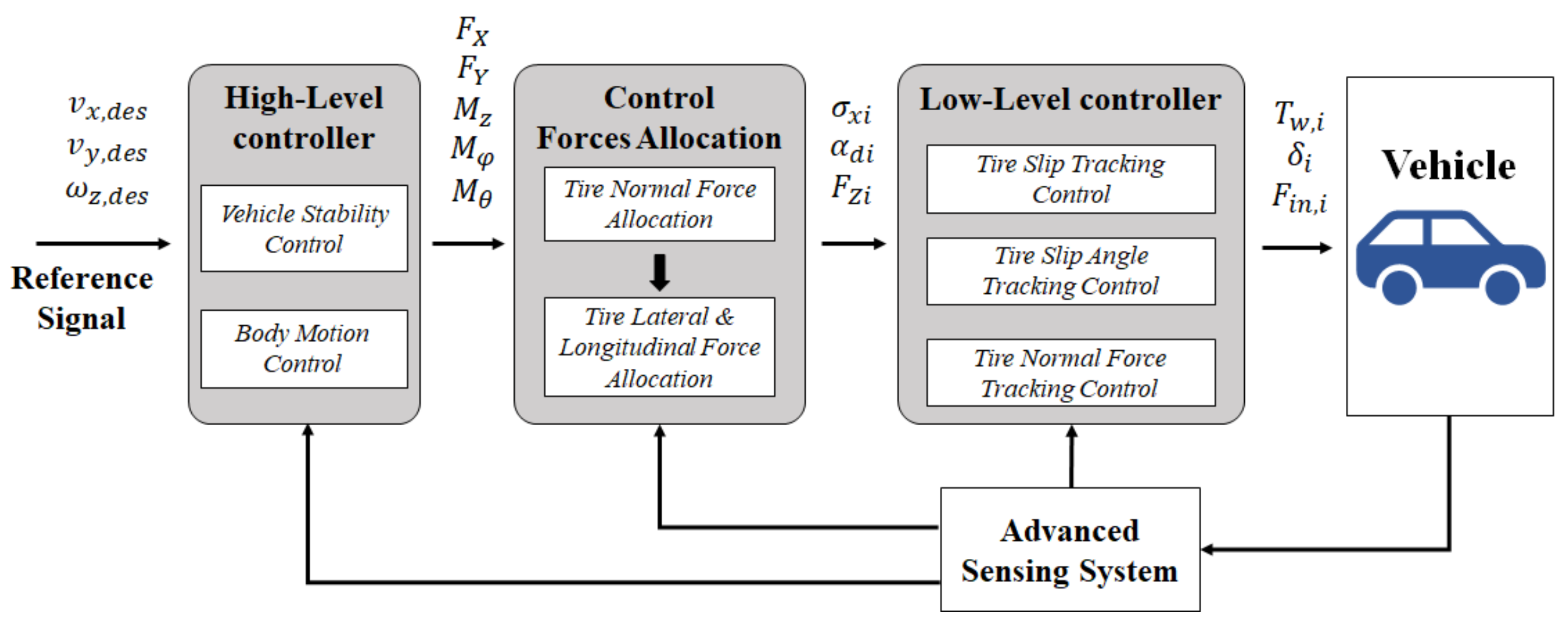
3. Design of the Control System

For a UCC design with all four wheels having independent torque, suspension, and steering-by-wire functions, the vehicle works as a redundantly actuated system. A hierarchical control structure shown in Figure 3 is presented to coordinate different control subsystems by the allocation of tire forces.

In this scheme, the high-level controller determines the resultant force/moment affected on the vehicle according to the control targets, including both the vehicle lateral stability and the spatial body motion (roll and pitch). Regarding the desired body motion dynamics, the target values of lateral and longitudinal transfer among the normal forces of every tire can be obtained. With the allocated normal forces through active suspension control, the CA algorithm distributes the resultant lateral and longitudinal forces to every wheel, which are finally realized through the closed-loop tracking control methods by considering the nonlinear tire model. In this work, we ignore the tire transient dynamics and assume that the desired tire longitudinal/lateral forces are well tracked through the variation of wheel steering angle δ_i and the driving/braking torque T_w,i. The steering angle of each wheel can be obtained through (11) with the desired value of wheel slip angle. According to the desired wheel longitudinal forces, T_w,i are calculated as,

$$T_{w,i}=J_{w,i}{\dot{\omega }}_{w,i}+F_{x,i}{r}_{w,i},$$

(22)

where J_w,i include the wheel-side inertia. r_w,i and ω_w,i are the radius and the angular speed of the wheels, respectively. The values of δ_i and T_w,i are treated as the inputs of the vehicle model in simulations. We also assume that all necessary quantitires in the control design can be practically measured or estimated.

3.1. High-Level Robust Controller Design

Parameter uncertainty is a common issue that requires robustness in control design. Compared with the actual vehicle model, common parameters with uncertainty include vehicle mass m, the inertia of moment I_xx, I_yy, I_zz, rolling center position e_r, pitching center position e_p, unmodeled dynamics such as suspension dynamics, and disturbance like wind gust and road roughness. Addressing the vehicle non-linearity and mentioned system uncertainties, a sliding mode controller is proposed for system robustness based on the simplified dynamics. If we define the system states as

$$x_i=[v_x,v_y,\dot{\psi },\dot{\phi },\dot{\theta }]$$

The vehicle system can be given in state-space form as

$$\left\{\begin{array}{l}{\dot{x}}_1=x_2{x}_3-\frac{1}{m}{F}_r-\frac{m_s}{m}{e}_r{\dot{x}}_3{x}_4+\frac{1}{m}{u}_1+{\Delta }_1\\ {\dot{x}}_2=-x_1{x}_3+\frac{m_s}{m}{e}_r{\dot{x}}_4+\frac{1}{m}{u}_2+{\Delta }_2\\ {\dot{x}}_3=\frac{1}{I_{zz}}{u}_3+{\Delta }_3\\ {\dot{x}}_4=\frac{a_y\left[m_s\left(h_r+e_r\right)+m_u{h}_a\right]}{I_{xx}}+\frac{m_{s}g{e}_r\phi }{I_{xx}}+\frac{1}{I_{xx}}{u}_4+{\Delta }_4\\ {\dot{x}}_5=-\frac{a_x\left[m_s\left(h_p+e_p\right)+m_u{h}_a\right]}{I_{yy}}+\frac{m_{s}g{e}_p\theta }{I_{yy}}+\frac{1}{I_{yy}}{u}_5+{\Delta }_5\end{array}\right.$$

(23)

where ∆_i stand for unmodeled dynamics. The control inputs are defined as

$$\left(u_1,u_2,u_3,u_4,u_5\right)=\left(F_X,F_Y,M_z,M_{\phi },M_{\theta }\right)$$

These equations can be treated as five single-input-single-output systems, then the control inputs u₁,…,u₅ become decoupled. Next, we select the velocity error as the sliding surface for state x₁, x₂, and x₃ for the path following purpose. Considering that the body roll and pitch motions should not be avoided completely for tire contact stability, we design dynamics sliding surfaces for the other two states.

$$\left\{\begin{array}{l}{S}_n=e_n=x_n-x_{n,des}, n=1,2,3\\ S_n=x_4+C_{\phi }\phi , n=4\\ S_n=x_5+C_{\theta }\theta , n=5\end{array}\right.$$

(24)

In this paper, we turn the coefficients as C_φ = C_θ = 1. For each channel, the Lyapunov function candidate is in the form of

$$V_n=\frac{1}{2}{S}_n^2$$

(25)

To achieve the attractive behavior of the sliding surface in a finite time period, it follows that

$${\dot{V}}_n=S_n{\dot{S}}_n\le -{\eta }_n\left|S_n\right|$$

(26)

where the value of η_n(>0) decides the speed of sliding surface convergence. The attractive equations can be given as

$${\dot{S}}_n=-K_{n}Sign\left(S_n\right)$$

(27)

Taking channel one as example, we have

$$x_2{x}_3-\frac{F_r}{m}-\frac{m_s}{m}{e}_r{\dot{x}}_3{x}_4+\frac{1}{m}{u}_1+{\Delta }_1-{\dot{x}}_{1,des}=-K_{1}Sign\left(S_1\right)$$

(28)

In practical use, some system parameters remain unknown to control design. Thus, the desired control efforts can only be expressed based on the nominal values, such as

$$u_1=\overline{m}[-x_2{x}_3+\frac{F_r}{\overline{m}}+\frac{{\overline{m}}_s}{\overline{m}}{\overline{e}}_r{\dot{x}}_3{x}_4+{\dot{x}}_{1,des}-{\overline{\Delta }}_1-K_{1}Sign\left(S_1\right)]$$

(29)

Substituting this value into (26), it follows that

$${\dot{V}}_1=S_1\left\{\left(1-\frac{\overline{m}}{m}\right)x_2{x}_3+\left(\frac{{\overline{m}}_s{\overline{e}}_r}{m}-\frac{m_s{e}_r}{m}\right){\dot{x}}_3{x}_4+\left(\frac{\overline{m}}{m}-1\right){\dot{x}}_{1,des}+\left({\Delta }_1-\frac{\overline{m}}{m}{\overline{\Delta }}_1\right)-\frac{\overline{m}}{m}{K}_{1}Sign\left(S_1\right)\right\}$$

(30)

Here, we select the nominal values as

$$\left\{\begin{array}{l}\overline{m}=\sqrt{m_{\min }{m}_{\max }}, {\beta }_m^{-1}\le \frac{\overline{m}}{m}\le {\beta }_m\\ {\overline{m}}_s=\sqrt{m_{s,\min }{m}_{s,\max }}, {\beta }_{ms}^{-1}\le \frac{{\overline{m}}_s}{m_s}\le {\beta }_{ms}\\ {\overline{e}}_r=\sqrt{e_{r,\min }{e}_{r,\max }}, {\beta }_{er}^{-1}\le \frac{{\overline{e}}_r}{e_r}\le {\beta }_{er}\end{array}\right.$$

(31)

where,

$${\beta }_m=\sqrt{\frac{m_{\max }}{m_{\min }}},{\beta }_{ms}=\sqrt{\frac{m_{s,\max }}{m_{s,\min }}},{\beta }_{er}=\sqrt{\frac{e_{r,\max }}{e_{r,\min }}}$$

Then all factors in (30) have corresponding upper bounds

$$\left\{\begin{array}{l}\left|1-\frac{\overline{m}}{m}\right|\le \max \left\{\left|1-{\beta }_m^{-1}\right|,\left|1-{\beta }_m\right|\right\}={\overline{\beta }}_{11}\\ \left|\frac{{\overline{m}}_s{\overline{e}}_r}{m}-\frac{m_s{e}_r}{m}\right|\le \max \left\{\left|1-{\beta }_{ms}^{-1}{\beta }_{er}^{-1}\right|,\left|1-{\beta }_{ms}{\beta }_{er}\right|\right\}{e}_{r,\max }={\overline{\beta }}_{12}\\ \left|{\Delta }_1-\frac{\overline{m}}{m}{\overline{\Delta }}_1\right|\le \max \left\{\left|{\Delta }_{1,\max }\right|,\left|{\Delta }_{1,\min }\right|\right\}+{\beta }_m\left|{\overline{\Delta }}_1\right|={\overline{\beta }}_{13}\end{array}\right.$$

(32)

Due to the assumption that all the vehicle states and their derivates are physically upper bounded, Equation (30) becomes

$${\dot{V}}_1\le \left[{\overline{\beta }}_{11}{\left|x_2{x}_3\right|}_m+{\overline{\beta }}_{12}{\left|{\dot{x}}_3{x}_4\right|}_m+{\overline{\beta }}_{11}{\left|{\dot{x}}_{1,des}\right|}_m+{\overline{\beta }}_{13}-{\beta }_m^{-1}{K}_1\right]\left|S_1\right|\le -{\eta }_1\left|S_1\right|$$

(33)

In order to achieve the convergence inequality, it is then sufficient to have

$$K_1\ge {\beta }_m\left({\overline{\beta }}_{11}{\left|x_2{x}_3\right|}_m+{\overline{\beta }}_{12}{\left|{\dot{x}}_3{x}_4\right|}_m+{\overline{\beta }}_{11}{\left|{\dot{x}}_{1,des}\right|}_m+{\overline{\beta }}_{13}+{\eta }_1\right)$$

(34)

To avoid the chattering effects caused by the switching function, it is replaced by a saturation function, which is a continuous approximation with the thickness of ϕ₁, and then the control law of channel 1 becomes

$$u_1=\overline{m}[-x_2{x}_3+\frac{1}{2\overline{m}}CA{x}_1^2+\frac{{\overline{m}}_s}{\overline{m}}{\overline{e}}_r{\dot{x}}_3{x}_4+{\dot{x}}_{1,des}-{\overline{\Delta }}_1-K_{1}Sat\left(\frac{S_1}{{\varphi }_1}\right)]$$

(35)

Through the same process, the control laws for other sliding surfaces are

$$u_2=\overline{m}\left[x_1{x}_3+\frac{{\overline{m}}_s}{\overline{m}}{\overline{e}}_r{\dot{x}}_4+{\dot{x}}_{2,des}-{\overline{\Delta }}_2-K_{2}Sat\left(\frac{S_2}{{\varphi }_2}\right)\right]$$

(36)

$$u_3={\overline{I}}_{zz}\left[{\dot{\omega }}_{z,des}-{\overline{\Delta }}_3-K_{3}Sat\left(\frac{S_3}{{\varphi }_3}\right)\right]$$

(37)

$$u_4=-a_y\left[{\overline{m}}_s\left({\overline{h}}_r+{\overline{e}}_r\right)+{\overline{m}}_u{h}_a\right]-{\overline{m}}_s{\overline{e}}_{s}g\phi +{\overline{I}}_{xx}\left[-C_{\phi }{x}_4-{\overline{\Delta }}_4-K_{4}Sat\left(\frac{S_4}{{\varphi }_4}\right)\right]$$

(38)

$$u_5=a_x\left[{\overline{m}}_s\left({\overline{h}}_p+{\overline{e}}_p\right)+{\overline{m}}_u{h}_a\right]-{\overline{m}}_s{\overline{e}}_{p}g\theta +{\overline{I}}_{yy}\left[-C_{\theta }{x}_5-{\overline{\Delta }}_5-K_{5}Sat\left(\frac{S_5}{{\varphi }_5}\right)\right]$$

(39)

For every channel, by choosing the K_n to be sufficiently large, the convergence inequalities can be guaranteed, and the sliding surfaces are designed to be attractive. In this paper, we choose K₁ = 0.02, K₂ = 0.2, K₃ = 0.01, K₄ = 0.1, and K₅ = 0.1. Through the appropriate CA method, the high-level control efforts u₁-u₅ are distributed into four wheels. However, we cannot always achieve these control efforts considering that the tire forces are generated through the contact behavior between tires and road and are physically bounded.

3.2. Control Allocation Algorithm

The hierarchical control algorithm with a redundant set of actuators frequently contains a high-level controller to generate virtual control efforts and a control allocation algorithm to coordinate the actuators to produce the desired control values together. If the control efforts require forces beyond the capabilities of the actuators due to saturation or physical limitations, the CA algorithm should be able to lower its performance and search for a control input vector that minimized the error. Additionally, redundant actuators can be utilized to provide fault tolerance for safety-critical conditions such as normal force losing. For real-time applications, the computational effort is also an essential property for choosing the CA algorithm. In this viewpoint, we applied a fixed-point CA method to solve the CA problem in constraint system control. Based on the nonlinear vehicle and tire models, the generalized force/moment can be expressed using a set of nonlinear functions of control variables

$$u_d=F\left(\lambda ,U\right),$$

(40)

where, $\lambda ={\left[F_{zi},{\mu }_i,{\delta }_i\right]}^T$ is a 12 × 1 vector configurating the CA problem and remains invariable during a CA computation step. ¦Ì_i is the friction coefficient between road and tires. $U={\left[{\alpha }_i,{\kappa }_i\right]}^T$ is a 8 × 1 control vector of slip angle and slip ratio of each tire. u_d denotes the desired generalized force, which can be rewritten using a first-order linearizing expression about an operating point,

$$\begin{array}{l}F\left(\lambda ,U\right)\approx F\left(\lambda ,U_{k-1}\right)+\frac{\partial F}{\partial U}\left(\lambda ,U_{k-1}\right)\cdot \left(U_k-U_{k-1}\right)\Rightarrow \\ F\left(\lambda ,U\right)-F\left(\lambda ,U_{k-1}\right)+\frac{\partial F}{\partial U}\left(\lambda ,U_{k-1}\right)\cdot U_{k-1}=\frac{\partial F}{\partial U}\left(\lambda ,U_{k-1}\right)\cdot U_k=B_F\cdot U_k\end{array}$$

(41)

where, B_F is a Jacobian matrix defined by the configurating vector and the control vector of the last step, which describes the sensitivity of the control vector to desired value vector u′_d, which is in the form of

$${u^{\prime }}_d=u_d-F\left(\lambda ,U_{k-1}\right)+\frac{\partial F}{\partial U}\left(\lambda ,U_{k-1}\right)\cdot U_{k-1}$$

(42)

Then, Equation (41) becomes

$${u^{\prime }}_d\approx B_F\cdot U_k$$

(43)

The CA algorithm minimized the following objective function, including the CA errors and control effort. The optimization criteria can be given as

$$\min J=\frac{1}{2}\left(1-\epsilon \right){\mathsf{\Gamma }}^T{W}_e\mathsf{\Gamma }+\frac{1}{2}\epsilon U^T{W}_{U}U$$

(44)

where Γ = (B_FU − u′_d) is the control error vector, and the variation of control value U∈[U_L, U_U] is restrained by actuator rate limits and achievable value ranges. The two bounds are decided by

$$\left\{\begin{array}{l}{U}_L=\max [U_{\min },U_{k-1}-\tau \cdot r_{\max }]\\ U_U=\min [U_{\max },U_{k-1}+\tau \cdot r_{\max }]\end{array}\right.$$

(45)

where, τ represents the sampling time and r_max is the maximum rates of variable values. This constraint helps to ensure the process stability. ε is a number to balance the weight between control efforts error and actuation cost, which is chosen as 0.5. Suppose that we want to minimize J:R⁸→R, a gradient descent algorithm has the iterative step

$$U_{i+1}=U_i-\eta \nabla J\left(U_i\right)$$

(46)

∇J(U) is the derivative of J at U. Substituting the derivative of J into this equation. It follows that

$$\left\{\begin{array}{l}{U}_{i+1}=sat\left[\left(1-\epsilon \right)\eta B_F^T{W}_e{u^{\prime }}_d-\left(\eta T-I\right)U_i\right]:=I\left(U_i\right)\\ T=\left(1-\epsilon \right)B_F^T{W}_e{B}_F+\epsilon W_U\end{array}\right.$$

(47)

where the step length parameter η is set to η = 1/‖T‖_F, with ‖·‖_T being the Frobenius norm of a matrix, which is more computationally efficient than induced norms. The saturation function sat can cut the elements of the control vector U_(i+1) at their limits. If J is convex and the operator I is convergent, then a point U_k is a fixed point of I if and only if ∇J(U_k) = 0, so if and only if U_k minimizes J, with the expression

$$U_k=I\left(U_k\right)$$

(48)

3.3. Tire Normal Forces Robust Tracking Control

Based on the mentioned tire models, the boundaries of friction ellipses are directly affected by the normal tire forces, which are the control vectors of the high-level strategy for inhibiting undesired vehicle motion. The tracking control based on the active suspension system is a challenging task because of the following reasons.

(1)

In practical use, the wheel motions are under the effect of road roughness, especially considering the high unsprung mass introduced by the electric propulsion system, such as the in-wheel motor. This kind of motion instability will cause the inaccuracy of tire load tracking.

(2)

Quarter car model is the classic model which was widely utilized in suspension analysis and control synthesis. However, the spatial kinematics and dynamics considering the suspension geometry are relatively complicated, leading to the inaccuracy and uncertainty of model parameters. Though some analytic model of suspension geometry is presented and realized in simulation [33], the complex computation makes them less efficient in real-car implements.

(3)

The active suspension control algorithm is always a trade-off between the vehicle ride comfort and tire-road adhesion stability, which is hard to be optimized simultaneously. Moreover, the tracking control requirement makes the problem more complex and increases the difficulty of controller design.

In this work, we used the traditional quarter car model and H-∞ robust control method to solve the modeling uncertainty and parameter variation problem. The model concept is illustrated through Figure 4, with M_b as the one-fourth sprung mass, M_w as the one-fourth unsprung mass, k_s as the equivalent suspension stiffness, b_s as the equivalent suspension damping, and k_t as the tire stiffness. The force from the vehicle body F_in is a known input. F_a is the active force returned by the active suspension controller.

Based on the traditional quarter car model, an extra equivalent body inertia force F_in is imposed upon the sprung mass to reflect the coupling effect between the quarter model and the full-vehicle model. The value of F_in is supposed to be the desired normal tire force. Due to suspension geometry and ride comfort requirements, the equivalent suspension stiffness and damping are actually not constant values, which is treated as system uncertainties. The body inertia force and road profile are the outside disturbances to the system. However, we can still use their nominal values to establish the model. The states of the controlled system are defined as $\left[x_1,x_2,x_3,x_4\right]=\left[x_w,{\dot{x}}_w,x_b,{\dot{x}}_b\right]$, and generalized system inputs are $\left[u_1,u_2,u_3\right]=\left[F_{in},x_g,F_a\right]$.

Then, the vertical dynamics of suspension can be given as

$$\left\{\begin{array}{l}{\dot{x}}_2=-\left(\frac{k_s+k_t}{M_w}\right)x_1-\frac{b_s}{M_w}{x}_2+\frac{k_s}{M_w}{x}_3+\frac{b_s}{M_w}{x}_4+\frac{k_t}{M_w}{u}_2-\frac{1}{M_w}{u}_3\\ {\dot{x}}_4=\frac{k_s}{M_b}{x}_1+\frac{b_s}{M_b}{x}_2-\frac{k_s}{M_b}{x}_3-\frac{b_s}{M_b}{x}_4-\frac{1}{M_b}{u}_1+\frac{1}{M_b}{u}_3\end{array}\right.$$

(49)

The system performance index is selected as

$$Y_{perf}=\left[{\ddot{x}}_b,e_n,F_a\right]$$

(50)

where the sprung mass acceleration is the index for ride comfort, and e_n = F_in − k_t(x_g − x_w) expresses the normal force control error, defined as the tire contact stability index. F_a stands for the active suspension actuator force. The system output includes the performance index as well as the signals to be measured for feedback control, which may contain the body (unsprung mass) acceleration (BA) and tire dynamic load (DL). We use the linear fractional transformation method to define an extended state-space model to deal with the parameter uncertainties. The closed-loop system diagram is described in Figure 5 [34].

The weighting functions of system performance index W_ba, W_tl, and control output and W_u, which define the target performance in the frequency domain, should be well tuned to acquire a stable and satisfactory controller. Here, we design and tune the weighting function according to the open-loop suspension performance, and the amplitude-frequency characteristics of BA and DL are compared with the inverse of the weighting function W_ba and W_tl in Figure 6. Furthermore, since the desired characteristic of BA and DL is hard to achieve simultaneously, we use different control structures to achieve the vehicle comfort target and tire stability target:

(1)

Controller 1: For the state of tire contact force cannot reflect the dynamic behavior of sprung mass, only the sprung mass acceleration was selected as the feedback signal of the comfort-orientated control scheme.

(2)

Controller 2: In the tire-stability-orientated control scheme, both the unsprung mass acceleration and tire contact force work as the feedback signals, with the former signal reflecting the desired tire normal force and the latter one providing the real normal force. The sensor reflects the DL could be tire-pressure based, for example.

In order to compare the performance of the closed-loop system of controller 1 and controller 2, the state-space system models are established in the MATLAB environment, where the corresponding H-∞ controllers are synthesized through coupled Riccati equations [35]. Further, a sinusoidal input was built to test the tracking performance of controller 2. Simulation results concerning body acceleration and tire dynamic load in the time domain are shown in Figure 7. Their root mean square values are listed in

Table 1. RMS values of body acceleration and tire dynamic load.

Suspension Performances	Passive Suspension (without Control)	Comfort-Orientated Control	Stability-Orientated Control
Body acceleration (m/s2)	0.6732	0.2795 (↓58%)	0.9067 (↑35%)
Tire dynamic load (N)	242.7421	377.5729 (↑56%)	204.7990 (↓16%)

for comparison. An A-class uneven road is simulated by filtered white noise according to ISO8608, with the vehicle speed chosen as 120 km/h.

Figure 6. The inverse of system performance index weighting functions: (a) vertical acceleration; (b) tire dynamic load.

Figure 6. The inverse of system performance index weighting functions: (a) vertical acceleration; (b) tire dynamic load.

The simulation results illustrate that, under the comfort-oriented control, the body acceleration magnitude illustrated by the blue line was decreased, compared with the value without active control expressed by the black line. On the contrary, the average tire DL was increased. Reversely, the stability-oriented control inhibited the normal tire force tracking error but enlarged the body acceleration magnitude unavoidably. Results in Figure 8 indicated that controller 2 achieved good tracking performance under sinusoidal input signal with the suppression of road roughness disturbance.

Although we only consider the tracking control of tire vertical forces, energy consumption of the active suspension system cannot be neglected. The tradeoff between vibration suppression and energy consumption should be considered in practical applications, which could be realized by adjusting the weighting funcion W_u.

4. Simulation Studies

In order to evaluate its overall performance, the UCC system with the application of the stability-oriented controller (controller 2) is implemented in a CarSim–Simulink co-simulation platform. The target vehicle is a B-class sports car. Its parameters are listed in

Table 2. Vehicle parameters in the simulation.

Symbol	Description	Values and Units
m	Vehicle mass	1140 kg
CD	Aerodynamic drag coefficient	0.34
a	Distance of front wheel axle from C.G.	1.165 m
b	Distance of rear wheel axle from C.G.	1.165 m
d	Half of the wheel base	0.7405 m
Izz	Yaw inertia	996 kg m2
ms	Vehicle sprung mass	1020 kg
ks	Suspension stiffness	33,972 N/m
bs	Suspension damping	2000 N s/m
kt	Tire stiffness	200,000 N/m

. Compared with the traditional ESC approach, the dynamic performance and advantages of the proposed UCC method are interpreted through the following driving conditions.

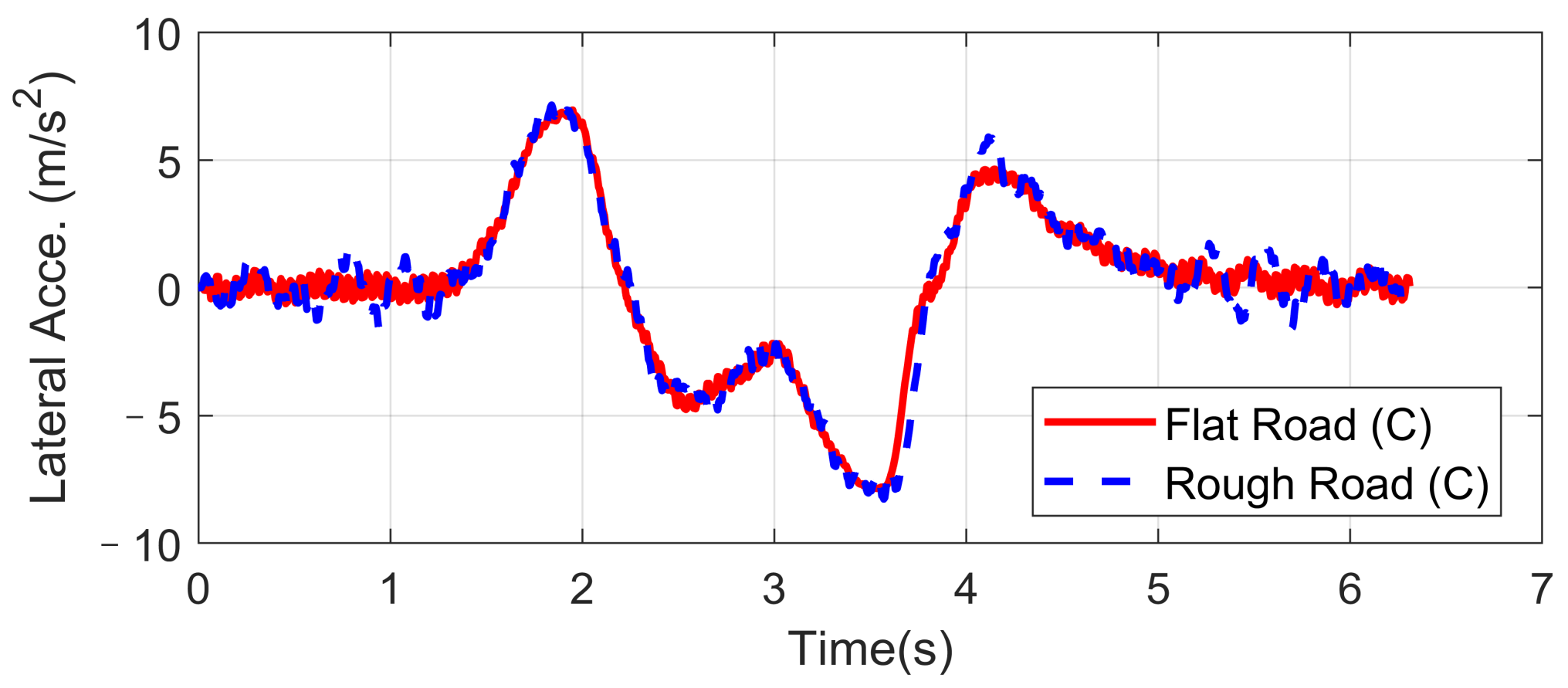
4.1. High-Speed Double Lane-Changing (DLC) on a Rough Road Surface

Double lane-changing is a standard test to evaluate the vehicle handling performance, which is usually done at a constant longitudinal speed. However, this maneuver becomes more challenging under a rough road surface at high speed because of the intensification of vertical vibration, and it is possible that the fluctuation of normal tire forces will influence the allocation accuracy of desired general longitudinal and lateral forces. In order to evaluate the dynamic performance of the proposed UCC system, a comparison simulation with the same controller was carried out based on the DLC test at 120 km/h speed under flat and rough road surfaces. The A-class uneven road profile is generated randomly. Since the effectiveness of active suspension control has been verified before, here we mainly focus on the lateral vehicle performances compared with the flat road situation. Simulations results are compared in Figure 9, Figure 10, Figure 11, Figure 12 and Figure 13.

The simulation verified that the CA method could generate desired resultant forces for the vehicle to complete the DLC maneuver under road roughness. Besides, the results in Figure 9, Figure 10 and Figure 11 demonstrate that the road disturbance generated slight undesired vehicle dynamics, including lateral and rolling motions. To investigate the effect of road roughness on the CA algorithm, the control values of the front left tire are compared in Figure 12 and Figure 13.

We can see from the results that the UCC method has a certain degree of robustness due to the sliding mode controller. However, in the critical points of DLC process (around 2 s and 3.5 s), the vehicle lateral acceleration and yaw rate approached their maximum values, and the tire forces were close to the boundary. In order to achieve the required lateral force, slip angles of four tires should not have a significant variation, as shown in Figure 12. In these critical time points, the normal force fluctuation led to an extra yaw moment, which is supposed to be compensated by the longitudinal vehicle forces. As can be seen in Figure 13, the tire slip variation in such time points was more significant than at other times, and this effect was even more severe in rough road conditions. Since in the proposed UCC strategy, the desired forces are evenly allocated into four tires, the situations of the other three tires were similar and will not be discussed to avoid redundant expression.

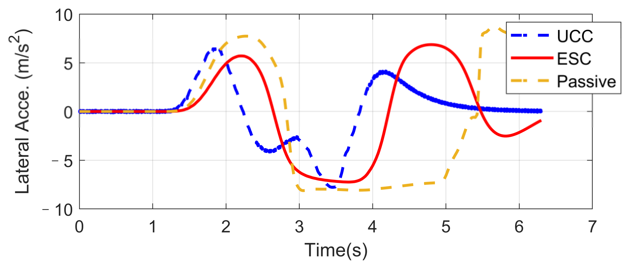
4.2. High-Speed Double Lane-Changing (DLC) on a Flat Road Surface (Compared with ESC)

Based on the same DLC test, while the first scenario examined the UCC performance on the uneven road, this second one focused on the comparison with the traditional ESC method. The ESC system is an envelope stability controller based on direct yaw control, which can only control the longitudinal force distribution among four tires. The results in Figure 14, Figure 15, Figure 16, Figure 17, Figure 18 and Figure 19 explain the superiority of the proposed UCC system on lateral vehicle dynamics compared with the ESC control strategy. The vehicle failed to pass this scenario without active control.

Figure 14, Figure 15 and Figure 16 and Figure 19 show yaw rate, vehicle slip angle, lateral acceleration, and vehicle path, respectively, and illustrate that the UCC has better performance than the ESC with respect to the yaw stability. Therein the desired vehicle slip angle control was well done by the UCC control. This is due to the fact that the vehicle system with multiple actuators can make full use of the adhesion coefficient of each wheel to generate desired resultant force/moment. By comparing the vehicle rolling and pitch angles presented in Figure 17 and Figure 18, one can clearly see that the proposed UCC maintained the body altitude effectively, enhancing the vehicle ride comfort due to active suspension control.

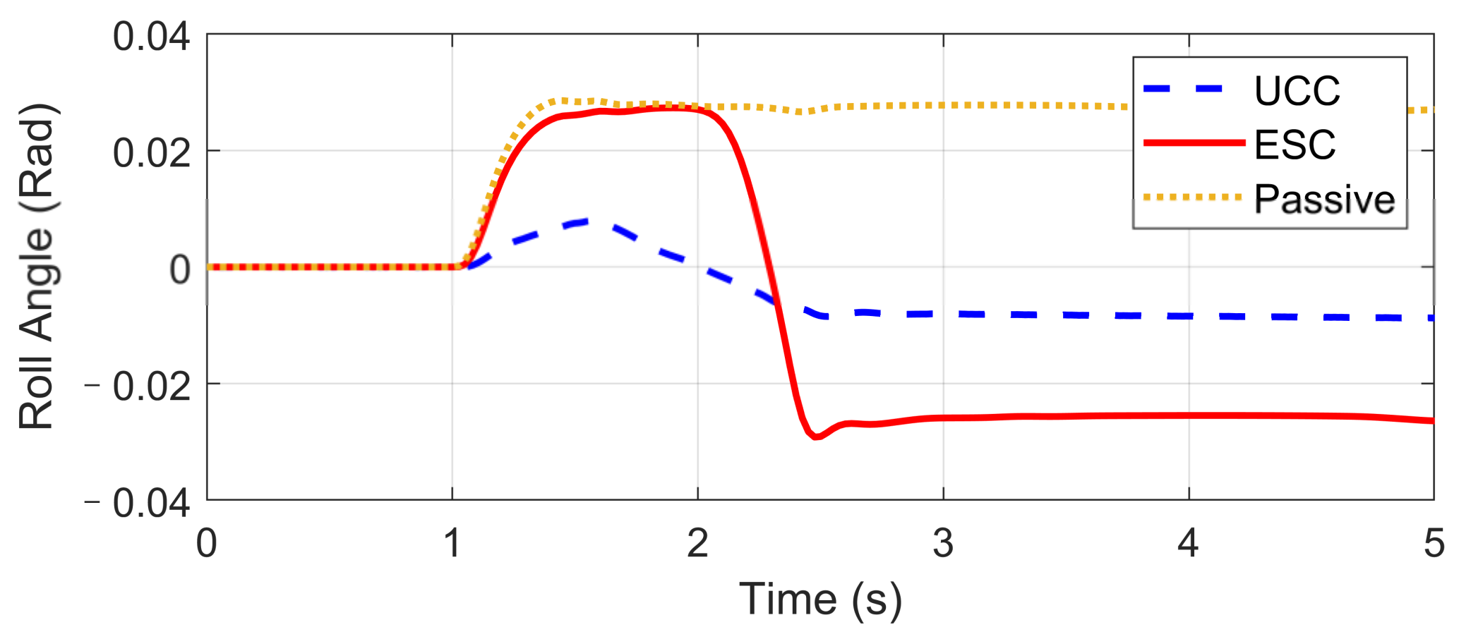
4.3. High-Speed Fishhook Maneuver

The Fishhook test is a dynamic test for predicting the dynamic rollover propensity. To begin the maneuver, the vehicle is driven in a straight line at the desired entrance speed, and then the driver releases the throttle and initiates the designed steering motion described in Figure 20. In this section, the steering maneuver of this test was adopted to verify the anti-rollover mechanism of the proposed UCC with the braking command triggered by the RI threshold set to 0.2. Figure 21, Figure 22, Figure 23, Figure 24 and Figure 25 shows the results at entrance speed 120 km/h concerning relative vehicle states. If no control strategy is applied, the vehicle will lose control early at around 1.5 s, as shown in the figures.

The result of vehicle RI clearly illustrates that, at time t = 1.5 and t = 2.3, when the steering angle reached its maximum value, the vehicle experienced the most apparent rollover propensity. Though the rollover did not happen actually due to the ESC control, the RI value still reached a dangerous level. The proposed UCC method can significantly reduce the RI value in the following two aspects.

(1)

The body altitude control function of UCC reduced the vehicle roll angle, indicated in Figure 23.

(2)

The braking force was triggered to inhibit the increase of lateral acceleration, which is shown in Figure 21.

We also observe from Figure 24 that the UCC method led to better dynamic performance and can achieve the desired yaw rate without losing stability. Additionally, the vehicle path curves shown in Figure 25 indicate that the undesired yaw moment generated by ESC control may promote the tendency of vehicle over-steering in high-speed curving situations, which can be avoided using the UCC with appropriate parameters tunning.

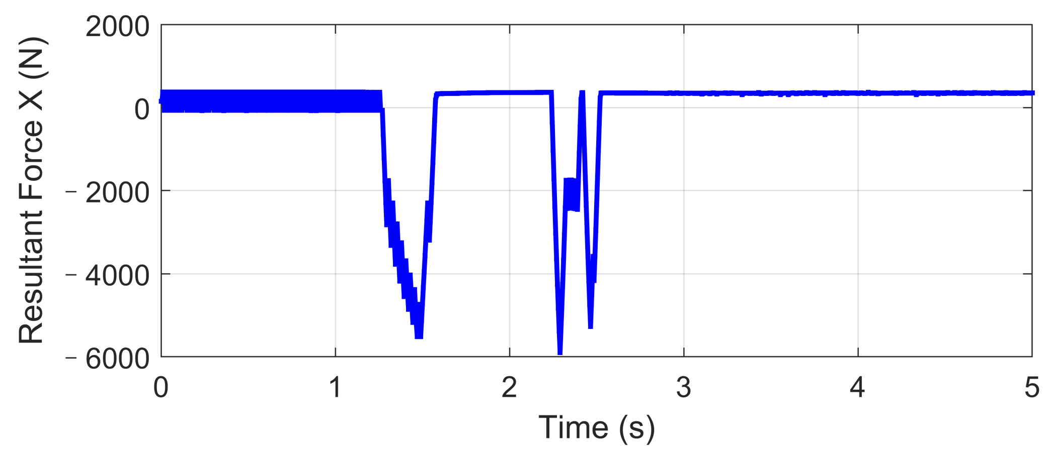
4.4. Tire Blow-Out in the Hard-Braking Process (Re-Configurable Control)

This scenario is designed for the condition where one tire blew out during hard braking. The initial vehicle speed is 120 km/h and a hard braking command (about −0.6 g) is given at 0 s, and then at the end of the first second, the front-left tire blew out and lost its lateral and longitudinal forces. The steering input is kept as zero, which keeps in line with the actual reaction. Based on different control strategies, three different conditions are considered, including UCC, ESC control, and passive vehicle. Results concerning vehicle and tire states are provided in Figure 26, Figure 27, Figure 28, Figure 29 and Figure 30.

Curves in Figure 26 and Figure 27 described the re-allocation of tire longitudinal and lateral forces (in the body coordinate) after the front-left tire blew out through a reconfigurable UCC approach, keeping the desired resultant forces/moment unchanged. The vehicle yaw rate and path based on different control configurations are shown in Figure 28 and Figure 29. These results illustrate the extra yaw moment due to the tire blowing-out and the lane departure behavior it caused for both the ESC control and passive situations. However, the prompt intervention of driver steering input (closed-loop ESC in figures) can reduce the danger to some extent accompanied by ESC, but it is highly demanding for non-professional drivers to respond appropriately under such emergencies.

On the contrary, the UCC just required the driver to keep straight ahead. Additionally, it is worth noticing in Figure 30 that the traditional ESC control cannot compensate for the lost tire brake forces. Thus, the brake distance was increased. However, the UCC reconfigurable method was able to hold the initial braking deceleration and inhibit the interference of extra yaw moment due to the re-allocation of tire forces. The proposed UCC is the only strategy that is able to keep the driver’s intention for this emergency.

5. Conclusions

In this paper, a UCC strategy involving the vehicle yaw stability, body altitude, and tire contact stability was presented. A hierarchical control structure was adopted to realize the UCC, including high-level sliding mode control, fixed point CA, and a normal tire force robust tracking controller. Simulations of high-demanding driving situations concerning rough road surface, fast DLC, fishhook maneuver, and the tire blowing-out situation performed on a nonlinear full vehicle model have shown the effectiveness and advantages of the proposed control method. The following conclusions can be drawn:

(1)

For a four-wheel independent drive–independent steering configuration, the proposed UCC method can effectively realize the tire planar force distribution and the desired vehicle motion, which proves to be a practical solution due to its simple feedback control rules and reconfigurable allocation.

(2)

Considering the wheel vertical vibrations, we present a robust tire normal force tracking controller to address the tire contact stability issue. This work provides an innovative method for improving the vehicle driving stability and maintaining the desired body attitude simultaneously.

References

1. Murata, S. Innovation by in-wheel-motor drive unit. Veh. Syst. Dyn. 2012, 50, 807–830. [Google Scholar] [CrossRef]
2. Koehn, P.; Eckrich, M. Active steering-the BMW approach towards modern steering technology. SAE Tech. Pap. 2004. [Google Scholar] [CrossRef]
3. Gysen, B.L.; Paulides, J.J.; Janssen, J.L.; Lomonova, E.A. Active electromagnetic suspension system for improved vehicle dynamics. IEEE Trans. Veh. Technol. 2010, 59, 1156–1163. [Google Scholar] [CrossRef] [Green Version]
4. Hoehn, B.R.; Stahl, K.; Gwinner, P.; Wiesbeck, F. Torque-vectoring driveline for electric vehicles. In Proceedings of the International Federation of Automotive Engineering Societies FISITA 2012 World Automotive Congress; Springer: Berlin/Heidelberg, Germany, 2013; pp. 585–593. [Google Scholar] [CrossRef]
5. Bouvin, J.L.; Hamrouni, E.; Moreau, X.; Benine-Neto, A.; Hernette, V.; Serrier, P.; Oustaloup, A. Hierarchical approach for global chassis control. In Proceedings of the 2018 European Control Conference (ECC), Limassol, Cyprus, 12–15 June 2018; pp. 2555–2560. [Google Scholar] [CrossRef]
6. Vivas-Lopez, C.A.; Tudon-Martinez, J.C.; Hernandez-Alcantara, D.; Morales-Menendez, R. Global chassis control system using suspension, steering, and braking subsystems. Math. Probl. Eng. 2015, 2015, 263424. [Google Scholar] [CrossRef] [Green Version]
7. Chokor, A.; Talj, R.; Doumiati, M.; Charara, A. A global chassis control system involving active suspensions, direct yaw control and active front steering. IFAC-PapersOnLine 2019, 52, 444–451. [Google Scholar] [CrossRef]
8. Cho, W.; Yoon, J.; Kim, J.; Hur, J.; Yi, K. An investigation into unified chassis control scheme for optimised vehicle stability and manoeuvrability. Veh. Syst. Dyn. 2008, 46, 87–105. [Google Scholar] [CrossRef]
9. Cho, W.; Choi, J.; Kim, C.; Choi, S.; Yi, K. Unified chassis control for the improvement of agility, maneuverability, and lateral stability. IEEE Trans. Veh. Technol. 2012, 61, 1008–1020. [Google Scholar] [CrossRef]
10. Yoon, J.; Cho, W.; Koo, B.; Yi, K. Unified chassis control for rollover prevention and lateral stability. IEEE Trans. Veh. Technol. 2009, 58, 596–609. [Google Scholar] [CrossRef]
11. Poussot-Vassal, C.; Sename, O.; Dugard, L.; Savaresi, S.M. Vehicle dynamic stability improvements through gain-scheduled steering and braking control. Veh. Syst. Dyn. 2011, 49, 1597–1621. [Google Scholar] [CrossRef] [Green Version]
12. He, J.; Crolla, D.A.; Levesley, M.C.; Manning, W.J. Coordination of active steering, driveline, and braking for integrated vehicle dynamics control. Proc. Inst. Mech. Eng. Part D J. Automob. Eng. 2006, 220, 1401–1420. [Google Scholar] [CrossRef]
13. Ono, E.; Hattori, Y.; Muragishi, Y.; Koibuchi, K. Vehicle dynamics integrated control for four-wheel-distributed steering and four-wheel-distributed traction/braking systems. Veh. Syst. Dyn. 2006, 44, 139–151. [Google Scholar] [CrossRef]
14. Zhao, J.; Wong, P.K.; Ma, X.; Xie, Z. Chassis integrated control for active suspension, active front steering and direct yaw moment systems using hierarchical strategy. Veh. Syst. Dyn. 2017, 55, 72–103. [Google Scholar] [CrossRef]
15. Mousavinejad, E.; Han, Q.L.; Yang, F.; Zhu, Y.; Vlacic, L. Integrated control of ground vehicles dynamics via advanced terminal sliding mode control. Veh. Syst. Dyn. 2017, 55, 268–294. [Google Scholar] [CrossRef]
16. Cheng, S.; Li, L.; Liu, C.Z.; Wu, X.; Fang, S.N.; Yong, J.W. Robust LMI-Based H-Infinite Controller Integrating AFS and DYC of Autonomous Vehicles with Parametric Uncertainties. IEEE Trans. Syst. Man Cybern. Syst. 2020. [Google Scholar] [CrossRef]
17. Sun, J.; Cong, J.; Gu, L.; Dong, M. Fault-tolerant control for vehicle with vertical and lateral dynamics. Proc. Inst. Mech. Eng. Part D J. Automob. Eng. 2019, 233, 3165–3184. [Google Scholar] [CrossRef]
18. Wang, R.; Wang, J. Fault-tolerant control for electric ground vehicles with independently-actuated in-wheel motors. J. Dyn. Syst. Meas. Control. 2012, 134. [Google Scholar] [CrossRef]
19. Ataei, M.; Khajepour, A.; Jeon, S. Model Predictive Control for integrated lateral stability, traction/braking control, and rollover prevention of electric vehicles. Veh. Syst. Dyn. 2020, 58, 49–73. [Google Scholar] [CrossRef]
20. Guo, J.; Luo, Y.; Li, K.; Dai, Y. Coordinated path-following and direct yaw-moment control of autonomous electric vehicles with sideslip angle estimation. Mech. Syst. Signal Process. 2018, 105, 183–199. [Google Scholar] [CrossRef]
21. Peng, H.; Wang, W.; An, Q.; Xiang, C.; Li, L. Path tracking and direct yaw moment coordinated control based on robust MPC with the finite time horizon for autonomous independent-drive vehicles. IEEE Trans. Veh. Technol. 2020, 69, 6053–6066. [Google Scholar] [CrossRef]
22. Pylypchuk, V.; Chen, S.K.; Moshchuk, N.; Litkouhi, B. Slip-Based Holistic Corner Control. In Proceedings of the ASME 2011 International Mechanical Engineering Congress and Exposition, Denver, CO, USA, 11–17 November 2011; pp. 337–342. [Google Scholar] [CrossRef]
23. Chen, S.K.; Ghoneim, Y.; Moshchuk, N.; Litkouhi, B.; Pylypchuk, V. Tire-Force Based Holistic Corner Control. In Proceedings of the ASME 2012 International Mechanical Engineering Congress and Exposition, Volume 11: Transportation Systems, Houston, TX, USA, 9–15 November 2012; pp. 133–140. [Google Scholar] [CrossRef]
24. Wang, J.; Longoria, R.G. Coordinated and reconfigurable vehicle dynamics control. IEEE Trans. Control. Syst. Technol. 2009, 17, 723–732. [Google Scholar] [CrossRef]
25. Shim, T.; Margolis, D. Dynamic normal force control for vehicle stability enhancement. Int. J. Veh. Auton. Syst. 2005, 3, 1–14. [Google Scholar] [CrossRef]
26. Gáspár, P.; Szabó, Z.; Bokor, J. The design of an integrated control system in heavy vehicles based on an LPV method. In Proceedings of the 44th IEEE Conference on Decision and Control, Seville, Spain, 12–15 December 2005; pp. 6722–6727. [Google Scholar] [CrossRef] [Green Version]
27. Poussot-Vassal, C.; Sename, O.; Dugard, L.; Gaspar, P.; Szabo, Z.; Bokor, J. Attitude and handling improvements through gain-scheduled suspensions and brakes control. Control. Eng. Pract. 2011, 19, 252–263. [Google Scholar] [CrossRef] [Green Version]
28. Hrovat, D. Influence of unsprung weight on vehicle ride quality. J. Sound Vib. 1988, 124, 497–516. [Google Scholar] [CrossRef]
29. Besselink, I.J.M.; Vos, R.; Nijmeijer, H. Influence of in-wheel motors on the ride comfort of electric vehicles. In Proceedings of the 10th International Symposium on Advanced Vehicle Control (AVEC10), Loughborough, UK, 22–26 August 2010; pp. 835–840. [Google Scholar]
30. Zhang, L.; Li, L.; Qi, B. Rollover prevention control for a four in-wheel motors drive electric vehicle on an uneven road. Sci. China Technol. Sci. 2018, 61, 934–948. [Google Scholar] [CrossRef]
31. Tan, D.; Wang, H.; Wang, Q. Study on the rollover characteristic of in-wheel-motor-driven electric vehicles considering road and electromagnetic excitation. Shock Vib. 2016, 2016, 1–13. [Google Scholar] [CrossRef]
32. Pacejka, H.B.; Bakker, E. The magic formula tyre model. Veh. Syst. Dyn. 1992, 21, 1–18. [Google Scholar] [CrossRef]
33. Hurel, J.; Mandow, A.; García-Cerezo, A. Kinematic and dynamic analysis of the McPherson suspension with a planar quarter-car model. Veh. Syst. Dyn. 2013, 51, 1422–1437. [Google Scholar] [CrossRef]
34. Wang, W.; Chen, X.; Wang, J. Unsprung Mass Effects on Electric Vehicle Dynamics based on Coordinated Control Scheme. In Proceedings of the 2019 American Control Conference (ACC), Philadelphia, PA, USA, 10–12 July 2019; pp. 971–976. [Google Scholar] [CrossRef]
35. Doyle, J.; Glover, K.; Khargonekar, P.; Francis, B. State-space solutions to standard H2 and H∞ control problems. In Proceedings of the 1988 American Control Conference, Atlanta, GA, USA, 15–17 June 1988; pp. 1691–1696. [Google Scholar] [CrossRef] [Green Version]
Figure 2. Vehicle roll and pitch motion.
Sensors 21 03931 g002
Figure 3. The architecture of unified vehicle dynamics control.
Sensors 21 03931 g003
Figure 4. One-fourth active suspension model with body inertia force.
Sensors 21 03931 g004
Figure 5. Robust tracking control of tire contact force.
Sensors 21 03931 g005
Figure 7. Performance of Controllers 1 and 2: (a) body acceleration; (b) tire dynamic load.
Sensors 21 03931 g007
Figure 8. Normal force tracking of controller 2.
Sensors 21 03931 g008
Figure 9. Lateral acceleration in high-speed DLC.
Sensors 21 03931 g009
Figure 10. Vehicle slip angle in high-speed DLC.
Sensors 21 03931 g010
Figure 11. Rollover index in high-speed DLC.
Sensors 21 03931 g011
Figure 12. FL tire slip in high-speed DLC.
Sensors 21 03931 g012
Figure 13. FL tire slip angle in high-speed DLC.
Sensors 21 03931 g013
Figure 14. Yaw rate on flat road during high-speed DLC.
Sensors 21 03931 g014
Figure 15. Vehicle slip angle on flat road during high-speed DLC.
Sensors 21 03931 g015
Figure 16. Lateral acceleration on flat road during high-speed DLC.
Sensors 21 03931 g016
Figure 17. Body roll angle on flat road during high-speed DLC.
Sensors 21 03931 g017
Figure 18. Body pitch angle on flat road during high-speed DLC.
Sensors 21 03931 g018
Figure 19. Vehicle path on flat road during high-speed DLC.
Sensors 21 03931 g019
Figure 20. Steering angle in high-speed fishhook maneuver.
Sensors 21 03931 g020
Figure 21. Longitudinal force in high-speed fishhook maneuver.
Sensors 21 03931 g021
Figure 22. Rollover index in high-speed fishhook maneuver.
Sensors 21 03931 g022
Figure 23. Body roll angle in high-speed fishhook maneuver.
Sensors 21 03931 g023
Figure 24. Yaw rate in high-speed fishhook maneuver.
Sensors 21 03931 g024
Figure 25. Vehicle global path in high-speed fishhook maneuver.
Sensors 21 03931 g025
Figure 26. Longitudinal force in hard-braking.
Sensors 21 03931 g026
Figure 27. Lateral force in hard-braking.
Sensors 21 03931 g027
Figure 28. Yaw rate in hard-braking.
Sensors 21 03931 g028
Figure 29. Vehicle path in hard-braking.
Sensors 21 03931 g029
Figure 30. Vehicle speed in hard-braking.
Sensors 21 03931 g030