
Wavefront Restoration Technology of Dynamic Non-Uniform Intensity Distribution Based on Extreme Learning Machine


Abstract
:1. Introduction
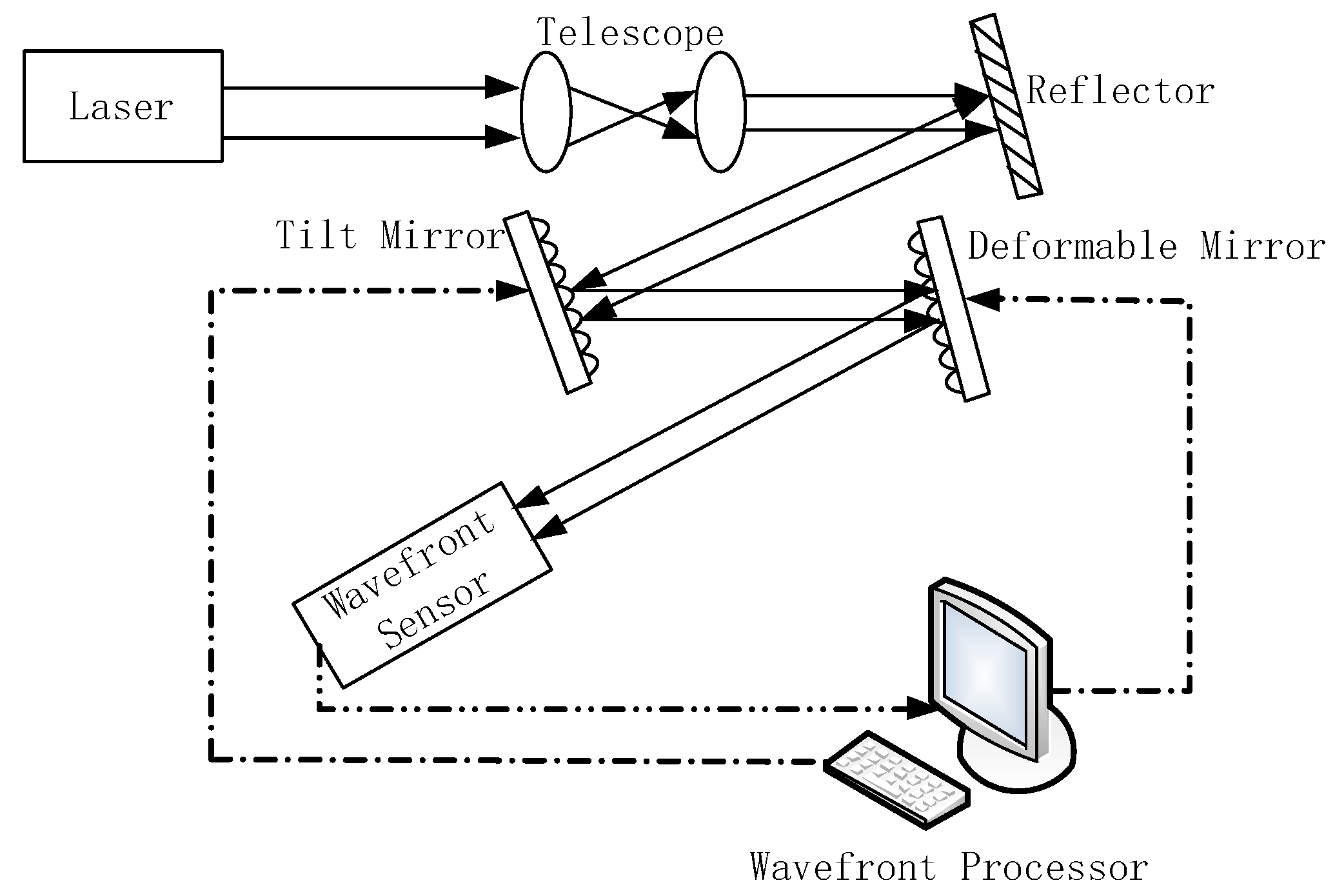
2. Principle
3. Numerical Simulations
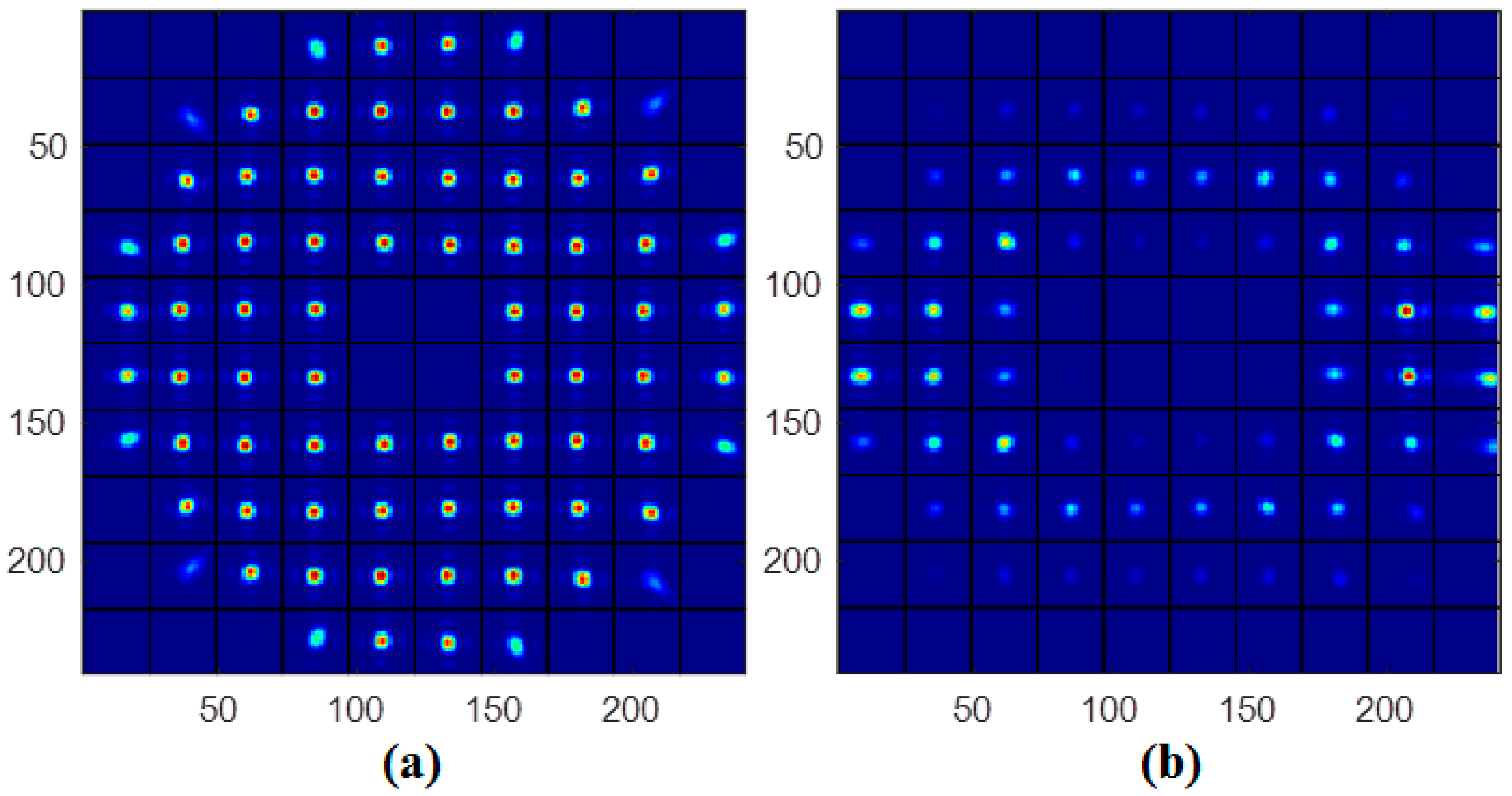
3.1. Dataset
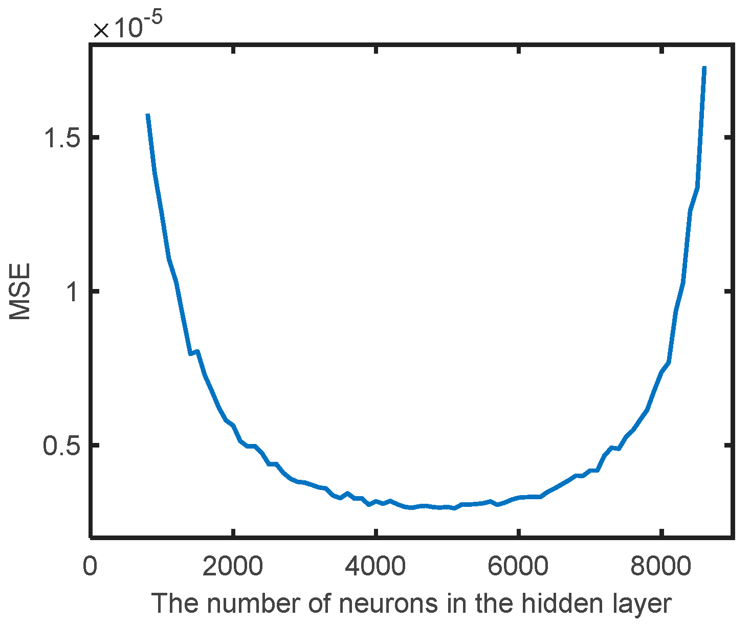
3.2. Model Training and Optimization
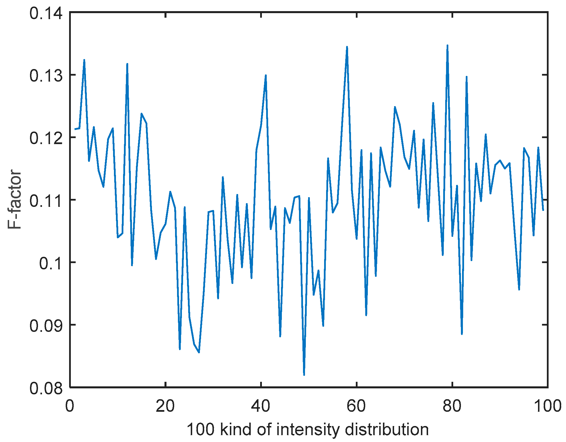
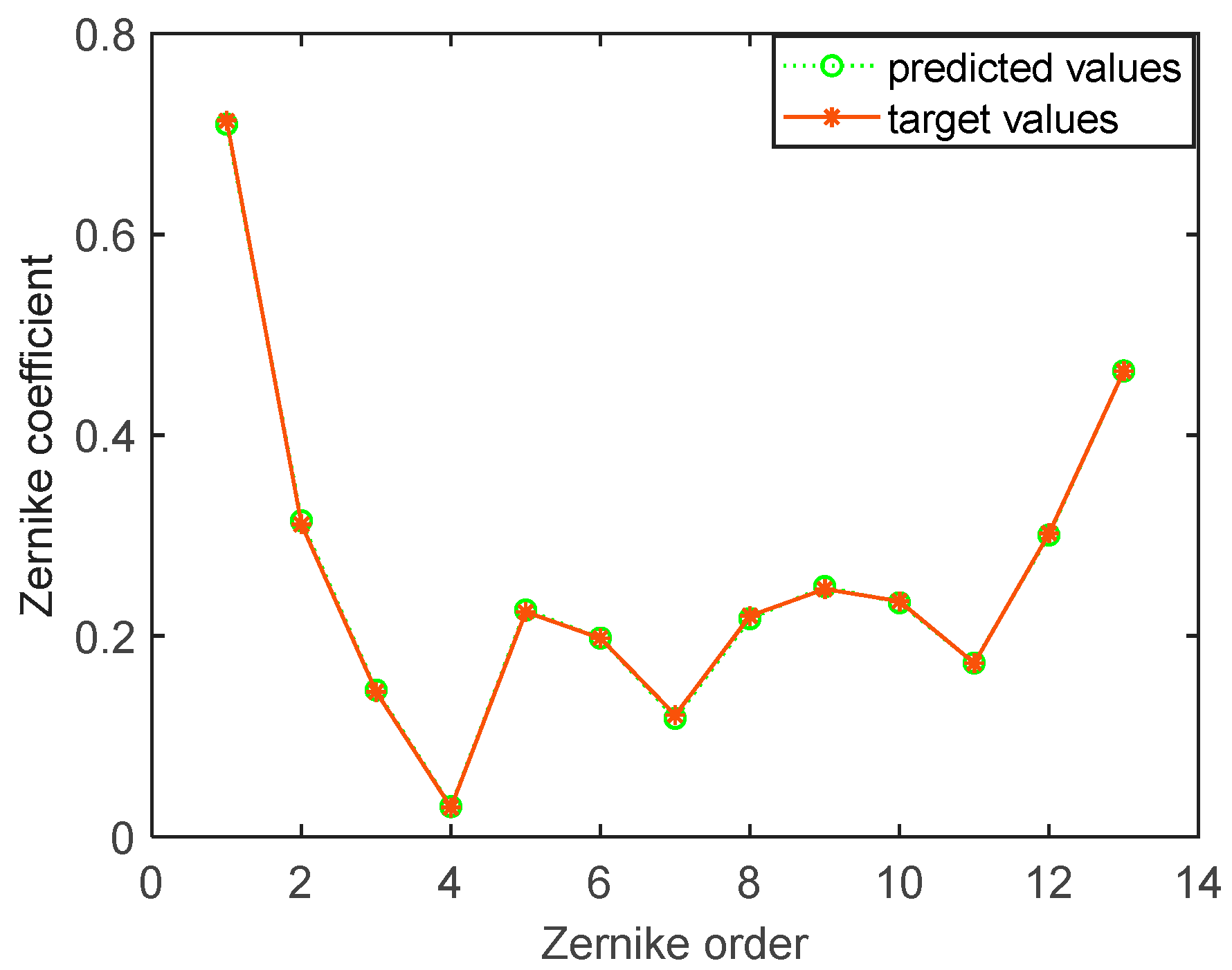
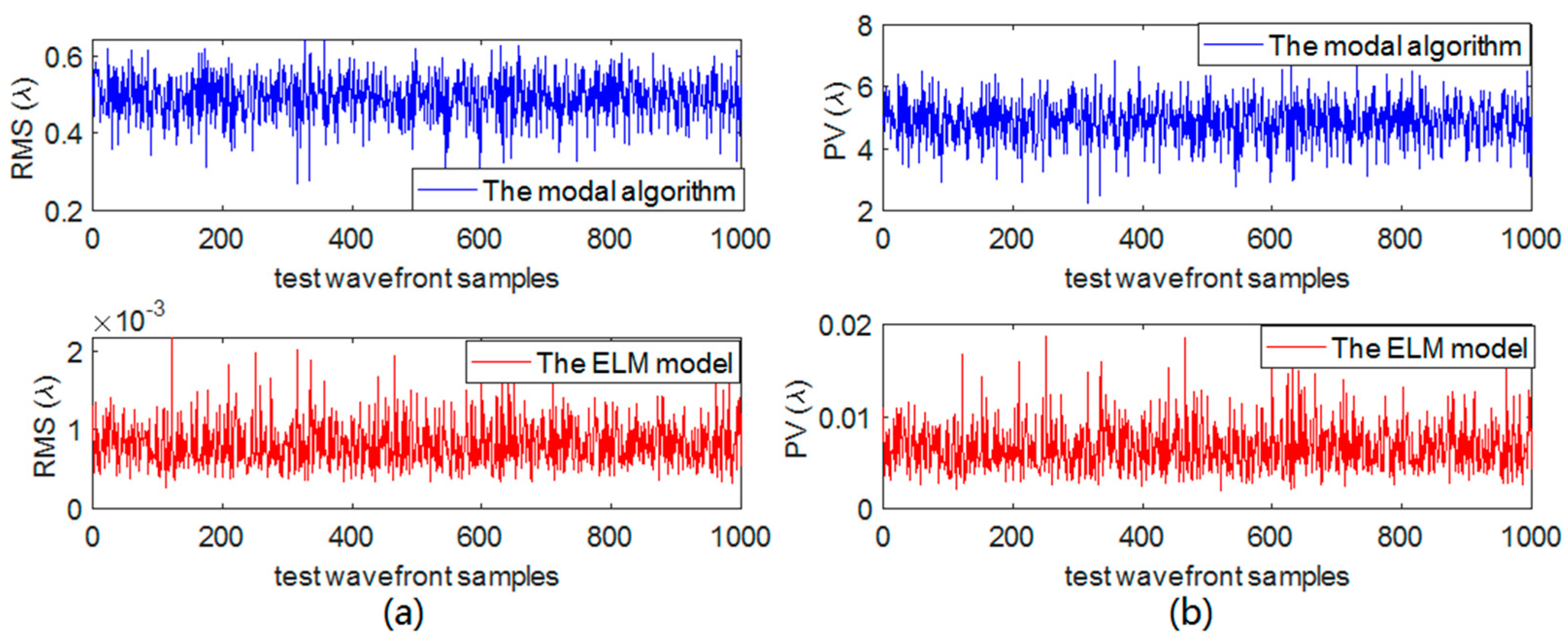
3.3. Prediction Results
4. Conclusions
Author Contributions
Funding
Institutional Review Board Statement
Informed Consent Statement
Conflicts of Interest
References
- Numata, K.; Riris, H.; Li, S.; Wu, S.; Kawa, S.R.; Krainak, M.; Abshire, J. Ground demonstration of trace gas lidar based on optical parametric amplifier. J. Appl. Remote Sens. 2012, 6, 063561. [Google Scholar] [CrossRef]
- Walsh, B.M.; Lee, H.R.; Barnes, N.P. Mid infrared lasers for remote sensing applications. J. Lumin. 2016, 169, 400–405. [Google Scholar] [CrossRef]
- Mackanos, M.A.; Simanovskii, D.M.; Schriver, K.E.; Hutson, M.S.; Contag, C.H.; Kozub, J.A.; Jansen, E.D. Pulse-duration-dependent mid-infrared laser ablation for biological applaications. IEEE J. Sel. Top. Quantum Electron. 2012, 18, 1514–1522. [Google Scholar] [CrossRef]
- Jackson, S.D. Towards high-power mid infrared emission from a fiber laser. Nat. Photonics 2012, 6, 423–431. [Google Scholar] [CrossRef]
- Liu, J.; Chen, X.; Xinyu, C.; Wu, C.; Bai, F.; Jin, G. Analytical solution of the thermal effects in a high-power slab Tm:YLF laser with dual-end pumping. Phys. Rev. A 2016, 93, 013854. [Google Scholar] [CrossRef]
- Scaggs, M.; Haas, G. Thermal lensing compensation optics for high power lasers. Proc. SPIE 2011, 7913, 79130C. [Google Scholar]
- Yang, P.; Ning, Y.; Lei, X.; Xu, B.; Li, X.; Dong, L.; Yan, H.; Liu, W.; Jiang, W.; Liu, L.; et al. Enhancement of the beam quality of non-uniform output slab laser amplifier with a 39-actuator rectangular piezoelectric deformable mirror. Opt. Express 2010, 18, 7121–7130. [Google Scholar] [CrossRef]
- Patel, F.D.; Harris, D.G.; Turner, J.C.E. Improving the beam quality of a high power Yb: YAG rod laser. Proc. SPIE 2006, 6100, 610018–610021. [Google Scholar]
- Wittrock, U.; Bostanjoglo, G.; Dong, S.; Eppich, B.; Haase, T.; Lue, Q.; Mueller-Stolzenburg, N.; Holst, O. High-power solid state lasers with improved beam quality. Proc. SPIE 1994, 2206, 396–407. [Google Scholar]
- Yu, X.; Dong, L.; Lai, B.; Yang, P.; Liu, Y.; Kong, Q.; Yang, K.; Tang, G.; Xu, B. Automatic low-order aberration correction based on geometrical optics for slab laser. Appl. Opt. 2017, 56, 1730–1739. [Google Scholar] [CrossRef]
- Lei, X.L.X.; Xu, B.X.B.; Yang, P.Y.P.; Dong, L.D.L.; Liu, W.L.W.; Yan, H.Y.H. Beam cleanup of a532-nm pulsed solid-state laser using a bimorph mirror. Chin. Opt. Lett. 2012, 10, 021401–021404. [Google Scholar]
- Yang, P.; Liu, Y.; Ao, M.W.; Hu, S.J.; Xu, B. A wavefront sensor-less adaptive optical system for a solid-state lase. Opt. Commun. 2007, 278, 377–381. [Google Scholar] [CrossRef]
- Fourmaux, S.; Serbanescu, C.; Lecherbourg, L.; Payeur, S.; Martin, F.; Kieffer, J.C. Characterization of the laser beam distortion due to the thermal load on high average power femtosecond laser systems. Proc. SPIE 2009, 7386, 738637. [Google Scholar]
- Rothhardt, J.; Demmler, S.; Hädrich, S.; Peschel, T.; Limpert, J.; Tünnermann, A. Thermal effects in high average power optical parametric amplifiers. Opt. Lett. 2013, 38, 763. [Google Scholar] [CrossRef] [PubMed]
- Xu, Z.; Wang, S.; Zhao, M.; Zhao, W.; Dong, L.; He, X.; Yang, P.; Xu, B.; Zhiqiang, X.; Mengmeng, Z.; et al. Wavefront reconstruction of a Shack–Hartmann sensor with insufficient lenslets based on an extreme learning machine. Appl. Opt. 2020, 59, 4768–4774. [Google Scholar] [CrossRef]
- Barwick, S. Detecting higher-order wavefront errors with an astigmatic hybrid wavefront sensor. Opt. Lett. 2009, 34, 1690–1692. [Google Scholar] [CrossRef] [PubMed]
- Guo, H.; Korablinova, N.; Ren, Q.; Bille, J. Wavefront reconstruction with artificial neural networks. Opt. Express 2006, 14, 6456–6462. [Google Scholar] [CrossRef] [PubMed]
- Li, Z.; Li, X. Centroid computation for Shack-Hartmann wavefront sensor in extreme situations based on artificial neural networks. Opt. Express 2018, 26, 31675–31692. [Google Scholar] [CrossRef]
- Hu, L.J.; Hu, S.W.; Gong, W.; Si, K. Learning-based ShackHartmann wavefront sensor for high-order aberration detection. Opt. Express 2019, 27, 33504–33517. [Google Scholar] [CrossRef]
- Huang, G.; Huang, G.B.; Song, S.; You, K. Trends in extreme learning machines: A review. Neural Netw. 2015, 61, 32–48. [Google Scholar] [CrossRef]
- Huang, G.-B.; Zhu, Q.-Y.; Siew, C.-K. Extreme learning machine: Theory and applications. Neurocomputing 2006, 70, 489–501. [Google Scholar] [CrossRef]
- Zhu, Q.Y.; Qin, A.K.; Suganthan, P.N.; Huang, G.B. Evolutionary exetreme learning machine. Pattern Recognit. 2005, 38, 1759–1763. [Google Scholar] [CrossRef]
- Feng, G.; Huang, G.-B.; Lin, Q.; Gay, R. Error Minimized Extreme Learning Machine with Growth of Hidden Nodes and Incremental Learning. IEEE Trans. Neural Netw. 2009, 20, 1352–1357. [Google Scholar] [CrossRef] [PubMed]
- Noll, R.J. Phase estimates from slope-type wave-front sensors. J. Opt. Soc. Am. 1978, 68, 139–140. [Google Scholar] [CrossRef]


| Parameters | Value |
|---|---|
| Wavelength | 1064 nm |
| Numbers of micro-lens | 10 × 10 |
| Focal length of micro-lens | 21.7 mm |
| Valid sub-aperture | 76 |
| Numbers of pixel in each sub-aperture | 24 × 24 pixels |
| Pixel size | 14 μm |
| Sampling frequency of WFS camera | 1000 Hz |
| Activation Function | MSE |
|---|---|
| softplus | 2.9489 × 10⁻⁶ |
| Relu | 2.6361 × 10⁻⁵ |
| sig | 7.5124 × 10⁻⁵ |
| tanh | 4.3081 × 10⁻⁴ |
| sin | 0.0024 |
| hardlim | 0.0015 |
| RBF | 0.0110 |
Publisher’s Note: MDPI stays neutral with regard to jurisdictional claims in published maps and institutional affiliations. |
© 2021 by the authors. Licensee MDPI, Basel, Switzerland. This article is an open access article distributed under the terms and conditions of the Creative Commons Attribution (CC BY) license (https://creativecommons.org/licenses/by/4.0/).
Share and Cite
Lin, H.; He, X.; Wang, S.; Yang, P. Wavefront Restoration Technology of Dynamic Non-Uniform Intensity Distribution Based on Extreme Learning Machine. Sensors 2021, 21, 3877. https://doi.org/10.3390/s21113877
Lin H, He X, Wang S, Yang P. Wavefront Restoration Technology of Dynamic Non-Uniform Intensity Distribution Based on Extreme Learning Machine. Sensors. 2021; 21(11):3877. https://doi.org/10.3390/s21113877
Chicago/Turabian StyleLin, Haiqi, Xing He, Shuai Wang, and Ping Yang. 2021. "Wavefront Restoration Technology of Dynamic Non-Uniform Intensity Distribution Based on Extreme Learning Machine" Sensors 21, no. 11: 3877. https://doi.org/10.3390/s21113877
APA StyleLin, H., He, X., Wang, S., & Yang, P. (2021). Wavefront Restoration Technology of Dynamic Non-Uniform Intensity Distribution Based on Extreme Learning Machine. Sensors, 21(11), 3877. https://doi.org/10.3390/s21113877