Abstract
In control and monitoring of manufacturing processes, it is key to understand model uncertainty in order to achieve the required levels of consistency, quality, and economy, among others. In aerospace applications, models need to be very precise and able to describe the entire dynamics of an aircraft. In addition, the complexity of modern real systems has turned deterministic models impractical, since they cannot adequately represent the behavior of disturbances in sensors and actuators, and tool and machine wear, to name a few. Thus, it is necessary to deal with model uncertainties in the dynamics of the plant by incorporating a stochastic behavior. These uncertainties could also affect the effectiveness of fault diagnosis methodologies used to increment the safety and reliability in real-world systems. Determining suitable dynamic system models of real processes is essential to obtain effective process control strategies and accurate fault detection and diagnosis methodologies that deliver good performance. In this paper, a maximum likelihood estimation algorithm for the uncertainty modeling in linear dynamic systems is developed utilizing a stochastic embedding approach. In this approach, system uncertainties are accounted for as a stochastic error term in a transfer function. In this paper, we model the error-model probability density function as a finite Gaussian mixture model. For the estimation of the nominal model and the probability density function of the parameters of the error-model, we develop an iterative algorithm based on the Expectation-Maximization algorithm using the data from independent experiments. The benefits of our proposal are illustrated via numerical simulations.
1. Introduction
System identification is a scientific discipline that studies techniques for modeling and estimating dynamic systems from experimental data, i.e., a number of experiments are performed on the system, and a model is then fitted to the measured data by estimating the corresponding system model parameters [1,2]. Most system identification techniques available in the literature assume that the system model that will be fitted lies in the model set [3]. However, real processes have an arbitrary complexity and using a complex model structure can lead to large variance estimation errors [4]. Moreover, the experimental data is typically obtained with the presence of sensors errors and measurement noise, modeling errors, and external disturbances that can impact on the system model accuracy; see, e.g., Reference [5]. This scenario has been considered for sensor or actuator failure diagnosis and isolation in systems with structural uncertainties and noisy measurements, utilizing residual analysis and Bayesian frameworks to develop failure detection procedures [6,7,8,9].
In Figure 1, a typical representation of a real process and measured experimental data is shown, where is the input measurements, denotes the output measurements, and denotes a measurement noise. The real process (true system) is represented by the interaction of three components: (i) an actuator, (ii) a plant, and (iii) a sensor. This representation has been used to develop system identification methodologies for flight vehicle development in order to obtain accurate models and to validate mathematical models of the flight vehicle [10]. These system models are required, for example, to perform fault-diagnosis and adaptive control, to analyze handling qualities specification compliance, to develop high-fidelity aerodynamic databases for flight simulators, among others [11]. However, the quality of these results can be affected by the uncertainties incorporated by the (unknown) dynamics that are not modeled, the instrumentation, model simplifications, and measurement noise and sensor errors [12].
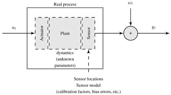
Figure 1.
Representation of a real dynamic system with data measurements for system identification.
On the other hand, in Reference [13], the modeling and parameter identification in structural health monitoring was addressed. The authors considered that the multi-sensor data in a structural health monitoring can provide incomplete information due to multi-sensor faults or errors and then quantified its corresponding uncertainty with a Bayesian framework. Similarly, in Reference [14], a sensor-orientated approach for space situational awareness and traffic management uncertainty quantification was presented, analyzing the implications of the sensor uncertainties in the performance of this systems. A mathematical formulation based on the least square method was developed, providing a methodology to represent the navigation and tracking errors as an uncertainty volume that accurately depicts the size and orientation in space situational awareness evolution.
For these reasons, a suitable formulation of a model that incorporates uncertainties is an important aspect to consider in system identification methods, in order to obtain system models that represent as closely as possible the real process behavior [1,2,10]. Because of its valuable statistical properties [1,2,3], many identification algorithms involve the maximum likelihood (ML) principle with particular system models, such as dynamic systems [15,16,17], static systems [18], systems with quantized output data [19,20,21,22], and communications [23,24], to mention a few. In particular, the ML estimators are asymptotically unbiased. That is, when the number of measurements is not too large, the estimates can be far from the true value. This bias is typically accounted for by the measurement noise variance. However, there are scenarios in which the number of sampled-data is, in theory, large enough, and the estimates considerably change from one experiment to another, i.e., there is an uncertainty in the system model that cannot be accounted for by the noise measurements and a large variance.
To illustrate the stochastic embedding approach, the magnitude of the frequency response of a linear dynamic system (assumed to be the true system) is shown in Figure 2, where is given by
where denotes the backward shift operator (), r denotes a realization of the true system, is a fixed nominal model, and denotes the rth realization of a relative error-model for the true system. The red-shaded region represents the area in which possible true systems, , i.e, realizations of the true system (represented by black dotted lines), can lie. The error-model can introduce model parameter uncertainties at low frequency range and model structure uncertainties at high frequency range [10]. This system model behavior can be encountered, for instance, in an aeroservoelastic system model (see, e.g., References [5,25]). Aeroservoelastic systems include dynamic coupling due to structural, control, sensor and actuator dynamics that cover both the low frequency and high frequency range. This means that, in an ML framework, the estimates can change considerable from one experiment to another, even if the number of measurements used to obtain an ML estimation is large, due to the structural and parametric uncertainties in the true system model. Hence, it is desirable that the models obtained from system identification techniques provide a quantification of their uncertainty, i.e., considering that the uncertainty modeling is part of the structure and estimating a nominal model with an error-model [26,27,28]. This approach of uncertainty modeling can be used for robust control design in which optimization methods can be used to obtain controllers in order to minimize the expected variation (variance) of the true system performance from a given desired behavior [29], or to obtain a probabilistic solution for robust control design [30,31].
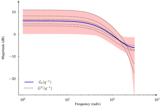
Figure 2.
Magnitude of the frequency response for the linear dynamic system in Equation (1).
This alternative view of modeling error-model has been addressed in different frameworks. In Reference [32], the set membership approach was used to deal with the problem of uncertainty modeling in dynamic systems. The authors of Reference [32] considered the error-model estimation in a deterministic framework in which it is unknown-but-bounded and obtaining a set of possible solutions. However, this method does not guarantee a small set of solutions to properly describe the system model uncertainty. In Reference [33], classical prediction error methods (PEM) [2] were used to obtain an estimation of the nominal model. Then, the unmodeled dynamics were estimated from the residuals dynamics using PEM and obtaining the corresponding model error modeling (MEM). Nevertheless, this methodology assumes that the nominal model is available. In References [26,34], a stochastic embedding (SE) approach was used to describe the model uncertainty by considering the model as a realization drawn from an underlying probability space, where the parameters that define the error-model are characterized by a probability density function (PDF). However, a flexible error-model distribution is needed to obtain a correct description of the system model uncertainty. In this approach, the uncertainty can be quantified by using ML estimation considering the parameters of the error-model as hidden variables [4,35] and solving the associated estimation problem with an expectation-maximization (EM) [36] based algorithm under Gaussian assumptions for the error-model distribution. References [4,37] also adopted a Bayesian perspective, where the parameters that define both the nominal model and the error-model can be modeled as realizations of random variables with certain prior distributions, and the posterior densities of the parameters can be estimated. There are works closely related with this framework [38,39] based on the kernel approach for system identification. Under this Bayesian framework, it is possible to obtain an unified system model of both the nominal model and error-model for the system in Equation (1) if all system models are considered finite impulse response (FIR) systems. However, this approach does not deliver the nominal model and the error-model separately when more complex model structures are involved in the true system.
In this paper, we propose an ML identification algorithm for modeling the uncertainty in a general class of linear dynamic systems using SE approach. That is, we aim at obtaining an estimation of the nominal model and the red-shaded region in Figure 2. We also consider that the error-model distribution is given by a Gaussian mixture model (GMM). GMMs have been utilized in non-linear filtering [40,41,42], identification of dynamic systems with ML framework [43,44] and a Bayesian framework [45,46,47]. Modeling error-model using SE approach for FIR systems have also been used with Gaussian mixtures distributions [48]. Moreover, GMMs have been used to approximate non-Gaussian distributions in the ML framework (see, e.g., References [17,47,49]) based on the Wiener approximation theorem which established that any PDF with compact support can be approximated by a finite sum of Gaussian distributions (Reference [50], Theorem 3). Combining the SE approach with Gaussian mixture distributions provides a flexible scenario for uncertainty modeling when the error-model distribution does not correspond to a GMM but can be approximated by one; the latter corresponds to the Wiener approximation theorem. The contributions of this paper can be summarized as follows:
- (i)
- We obtain the likelihood function for a linear dynamic system modeled with SE approach and a finite Gaussian mixture distribution. The likelihood function is computed by marginalizing the vector of parameters of the error-model as a hidden variable.
- (ii)
- We propose an EM algorithm to solve the associated ML estimation problem with GMMs, obtaining the estimates of the vector of parameters that define the nominal model and closed-form expressions for the GMM estimators of the error-model distribution.
The remainder of the paper is as follows: In Section 2, the system of interest for uncertainty modeling with SE framework is stated. In Section 3, the estimation problem for uncertainty modeling in a linear dynamic system is addressed using SE approach with GMMs. In Section 4, an EM algorithm is presented to solve the estimation problem. Numerical simulation examples are presented in Section 5. Finally, in Section 6, we present our conclusions.
2. Uncertainty Modeling for Linear Dynamic Systems Using Stochastic Embedding Approach
2.1. System Description
The system of interest in this paper is as follows:
where denotes the r-th realization of the system, M corresponds the number of independent experiments or batches, denotes the t-th measurement, N is the data length, is the output signal, denotes the input signal, is a zero-mean Gaussian white noise with variance , and is the noise model parametrized by . We consider that the system can be described as follows (see, e.g., References [26,37]):
where is the nominal system model parametrized by , and is the error-model parametrized by . Here, we consider that the PDF of the error-model in Equation (2) is a finite Gaussian mixture distribution given by:
where denotes the transpose operator, , , and represents a Gaussian PDF with mean value and covariance matrix . For simplicity of the presentation, we consider that in Equation (2) is part of the nominal model, i.e., it is only parametrized by . The nominal system model in Equation (3) is given by
where
Notice that we use the term nominal model to refer to the system model and the noise system model . We also consider that the error-model in Equation (3) is a linear regression as follows:
where .
2.2. Standing Assumptions
The problem of interest is to estimate the vector of parameters, , that defines the parameters of the nominal model, error-model and the noise variance. In addition, we consider that is the true vector of parameters that defines the true model. In order to formulate the ML estimation algorithm, we introduce the following standing assumptions:
Assumption 1.
The system in Equation (2) is operating in open loop, and the input signal is an exogenous deterministic signal for each r independent experiment. In addition, the data of M independent experiments are available.
Assumption 2.
The nominal model does not change from one experiment to another, whilst the error-model may change for each experiment, and all the realizations of are drawn from the same PDF parametrized by γ.
Assumption 3.
The vector of parameters , the input signal , and the noise in Equation (2) satisfy regularity conditions, guaranteeing that the ML estimate converges (in probability or a.s.) to the true solution as .
Assumption 4.
Assumption 5.
The system in Equation (2) is asymptotically stable, and its models and have no poles-zeros on the unit circle and have no pole-zero cancellations. The noise system model is also a minimum-phase system.
Assumption 2 is needed to develop an ML methodology based on the uncertainty modeling with SE approach. Assumption 3 is necessary to develop an estimation algorithm that holds the asymptotic properties of the ML estimator. Assumption 4 can be relaxed by considering a dynamic system model that includes parametric uncertainties with a different error-model structure that we assume in Equation (3). We will address this case in Section 5. Assumption 5 is necessary to obtain an asymptotically unbiased ML estimator [51] and a system model that is controllable [52].
3. Maximum Likelihood Estimation for Uncertainty Modeling Using GMMs
In this section, we develop an ML estimation algorithm for system in Equation (2) to obtain both the nominal model and the error-model distribution. We consider that the observed data is a collection of measurements for each experiment. We use capital letters to denote the vector of signals, or for . Then, the system in Equation (2) can be described as follows:
where , , , , . The term corresponds to the output response corresponding to the nominal model structure , corresponds to the output signal due to the error-model structure in Equation (3), and ( represents the identity with dimension given by x). Notice that involves the nominal model structure utilized for and in Equation (2). The term describes the model structure given by the product in Equation (3).
Remark 1.
The system model in Equation (13) consider that the error-model structure is a linear regression, and the nominal model structure can have an arbitrary structure [37]. The fact of considering the error-model as a linear regression can provide flexibility, lower computational complexity, and contain FIR model of arbitrary orders, Laguerre and Kautz models (see, e.g., Reference [53]).
We define the vector of parameters to be estimated as in order to formulate the ML estimator for the system in Equation (13):
where is the vector of parameters of the nominal model, is the vector of parameters of the error-model distribution as a GMM in Equation (4), and is the noise variance. The corresponding ML estimation algorithm using GMMs is obtained as follows:
Lemma 1.
Proof.
See Appendix A. □
The result obtained from Lemma 1 differs from the classical ML formulation, where the measurement data of one experiment is used to obtain one estimate of the parameters of interest (see, e.g., References [1,2]). In contrast, from Lemma 1, the ML estimator considers the measurements of M independent experiments to obtain one estimation of the system model, i.e, the nominal model and error-model distribution as a GMM. Notice that and in Equations (17) and (18), respectively, depend on the vector of parameters .
The optimization problem in Equation (15) is typically solved using gradient-based methods. However, the log-likelihood function in Equation (16) contains a matrix with dimension that may seem cumbersome to solve for the optimization problem [37,54]. Moreover, the log-likelihood function involves a logarithm of a summation that depends of the number of components of the GMM, and it may be difficult to solve when the number of components in the GMM is high [55]. The EM algorithm [36] can provide a solution to deal with this difficulty since combination of an EM algorithm with GMMs typically provides closed-form estimators for the GMM parameters [56,57].
4. An EM Algorithm with GMMs for Uncertainty Modeling in Linear Dynamic Systems
The EM algorithm is a popular tool for identifying linear and non-linear dynamic systems in the time domain (see, e.g., References [58,59]) and frequency domain [60]. In particular, a common strategy used in the formulation of an EM algorithm with GMMs is to consider a hidden (latent) variable, modeled as an indicator, that determines from which GMM component an observation comes from Reference [57]. To solve the estimation problem in Equation (15), an EM algorithm with GMMs is developed from the definition of the likelihood function from the observed data of all experiments and a hidden discrete random variable, , i.e., defining the likelihood function in Equation (16) using the complete data, . This hidden random variable is an indicator that determines if observations arise from the ith component of the GMM. Hence, the EM algorithm is given by (see, e.g., References [36,57]):
where and denote the expected value and the PDF of the random variable a given the random variable b, respectively, is the current estimate, is the joint PDF of and , and is the auxiliary function of the EM algorithm. Notice that Equations (19) and (20) correspond to the E-step and M-step of the EM algorithm, respectively [36].
In order to develop the iterative algorithm in Equations (19) and (20), we obtain the following result. This will be used to compute in Equation (19):
Lemma 2.
Proof.
See Appendix B. □
Based on the coordinate descent algorithm [61], we obtain a new estimate in Equation (20) using the following steps:
- (1)
- Fixing the vector of parameters at its value from the current iteration to optimize Equation (19) with respect to the GMM parameters and the noise variance .
- (2)
- Fixing the GMM parameters and the noise variance at their values from the iteration and and to solve the optimization problem in Equation (20) to obtain .
From Lemma 2, our proposed EM algorithm can be computed as follows:
Theorem 1.
Consider the vector of parameters to be estimated defined in Equations (5) and (14) for the system in Equation (2). Substituting Equation (21) in Equation (19), the E-step in the EM algorithm is given by
where and are given by:
Proof.
See Appendix C. □
From Theorem 1, we obtain closed-form expressions for the GMM and noise variance estimators. They are computed from the definition of the auxiliary function using the complete log-likelihood function in Equation (21). That differs from the procedure proposed in Reference [49], where an auxiliary function is built without explicitly defining a hidden variable. However, the auxiliary function obtained in Reference [49] is equal to Equation (19) and the estimators are obtained from Equations (26)–(29) and Equation (34).
Finally, our estimation algorithm is summarized in Algorithm 1.
| Algorithm 1 (EM algorithm with GMMs). |
|
5. Numerical Examples
In this section, we present two numerical examples with different approaches to illustrate the benefits of our proposal for modeling both the nominal model and the error-model in the system of Equation (2). This approach of numerical simulations is often used when new estimation algorithms are tested in order to evaluate the estimation performance in conditions that could reduce the safety levels or deal with problems for which experiments cannot be planned [62,63].
In the first example, we consider a variant of the example used in Reference [37] holding all standing assumptions stated in Section 2.2. The nominal system model ( and ) corresponds to a Box-Jenkins model. For simplicity, we also consider that the error-model () corresponds to a second order FIR system in Equation (12) with an overlapped Gaussian mixture error-model distribution. We assume that there are not dynamic uncertainties at low frequencies, i.e., the error-model has zero static gain. In this case, we do not establish a comparison analysis with other approaches since the simulated data is generated using our proposed framework with SE and GMMs.
In contrast, we consider a second example to illustrate the flexibility of our proposed algorithm for modeling the error-model for the system in Equation (2). Assumption 4 is relaxed considering a model structure does not correspond to Equation (3). Instead, we consider the system in Equation (2) with an output-error model structure where the system model, , is given by the discrete-time model of a simple resistor-capacitor continuous-time system model. Here, we consider that the time constant is given by , where represents the time constant computed with the nominal values of the resistor and capacitor, and denotes the tolerance (uncertainty) with a non-Gaussian distribution.
For both examples, the simulation setup is as follows:
- (1)
- The data length is .
- (2)
- The number of experiments is .
- (3)
- The number of Monte Carlo (MC) simulation is 25.
- (4)
- The stopping criterion is satisfied when:or when 2000 iterations of the EM algorithm have been reached, where ‖·‖ denotes the general vector norm operator.
Notice that each MC simulation corresponds to an estimation obtained using the data from M independent experiments.
On the other hand, for the numerical examples, the initialization of the estimation algorithm is as follows: For the nominal model initialization, we estimate a system model for each independent experiment using PEM and a sufficiently flexible (high order) structure. Then, we choose the estimated system model and the corresponding estimated noise variance with the smallest number of parameters that better described all the previously estimated models. For the error-model FIR transfer function, we adopt a similar approach for different FIR filter orders (). Here, we choose a sufficiently complex FIR system by assuming the nominal model is equal to one (). The number of Gaussian mixture model components () is defined by the user, and it is typically a large number. Once the parameters have been estimated, it is possible to discard the Gaussian component corresponding to small estimated weight (e.g., ). Finally, for a given , the initial distribution of the parameters of the error-model is chosen as follows:
- (1)
- From all the estimated FIR models, compute the average value of the coefficient corresponding to each tap.
- (2)
- Evenly space the initial mean values of the -dimensional GMM between the estimated maximum and the minimum value of each tap.
- (3)
- Set the variances of the -dimensional GMM equal to a diagonal covariance matrix with the sample variance of each tap on the diagonal.
- (4)
- Set the mixing weight for each GMM component equal to .
5.1. Example 1: A General System with a Gaussian Mixture Error-Model Distribution
Consider the true system in Equation (2) with a nominal system model as follows:
and the error-model in Equation (12) is given by
where , , , and . The input signal is , , and the noise source , . In this example, we focus on uncertainties in the system model at high frequencies, i.e., . We also consider that, for each experiment, is drawn from a Gaussian mixture distribution in Equation (4) with , , , and . The vector of parameters to estimate is with and with . The initial values used for our proposed EM algorithm correspond to , , , , , .
Table 1 shows the estimation results of the nominal model parameters and the noise variance. Figure 3a shows the results of the estimation of the error-model distribution. The blue line corresponds to the average of all the GMMs estimated. It is clear that the estimated PDF is similar to the true PDF.

Table 1.
Nominal model parameters and noise variance estimated for Example 1.
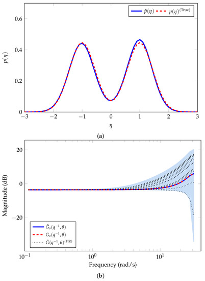
Figure 3.
Nominal model and error-model distribution estimated for Example 1. (a) Estimated error-model distribution. (b) Estimated nominal model .
On the other hand, we note that the SE method does not directly provide an uncertainty region. However, we compute M realizations of the model
with , where is the nominal model estimated and are obtained from M different realizations using the GMM in Equation (4) with the estimated parameters obtained by using our proposed SE method. In addition, we use the PEM [1,2] to estimate the system model with a high order FIR model. We consider the measurements of 25 independent experiments, and we estimate a 10th order FIR system model, , for each independent experiment in order to validate the uncertainty region estimated.
Figure 3b shows the magnitude of the frequency response corresponding to the average of all MC simulations for the estimated nominal model (blue line). The red-dashed line corresponds to the nominal system model in Equation (36), i.e., . The blue-shaded region represents the area of the corresponding uncertainty region estimated of the true system. We observe an accurate estimation of the nominal system model. We also observe that the FIR models estimated (black-dotted lines) lie in the uncertainty region obtained with our proposed method.
5.2. Example 2: A Resistor-Capacitor System Model with Non-Gaussian-Sum Uncertainties
Consider the system in Equation (2) as follows:
where is the sampled period, and is the time constant with , and is uniformly distributed as . We consider that the sampled period is known.
For the SE method, we consider an output-error nominal model with a FIR error-model as follows:
The distribution of the parameters of the error-model is modeled using a GMM with , components. The vector of parameter to be estimated is . As in the previous example, the uncertainty region is obtained from Equation (38) with , where is obtained from M different realizations using the GMM in Equation (4) with the estimated parameters . In addition, the initial values used for our proposed EM algorithm are given by , , , , , .
For comparison purposes, we estimate the system uncertainty and the nominal model using MEM approach [33]. The nominal model estimated, , corresponds to the average of all PEM estimations obtained using the original structure given in Equation (39), i.e., and , from the all independent experiments. In order to obtain the residuals, we compute for each independent experiment. The error-model, , is obtained from the residual data as follows:
where is a zero-mean Gaussian noise sequence which is assumed to be uncorrelated with the input signal . Thus, we consider a 10th order FIR system model for and we use the PEM [2] to estimate the error-model parameters for each experiment. The uncertainty region is computed by adding frequency by frequency the average of the all error-model estimated to the nominal model.
Finally, we consider the measurements of 25 independent experiments and we obtain an estimation of the system model in Equation (39), , using PEM with and for each independent experiment in order to validate the uncertainty region estimated for both SE and MEM approach.
Figure 4a shows the magnitude of the frequency response corresponding to the nominal model and the uncertainty region estimated using SE approach. The red-dashed line corresponds to the system model in Equation (39) considering the time constant without uncertainty, i.e., . The blue line corresponds to the average of all MC simulations for the estimated nominal model. We observe an accurate estimation for the nominal model with and noise variance . The blue-shaded area corresponds to the uncertainty region estimated for the true system. Similarly, Figure 4b shows the magnitude of the frequency response corresponding to the nominal model estimated (blue line) and the uncertainty region estimated (blue-shaded area) from the residuals using MEM. We also observe an accurate estimation of the nominal model with and noise variance . In addition, we observe in Figure 4a,b that PEM estimations, , lie in the uncertainty region obtained using both SE approach and MEM. However, SE method describes better the uncertainty region than MEM method, specifically, the error-model at low frequencies.
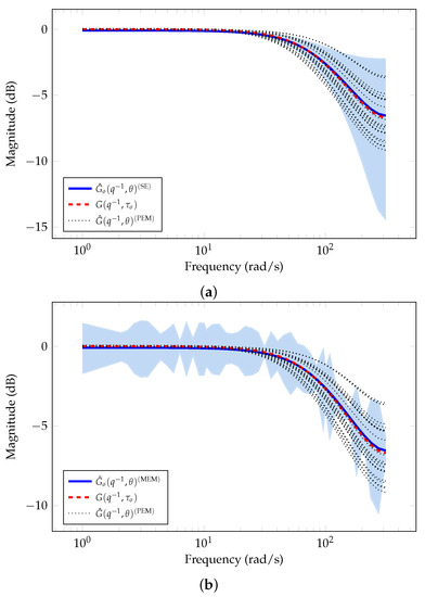
Figure 4.
Nominal model and uncertainty region estimated using SE and MEM for Example 2. (a) System model estimated with SE. (b) System model estimated with MEM.
6. Conclusions
In this paper, we have addressed the uncertainty modeling problem by combining the SE approach with GMMs. We proposed an identification algorithm using ML principle to estimate both the nominal model and the distribution of the parameters of the error-model as a GMM. An EM algorithm is proposed to solve the ML estimation problem providing closed-form expressions for the estimators of the GMM parameters and the noise variance. In the simulation examples, we considered two scenarios: (i) identification of a system model with a structure defined with SE approach using a nominal model and an error-model as a FIR system with Gaussian mixture distribution, and (ii) identification of a system model with non-Gaussian uncertainties in the parameters does not correspond to the SE framework. For both cases, we obtained accurate estimations of the nominal system model. Finally, our proposed method provided a good description of the uncertainty region in the system for the simulation examples.
Author Contributions
Conceptualization, R.O. and J.C.A.; formal analysis, R.O., R.C. and J.C.A.; funding acquisition, R.O., R.C. and J.C.A.; investigation, R.O., R.C., P.E. and J.C.A.; methodology, R.O. and J.C.A.; resources, J.C.A.; software, R.O.; validation, P.E.; visualization, P.E.; writing—original draft preparation, R.O., R.C., P.E. and J.C.A.; writing, review, and editing, R.O., R.C., P.E., J.C.A. All authors have read and agreed to the published version of the manuscript.
Funding
PIIC 05/2019 of DPP at Universidad Técnica Federico Santa María; ANID-FONDECYT 1211630 and 11201187; Advanced Center for Electrical and Electronic Engineering, AC3E, Basal Project FB0008, ANID, Chile.
Institutional Review Board Statement
Not applicable.
Informed Consent Statement
Not applicable.
Data Availability Statement
No new data were created or analyzed in this study. Data sharing is not applicable to this article.
Conflicts of Interest
The authors declare no conflict of interest.
Abbreviations
The following abbreviations are used in this manuscript:
| EM: | Expectation-Maximization |
| FIR: | Finite impulse response |
| GMM: | Gaussian mixture model |
| MC: | Monte Carlo |
| MEM: | Model error modeling |
| ML: | Maximum likelihood |
| PDF: | Probability density function |
| PEM: | Prediction error method |
| SE: | Stochastic embedding |
Appendix A. Maximum Likelihood Formulation with SE Approach
Let us consider that is a collection of measurements for each experiment . Then, the likelihood function, , for the system model in Equation (13) using the GMM in Equation (4) can be obtained by marginalizing the hidden variable, , as follows:
where
with , . The log-likelihood function, , is then given by
Consider the following identities:
Appendix B. Computing the Complete Likelihood Function
From the likelihood function in Equation (16), we have:
where and are given by Equations (A9) and (A10), respectively. Let consider
where is a discrete random variable (hidden variable) such that is an indicator that determines if the rth observation arises from the ith component of the GMM in Equation (A3), that is,
Defining the complete data set as and utilizing the Bayes’ rule, the complete likelihood function is obtained as follows:
The complete log-likelihood function is given by:
Appendix C. EM Algorithm with GMMs Formulation
Appendix C.1. Computing the Auxiliary Function
Appendix C.2. Optimizing the Auxiliary Function
From Equation (A8), we have the following:
Let consider the following identity for a random variable x:
where , and .
Substituting Equations (A26) and (A28) in Equation (A22), and taking the derivative of Equation (A22) with respect to and equating to zero, yields:
Then, taking the derivative of Equation (A22) with respect to and equating to zero:
Then, taking the derivative of Equation (A22) with respect to and equating to zero yields:
For the parameter , we define as follows:
subject to . Then, using a Lagrange multiplier to deal with the constraint on , we define:
References
- Söderström, T.; Stoica, P. System Identification; Prentice-Hall, Inc.: Upper Saddle River, NJ, USA, 1988. [Google Scholar]
- Ljung, L. System Identification: Theory for the User; Prentice Hall PTR: Upper Saddle River, NJ, USA, 1999. [Google Scholar]
- Goodwin, G.C.; Payne, R.L. Dynamic System Identification: Experiment Design and Data Analysis; Academic Press: New York, NY, USA, 1977. [Google Scholar]
- Ljung, L.; Goodwin, G.C.; Agüero, J.C. Stochastic Embedding revisited: A modern interpretation. In Proceedings of the 53rd IEEE Conference on Decision and Control, Los Angeles, CA, USA, 15–17 December 2014; pp. 3340–3345. [Google Scholar]
- Jategaonkar, R.V. Flight Vehicle System Identification: A Time Domain Methodology, 2nd ed.; Progress in Astronautics and Aeronautics; v. 245; American Institute of Aeronautics and Astronautics, Inc.: Reston, VA, USA, 2006. [Google Scholar]
- Han, Z.; Li, W.; Shah, S.L. Robust Fault Diagnosis in the Presence of Process Uncertainties. IFAC Proc. Vol. 2002, 35, 473–478. [Google Scholar] [CrossRef]
- Nikoukhah, R.; Campbell, S. A Multi-Model Approach to Failure Detection in Uncertain Sampled-Data Systems. Eur. J. Control 2005, 11, 255–265. [Google Scholar] [CrossRef]
- Patton, R.J.; Frank, P.M.; Clark, R.N. Issues of Fault Diagnosis for Dynamic Systems, 1st ed.; Springer Publishing Company, Inc.: Berlin/Heidelberg, Germany, 2010. [Google Scholar]
- Escobet, T.; Bregon, A.; Pulido, B.; Puig, V. Fault Diagnosis of Dynamic Systems; Springer: Cham, Switzerland, 2019. [Google Scholar]
- Hamel, P.G.; Jategaonkar, R.V. Evolution of flight vehicle system identification. J. Aircr. 1996, 33, 9–28. [Google Scholar] [CrossRef]
- Jategaonkar, R.; Thielecke, F. Aircraft parameter estimation—A tool for development of aerodynamic databases. Sadhana 2006, 25, 119–135. [Google Scholar] [CrossRef]
- Rosić, B.V.; Diekmann, J.H. Methods for the Uncertainty Quantification of Aircraft Simulation Models. J. Aircr. 2015, 52, 1247–1255. [Google Scholar] [CrossRef]
- Mu, H.Q.; Liu, H.T.; Shen, J.H. Copula-Based Uncertainty Quantification (Copula-UQ) for Multi-Sensor Data in Structural Health Monitoring. Sensors 2020, 20, 5692. [Google Scholar] [CrossRef]
- Hilton, S.; Cairola, F.; Gardi, A.; Sabatini, R.; Pongsakornsathien, N.; Ezer, N. Uncertainty Quantification for Space Situational Awareness and Traffic Management. Sensors 2019, 19, 4361. [Google Scholar] [CrossRef]
- Guo, J.; Zhao, Y. Recursive projection algorithm on FIR system identification with binary-valued observations. Automatica 2013, 49, 3396–3401. [Google Scholar] [CrossRef]
- Moschitta, A.; Schoukens, J.; Carbone, P. Parametric System Identification Using Quantized Data. IEEE Trans. Instrum. Meas. 2015, 64, 2312–2322. [Google Scholar] [CrossRef]
- Cedeño, A.L.; Orellana, R.; Carvajal, R.; Agüero, J.C. EM-based identification of static errors-in-variables systems utilizing Gaussian Mixture models. IFAC-PapersOnLine 2020, 53, 863–868. [Google Scholar] [CrossRef]
- Orellana, R.; Escárate, P.; Curé, M.; Christen, A.; Carvajal, R.; Agüero, J.C. A method to deconvolve stellar rotational velocities-III. The probability distribution function via maximum likelihood utilizing finite distribution mixtures. Astron. Astrophys. 2019, 623, A138. [Google Scholar] [CrossRef]
- Agüero, J.C.; Goodwin, G.C.; Yuz, J.I. System identification using quantized data. In Proceedings of the 46th IEEE Conference on Decision and Control, New Orleans, LA, USA, 12–14 December 2007; pp. 4263–4268. [Google Scholar]
- Godoy, B.I.; Goodwin, G.C.; Agüero, J.C.; Marelli, D.; Wigren, T. On identification of FIR systems having quantized output data. Automatica 2011, 47, 1905–1915. [Google Scholar] [CrossRef]
- Godoy, B.I.; Agüero, J.C.; Carvajal, R.; Goodwin, G.C.; Yuz, J.I. Identification of sparse FIR systems using a general quantisation scheme. Int. J. Control 2014, 87, 874–886. [Google Scholar] [CrossRef]
- Agüero, J.C.; González, K.; Carvajal, R. EM-based identification of ARX systems having quantized output data. IFAC-PapersOnLine 2017, 50, 8367–8372. [Google Scholar] [CrossRef]
- Carvajal, R.; Godoy, B.I.; Agüero, J.C.; Goodwin, G.C. EM-based sparse channel estimation in OFDM systems. In Proceedings of the IEEE 13th International Workshop on Signal Processing Advances in Wireless Communications, Çeşme, Turkey, 17–20 June 2012; pp. 530–534. [Google Scholar]
- Carvajal, R.; Aguero, J.C.; Godoy, B.I.; Goodwin, G.C. EM-Based Maximum-Likelihood Channel Estimation in Multicarrier Systems With Phase Distortion. IEEE Trans. Veh. Technol. 2013, 62, 152–160. [Google Scholar] [CrossRef]
- Carnduff, S. Flight Vehicle System Identification: A Time-Domain Methodology. Aeronaut. J. 2015, 119, 930–931. [Google Scholar] [CrossRef]
- Goodwin, G.C.; Salgado, M.E. A stochastic embedding approach for quantifying uncertainty in the estimation of restricted complexity models. Int. J. Adapt. Control Signal Process. 1989, 3, 333–356. [Google Scholar] [CrossRef]
- Van den Hof, P.; Wahlberg, B.; Heuberger, P.; Ninness, B.; Bokor, J.; Oliveira e Silva, T. Modelling and Identification with Rational Orthogonal Basis Functions. IFAC Proc. Vol. 2000, 33, 445–455. [Google Scholar] [CrossRef]
- Peralta, P.; Ruiz, R.O.; Taflanidis, A.A. Bayesian identification of electromechanical properties in piezoelectric energy harvesters. Mech. Syst. Signal Process. 2020, 141, 106506. [Google Scholar] [CrossRef]
- Goodwin, G.; Graebe, S.; Salgado, M.E. Control Systems Design; Prentice Hall: Upper Saddle River, NJ, USA, 2001. [Google Scholar]
- Douma, S.G.; Van den Hof, P.M. Relations between uncertainty structures in identification for robust control. Automatica 2005, 41, 439–457. [Google Scholar] [CrossRef]
- Calafiore, G.C.; Campi, M.C. The scenario approach to robust control design. IEEE Trans. Autom. Control 2006, 51, 742–753. [Google Scholar] [CrossRef]
- Milanese, M.; Vicino, A. Optimal estimation theory for dynamic systems with set membership uncertainty: An overview. Automatica 1991, 27, 997–1009. [Google Scholar] [CrossRef]
- Ljung, L. Model Error Modeling and Control Design. IFAC Proc. Vol. 2000, 33, 31–36. [Google Scholar] [CrossRef]
- Goodwin, G.C.; Gevers, M.; Ninness, B. Quantifying the error in estimated transfer functions with application to model order selection. IEEE Trans. Autom. Control 1992, 37, 913–928. [Google Scholar] [CrossRef]
- Delgado, R.A.; Goodwin, G.C.; Carvajal, R.; Agüero, J.C. A novel approach to model error modelling using the expectation-maximization algorithm. In Proceedings of the 51st IEEE Conference on Decision and Control, Maui, HI, USA, 10–13 December 2012; pp. 7327–7332. [Google Scholar]
- Dempster, A.; Laird, N.; Rubin, D. Maximum likelihood from incomplete data via the EM algorithm. J. R. Stat. Soc. Ser. B 1977, 39, 1–38. [Google Scholar]
- Ljung, L.; Goodwin, G.C.; Agüero, J.C.; Chen, T. Model Error Modeling and Stochastic Embedding. IFAC-PapersOnLine 2015, 48, 75–79. [Google Scholar] [CrossRef]
- Pillonetto, G.; Nicolao, G.D. A new kernel-based approach for linear system identification. Automatica 2010, 46, 81–93. [Google Scholar] [CrossRef]
- Ljung, L.; Chen, T.; Mu, B. A shift in paradigm for system identification. Int. J. Control 2020, 93, 173–180. [Google Scholar] [CrossRef]
- Anderson, B.; Moore, J. Optimal Filtering; Prentice-Hall: Englewood Cliffs, NJ, USA, 1979. [Google Scholar]
- Söderström, T. Discrete-Time Stochastic Systems: Estimation and Control, 2nd ed.; Springer: Berlin/Heidelberg, Germany, 2002. [Google Scholar]
- Balenzuela, M.P.; Dahlin, J.; Bartlett, N.; Wills, A.G.; Renton, C.; Ninness, B. Accurate Gaussian Mixture Model Smoothing using a Two-Filter Approach. In Proceedings of the IEEE Conference on Decision and Control, Miami, FL, USA, 17–19 December 2018; pp. 694–699. [Google Scholar]
- Bittner, G.; Orellana, R.; Carvajal, R.; Agüero, J.C. Maximum Likelihood identification for Linear Dynamic Systems with finite Gaussian mixture noise distribution. In Proceedings of the IEEE CHILEAN Conference on Electrical, Electronics Engineering, Information and Communication Technologies (CHILECON), Valparaíso, Chile, 13–27 November 2019; pp. 1–7. [Google Scholar]
- Orellana, R.; Bittner, G.; Carvajal, R.; Agüero, J.C. Maximum Likelihood estimation for non-minimum-phase noise transfer function with Gaussian mixture noise distribution. Automatica 2021. under review. [Google Scholar]
- Sorenson, H.W.; Alspach, D.L. Recursive Bayesian estimation using Gaussian sums. Automatica 1971, 7, 465–479. [Google Scholar] [CrossRef]
- Dahlin, J.; Wills, A.; Ninness, B. Sparse Bayesian ARX models with flexible noise distributions. IFAC-PapersOnLine 2018, 51, 25–30. [Google Scholar] [CrossRef]
- Orellana, R.; Carvajal, R.; Agüero, J.C. Empirical Bayes estimation utilizing finite Gaussian Mixture Models. In Proceedings of the IEEE CHILEAN Conference on Electrical, Electronics Engineering, Information and Communication Technologies (CHILECON), Valparaíso, Chile, 13–27 November 2019; pp. 1–6. [Google Scholar]
- Orellana, R.; Carvajal, R.; Agüero, J.C.; Goodwin, G.C. Model Error Modelling using a Stochastic Embedding approach with Gaussian Mixture Models for FIR system. IFAC-PapersOnLine 2020, 53, 845–850. [Google Scholar] [CrossRef]
- Carvajal, R.; Orellana, R.; Katselis, D.; Escárate, P.; Agüero, J.C. A data augmentation approach for a class of statistical inference problems. PLoS ONE 2018, 13, e0208499. [Google Scholar] [CrossRef]
- Lo, J. Finite-dimensional sensor orbits and optimal nonlinear filtering. IEEE Trans. Inf. Theory 1972, 18, 583–588. [Google Scholar] [CrossRef]
- Yu, C.; Verhaegen, M. Data-driven fault estimation of non-minimum phase LTI systems. Automatica 2018, 92, 181–187. [Google Scholar] [CrossRef]
- Campi, M.C. The problem of pole-zero cancellation in transfer function identification and application to adaptive stabilization. Automatica 1996, 32, 849–857. [Google Scholar] [CrossRef]
- Heuberger, P.; Van den Hof, P.; Bosgra, O. A Generalized Orthonormal Basis for Linear Dynamical Systems. IEEE Trans. Autom. Control 1995, 40, 451–465. [Google Scholar] [CrossRef]
- Chen, T.; Ljung, L. Implementation of algorithms for tuning parameters in regularized least squares problems in system identification. Automatica 2013, 49, 2213–2220. [Google Scholar] [CrossRef]
- Jin, C.; Zhang, Y.; Balakrishnan, S.; Wainwright, M.; Jordan, M. Local Maxima in the Likelihood of Gaussian Mixture Models: Structural Results and Algorithmic Consequences. In Proceedings of the 29th Conference on Neural Information Processing Systems, Barcelona, Spain, 5–10 December 2016; pp. 4123–4131. [Google Scholar]
- McLachlan, G.J.; Peel, D. Finite Mixture Models; John Wiley & Sons: New York, NY, USA, 2000. [Google Scholar]
- Frühwirth-Schnatter, S.; Celeux, G.; Robert, C. Handbook of Mixture Analysis; Chapman and Hall/CRC: New York, NY, USA, 2018. [Google Scholar]
- Gibson, S.; Ninness, B. Robust maximum-likelihood estimation of multivariable dynamic systems. Automatica 2005, 41, 1667–1682. [Google Scholar] [CrossRef]
- Gopaluni, R.B. A particle filter approach to identification of nonlinear processes under missing observations. Can. J. Chem. Eng. 2008, 86, 1081–1092. [Google Scholar] [CrossRef]
- Agüero, J.C.; Tang, W.; Yuz, J.I.; Delgado, R.; Goodwin, G.C. Dual time–frequency domain system identification. Automatica 2012, 48, 3031–3041. [Google Scholar] [CrossRef]
- Wright, S. Coordinate descent algorithms. Math. Program. 2015, 151, 3–34. [Google Scholar] [CrossRef]
- Lichota, P. Inclusion of the D-optimality in multisine manoeuvre design for aircraft parameter estimation. J. Theor. Appl. Mech. 2016, 54, 87–98. [Google Scholar] [CrossRef]
- Pawełek, A.; Lichota, P. Arrival air traffic separations assessment using Maximum Likelihood Estimation and Fisher Information Matrix. In Proceedings of the 20th International Carpathian Control Conference, Krakow-Wieliczka, Poland, 26–29 May 2019; pp. 1–6. [Google Scholar]


Publisher’s Note: MDPI stays neutral with regard to jurisdictional claims in published maps and institutional affiliations. |
© 2021 by the authors. Licensee MDPI, Basel, Switzerland. This article is an open access article distributed under the terms and conditions of the Creative Commons Attribution (CC BY) license (https://creativecommons.org/licenses/by/4.0/).