
Uniaxial 3D Measurement with Auto-Synchronous Phase-Shifting and Defocusing Based on a Tilted Grating


Abstract
1. Introduction
2. Principle
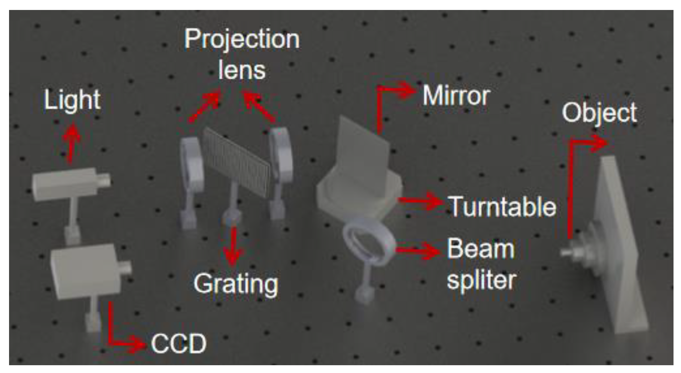
2.1. The Structure of the Proposed Measurement System
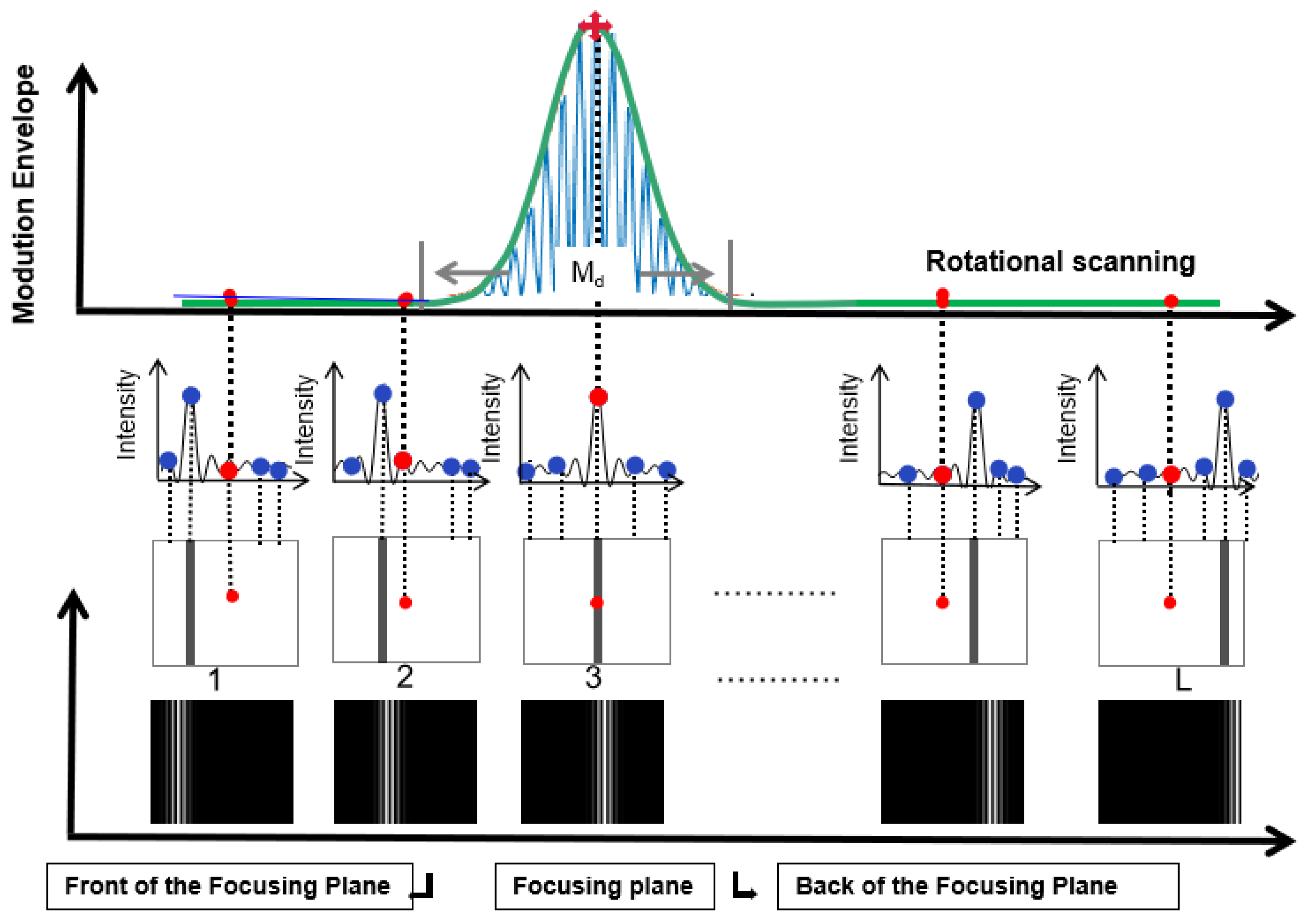
2.2. The Measuring Principle of the Proposed Measurement System
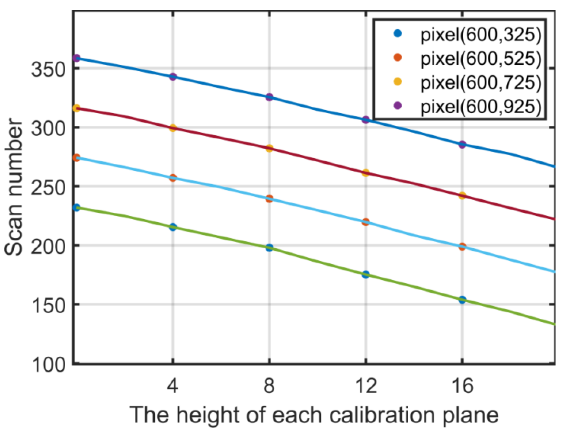
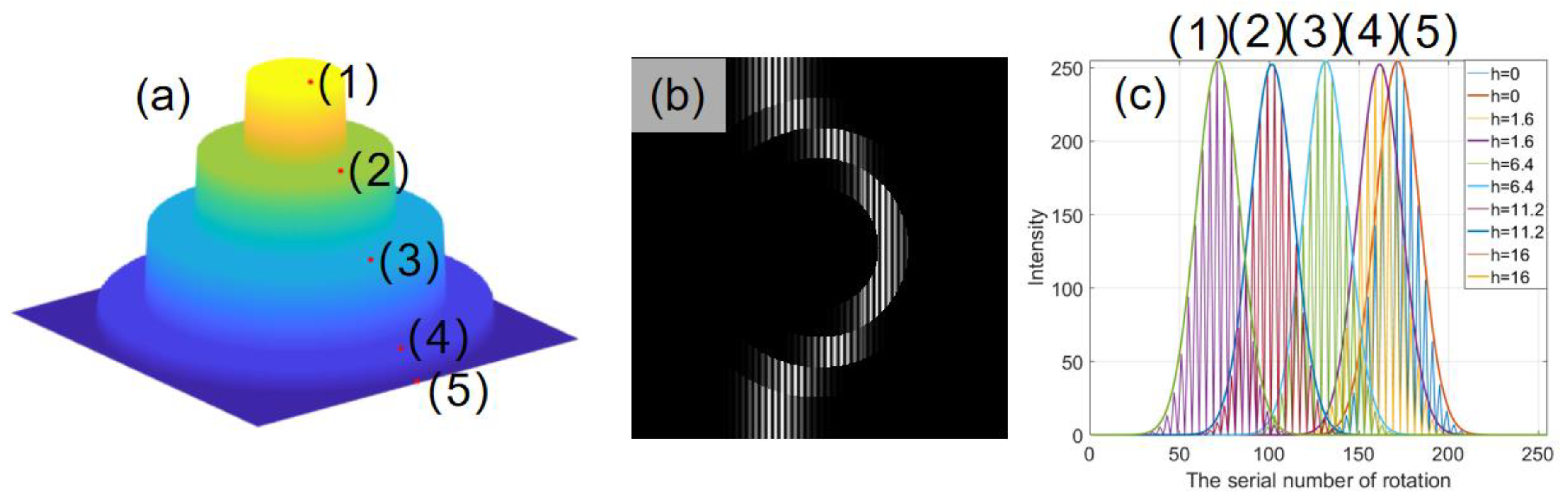
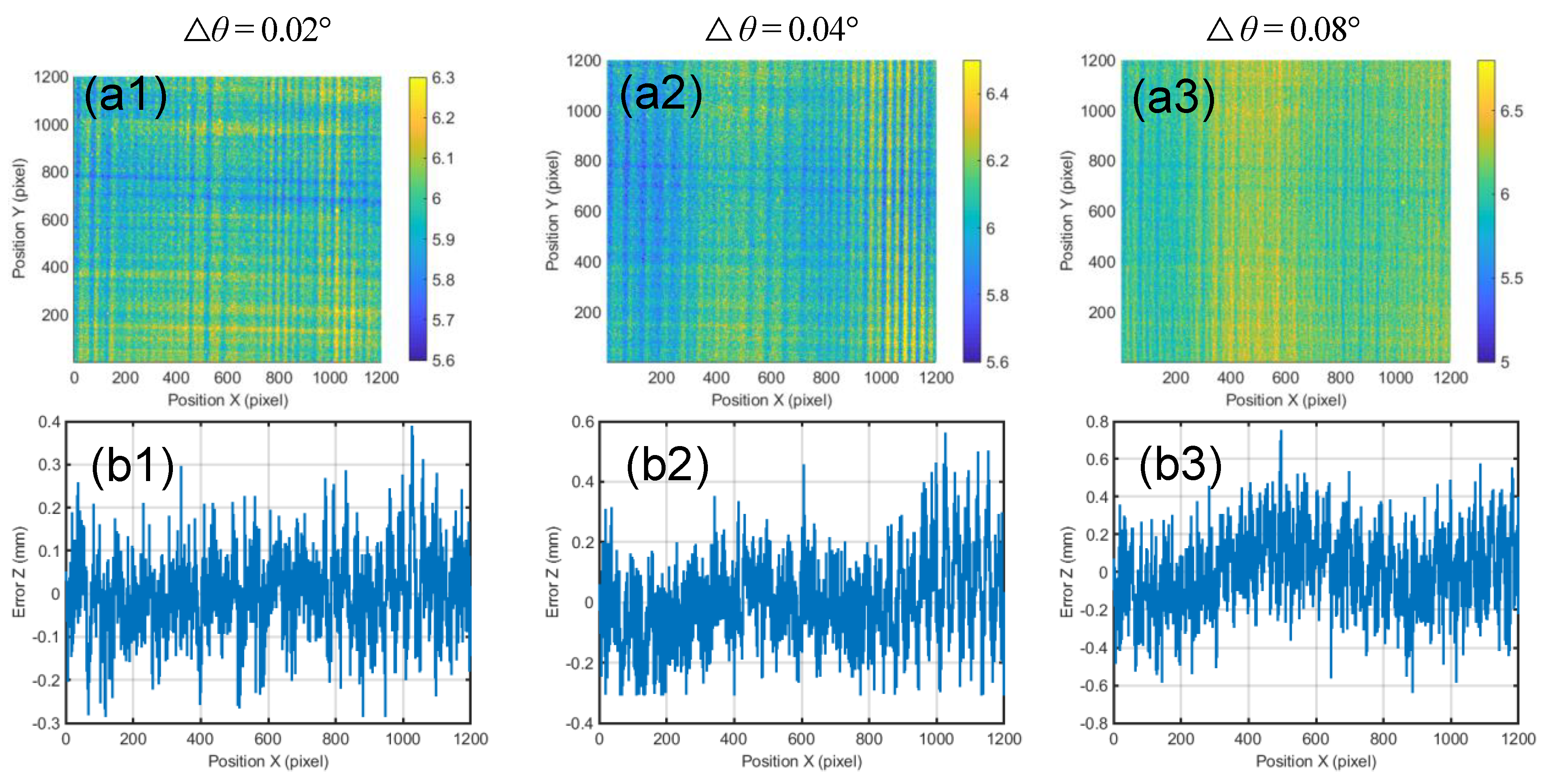
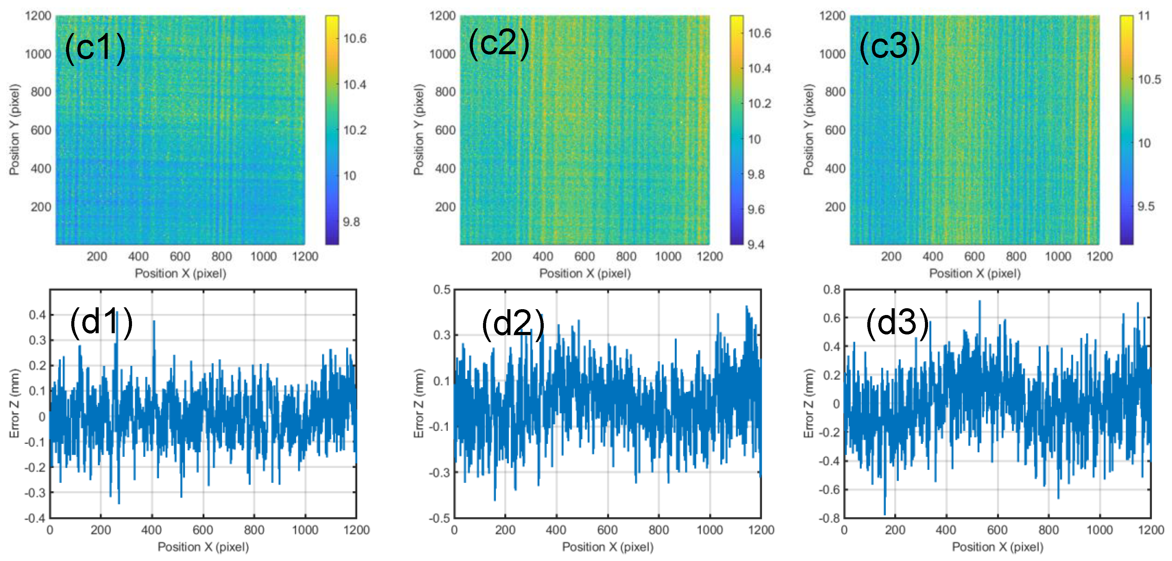
3. Simulation
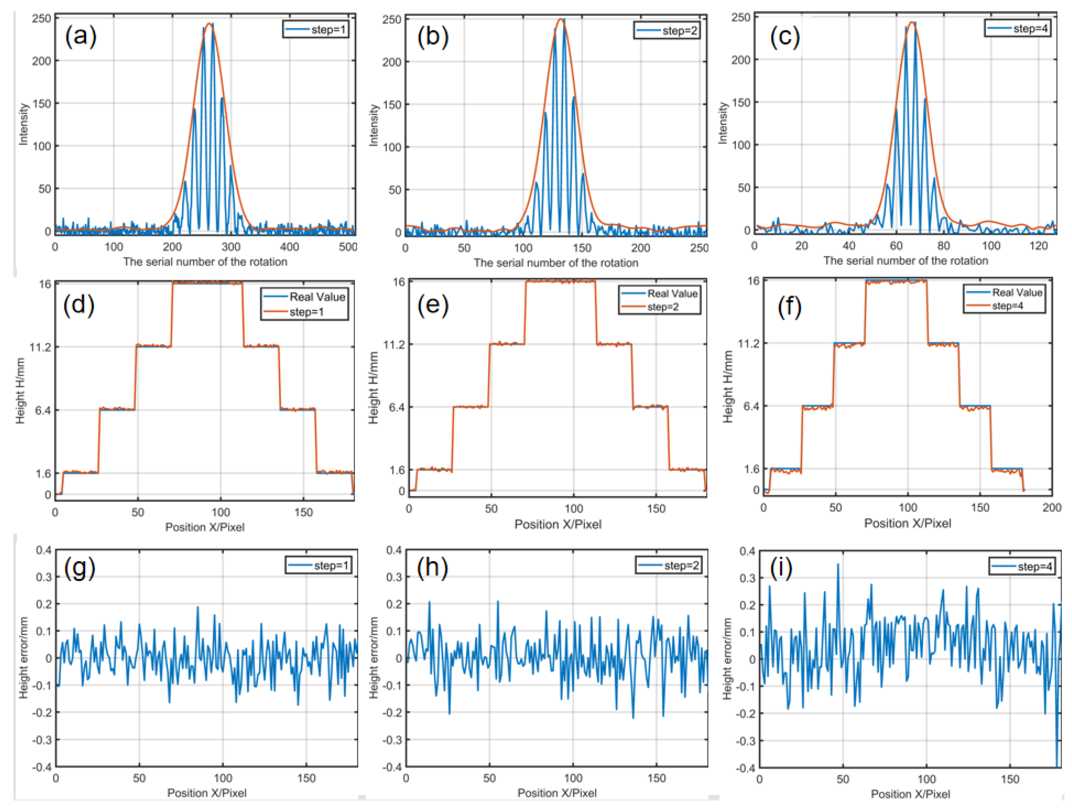
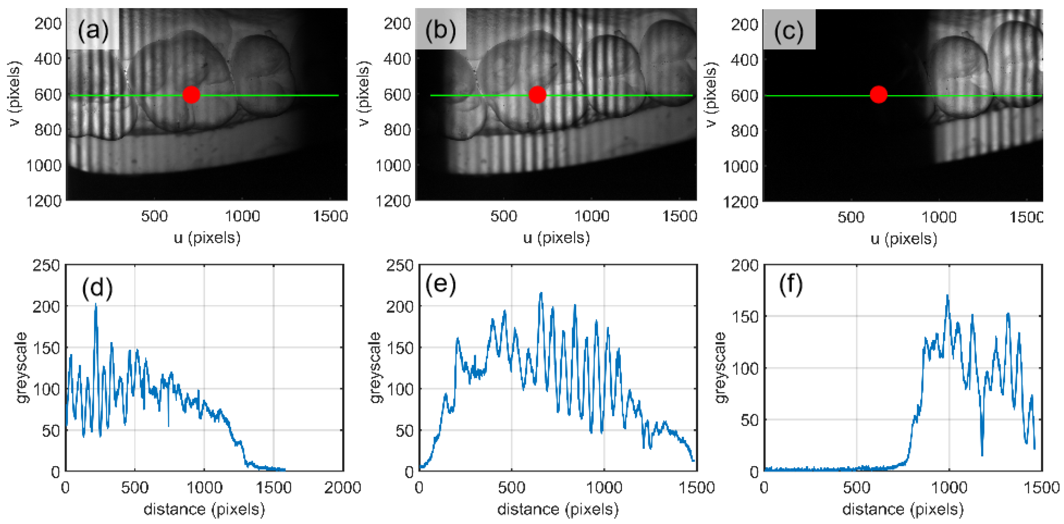
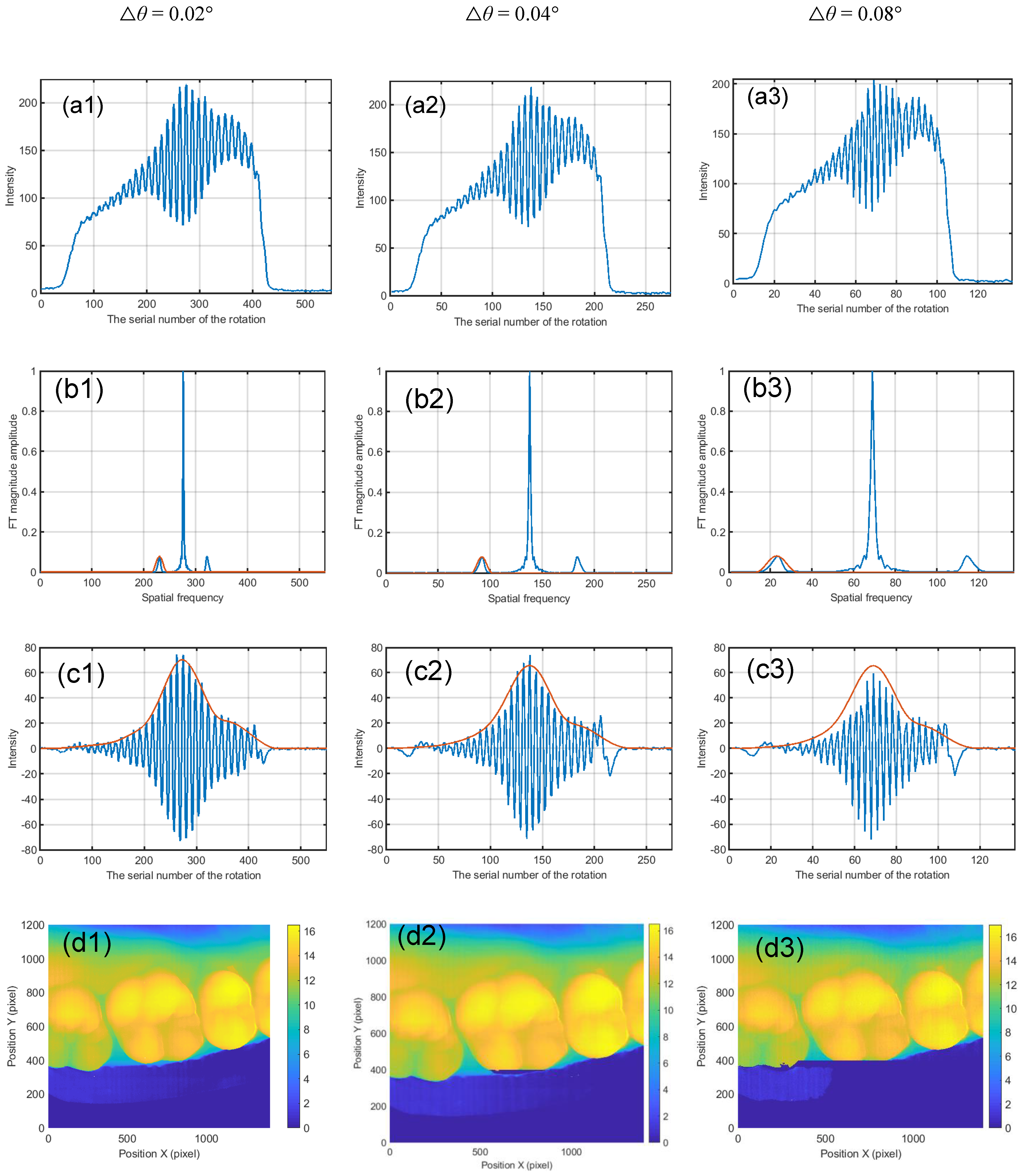
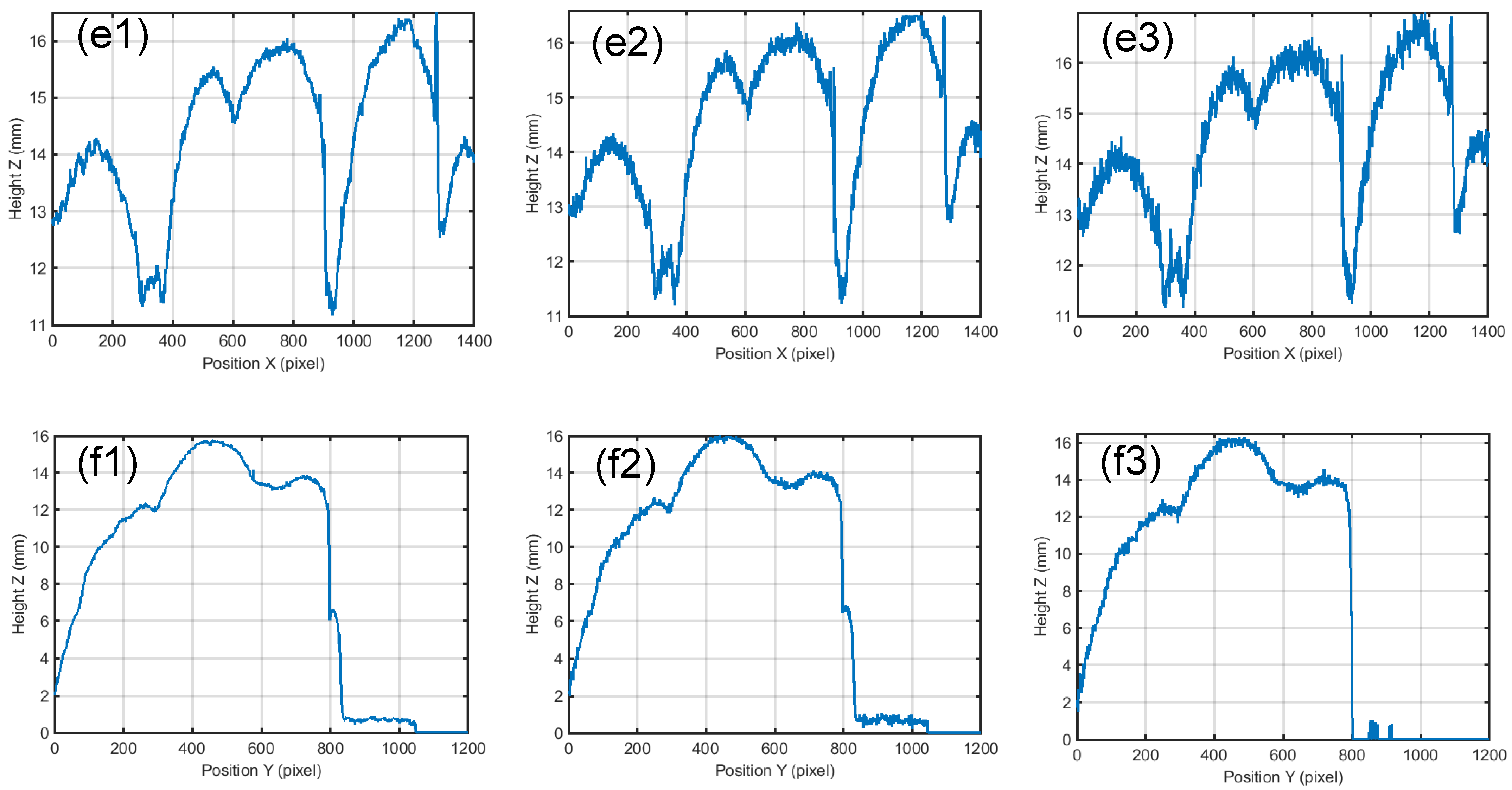
4. Experiment
5. Conclusions and Discussion
Author Contributions
Funding
Institutional Review Board Statement
Informed Consent Statement
Conflicts of Interest
References
- Su, X.; Su, L.; Li, W.; Xiang, L. New 3D profilometry based on modulation measurement. Proc. SPIE Int. Soc. Opt. Eng. 1999, 19, 1–7. [Google Scholar]
- Zheng, Y.; Wang, Y.; Li, B. Active shape from projection defocus profilometry. Opt. Lasers Eng. 2020, 134, 106277. [Google Scholar] [CrossRef]
- Zheng, Y.; Kessel, A.; Häusler, G. Better 3D inspection with structured illumination: Signal formation and precision. Appl. Opt. 2015, 54, 6652–6660. [Google Scholar]
- Ying, X.; Ekstrand, L.; Song, Z. Uniaxial 3D Shape Measurement with Projector Defocusing. Proc. SPIE 2011, 8133. [Google Scholar] [CrossRef]
- Su, L.; Su, X.; Li, W.; Xiang, L. Application of modulation measurement profilometry to objects with surface holes. Appl. Opt. 1999, 38, 1153–1158. [Google Scholar] [CrossRef] [PubMed]
- Yang, Z.; Bielke, A.; HäUsler, G. Better three-dimensional inspection with structured illumination: Speed. Appl. Opt. 2016, 55, 1713. [Google Scholar] [CrossRef] [PubMed]
- Mizutani, Y.; Kuwano, R.; Otani, Y.; Umeda, N.; Yoshizawa, T. Three-dimensional shape measurement using focus method by using liquid crystal grating and liquid varifocus lens. Proc. SPIE Int. Soc. Opt. Eng. 2005, 6000, 336–431. [Google Scholar]
- Jing, H.; Su, X.; You, Z.; Lu, M. Uniaxial 3D shape measurement using DMD grating and EF lens. Optik 2017, 138, 487–493. [Google Scholar] [CrossRef]
- Zhong, M.; Cui, J.; Hyun, J.; Pan, L.; Duan, P.; Zhang, S. Uniaxial three-dimensional phase-shifting profilometry using a dual-telecentric structured light system in micro-scale devices. Meas. Sci. Technol. 2020, 31, 085003. [Google Scholar] [CrossRef]
- Dou, Y.; Su, X.; Chen, Y.; Ying, W. A flexible fast 3D profilometry based on modulation measurement. Opt. Lasers Eng. 2011, 49, 376–383. [Google Scholar] [CrossRef]
- Takeda, M.; Ina, H.; Kobayashi, S. Fourier-transform method of fringe-pattern analysis for computer-based topography and interferometry. Rev. Sci. Instrum. 1982, 72, 156–160. [Google Scholar] [CrossRef]
- Lu, M.; Su, X.; Cao, Y.; You, Z.; Zhong, M. Modulation measuring profilometry with cross grating projection and single shot for dynamic 3D shape measurement. Opt. Lasers Eng. 2016, 87, 103–110. [Google Scholar] [CrossRef]
- Liu, Y.; Zhang, Q.; Su, X. 3D shape from phase errors by using binary fringe with multi-step phase-shift technique. Opt. Lasers Eng. 2015, 74, 22–27. [Google Scholar] [CrossRef]
- Zhong, M.; Su, X.; Chen, W.; You, Z.; Lu, M.; Jing, H. Modulation measuring profilometry with auto-synchronous phase shifting and vertical scanning. Opt. Express 2014, 22, 31620. [Google Scholar] [CrossRef] [PubMed]
- Wang, Y.; Zhang, L. High-accuracy dithering-based three-dimensional data compression algorithms by phase correction. Appl. Opt. 2016, 55, 58. [Google Scholar] [CrossRef] [PubMed]
- Takeda, M. Spatial-carrier fringe-pattern analysis and its applications to precision interferometry and profilometry: An overview. Ind. Metrol. 1990, 1, 79–99. [Google Scholar] [CrossRef]
- Shao, S.; Su, X.; Zhang, Q.; Wang, H. Application of modulation measurement profilometry in the measurement of complex surface shapes. Acta Opt. 2004, 24, 1623–1628. [Google Scholar]


| Rotation Interval △θ | Height = 6 mm | Height = 10 mm | ||
|---|---|---|---|---|
| Mean | RMS | Mean | RMS | |
| 0.02° | 5.9016 | 0.1169 | 10.1104 | 0.1157 |
| 0.04° | 5.9464 | 0.1607 | 10.0481 | 0.1507 |
| 0.08° | 5.9545 | 0.2261 | 10.0258 | 0.2328 |
Publisher’s Note: MDPI stays neutral with regard to jurisdictional claims in published maps and institutional affiliations. |
© 2021 by the authors. Licensee MDPI, Basel, Switzerland. This article is an open access article distributed under the terms and conditions of the Creative Commons Attribution (CC BY) license (https://creativecommons.org/licenses/by/4.0/).
Share and Cite
Ren, H.; Liu, Y.; Wang, Y.; Liu, N.; Yu, X.; Su, X. Uniaxial 3D Measurement with Auto-Synchronous Phase-Shifting and Defocusing Based on a Tilted Grating. Sensors 2021, 21, 3730. https://doi.org/10.3390/s21113730
Ren H, Liu Y, Wang Y, Liu N, Yu X, Su X. Uniaxial 3D Measurement with Auto-Synchronous Phase-Shifting and Defocusing Based on a Tilted Grating. Sensors. 2021; 21(11):3730. https://doi.org/10.3390/s21113730
Chicago/Turabian StyleRen, Hui, Yuankun Liu, Yajun Wang, Ningyi Liu, Xin Yu, and Xianyu Su. 2021. "Uniaxial 3D Measurement with Auto-Synchronous Phase-Shifting and Defocusing Based on a Tilted Grating" Sensors 21, no. 11: 3730. https://doi.org/10.3390/s21113730
APA StyleRen, H., Liu, Y., Wang, Y., Liu, N., Yu, X., & Su, X. (2021). Uniaxial 3D Measurement with Auto-Synchronous Phase-Shifting and Defocusing Based on a Tilted Grating. Sensors, 21(11), 3730. https://doi.org/10.3390/s21113730