
LiDAR Point Cloud Generation for SLAM Algorithm Evaluation


Abstract
1. Introduction
2. Background
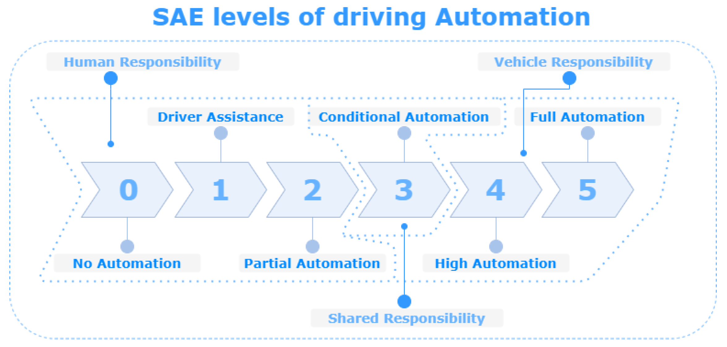
2.1. Autonomy
2.2. Equipment of Autonomous Vehicles
2.3. Accuracy of Sensors
2.4. Components of Autonomous Driving System
2.5. 3D SLAM Algorithms
2.6. Testing of Autonomous Vehicles
3. Related Work
4. Methodology
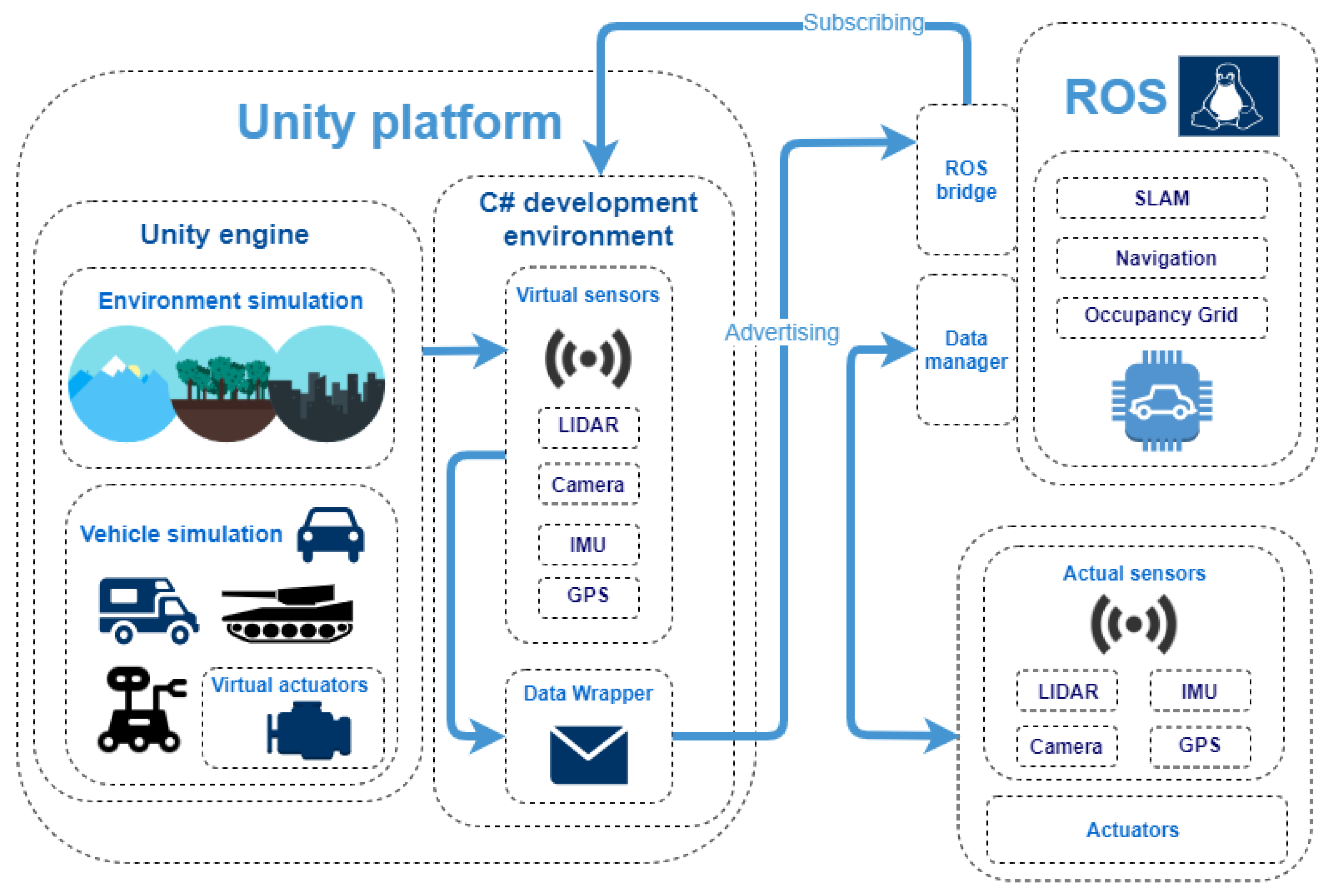
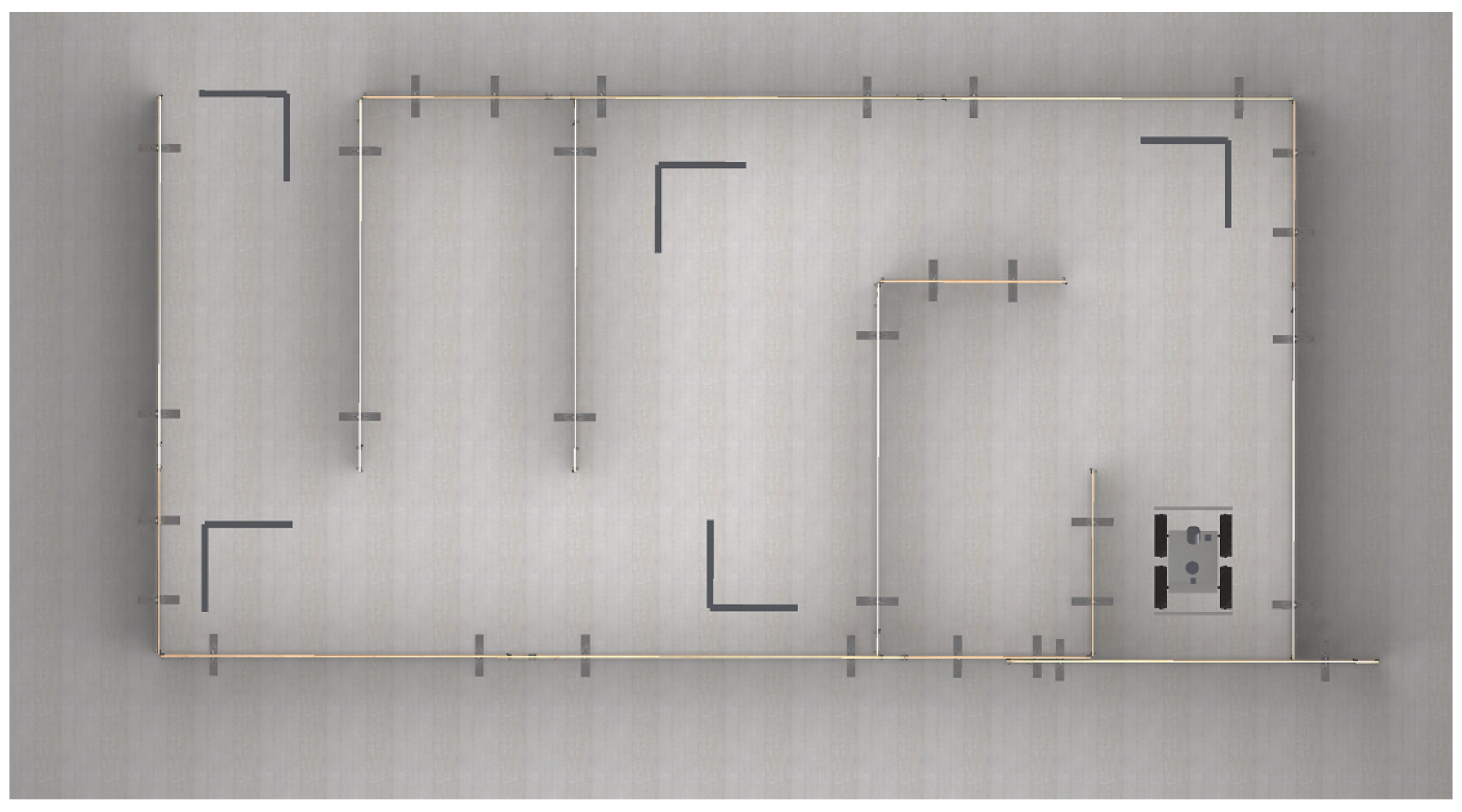
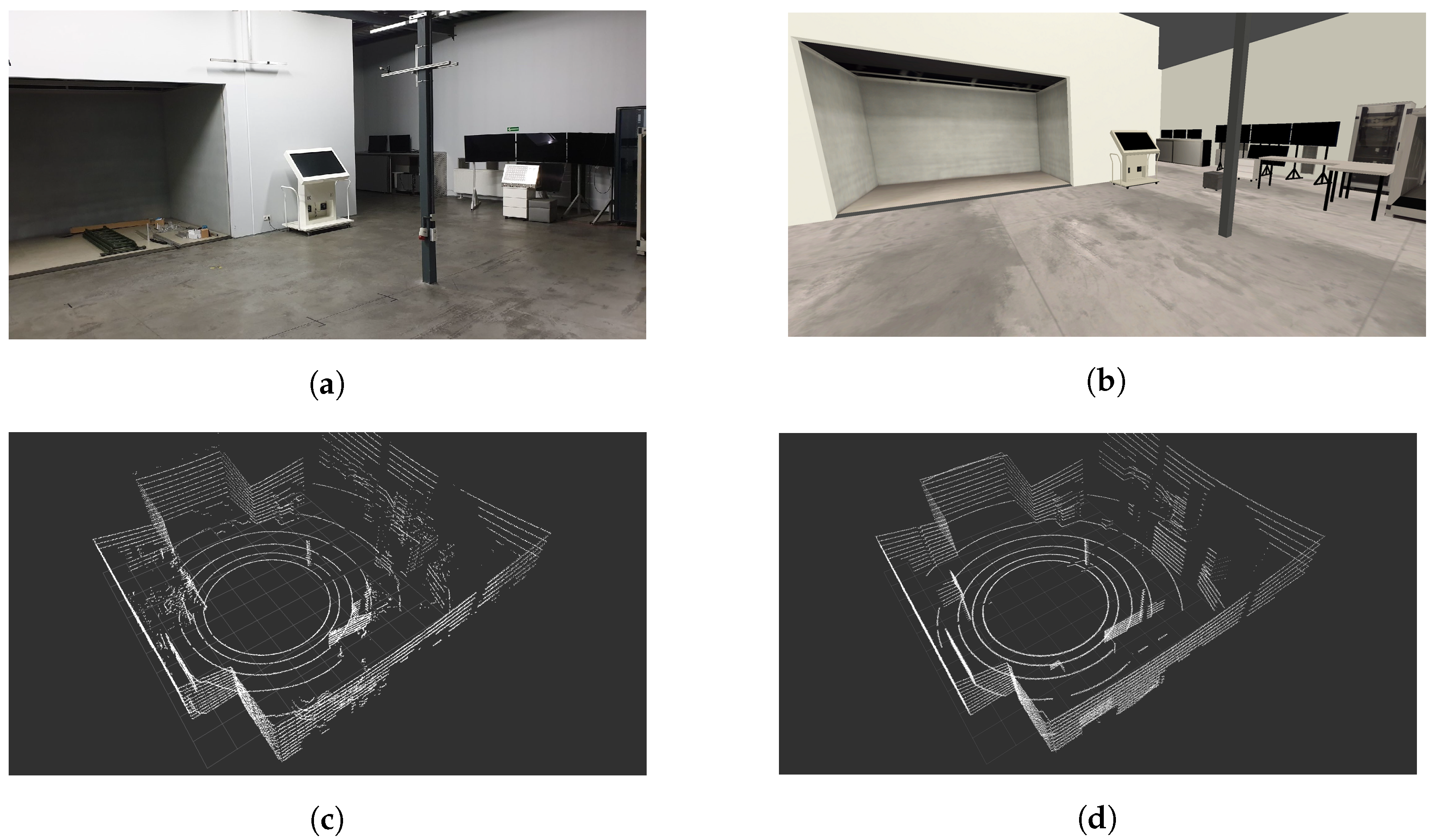
4.1. Experimental Setup
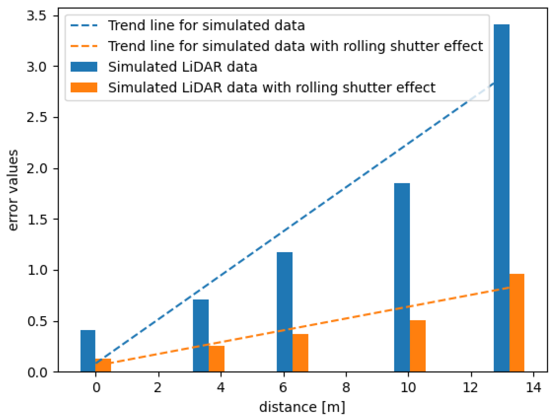
4.2. Simulation of the Rolling Shutter Effect
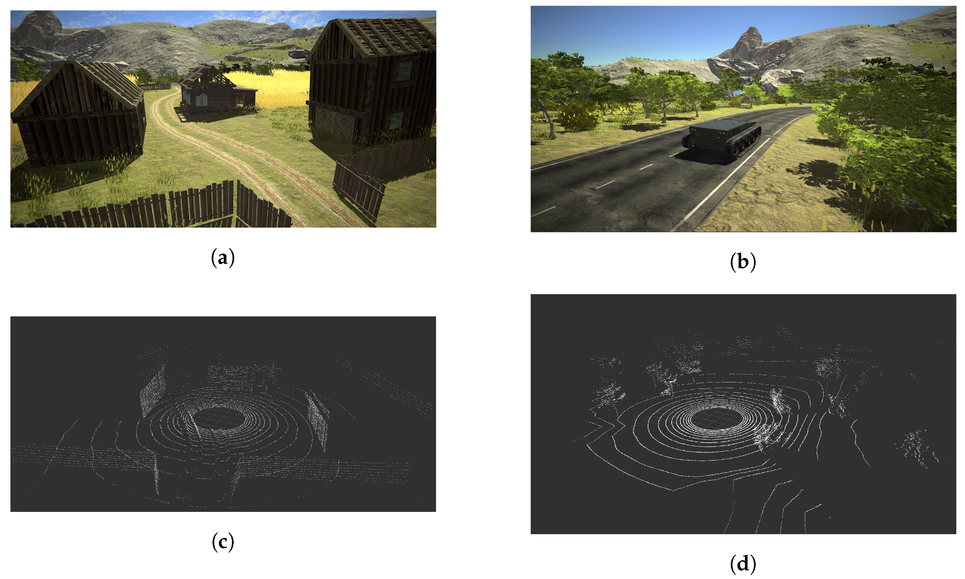
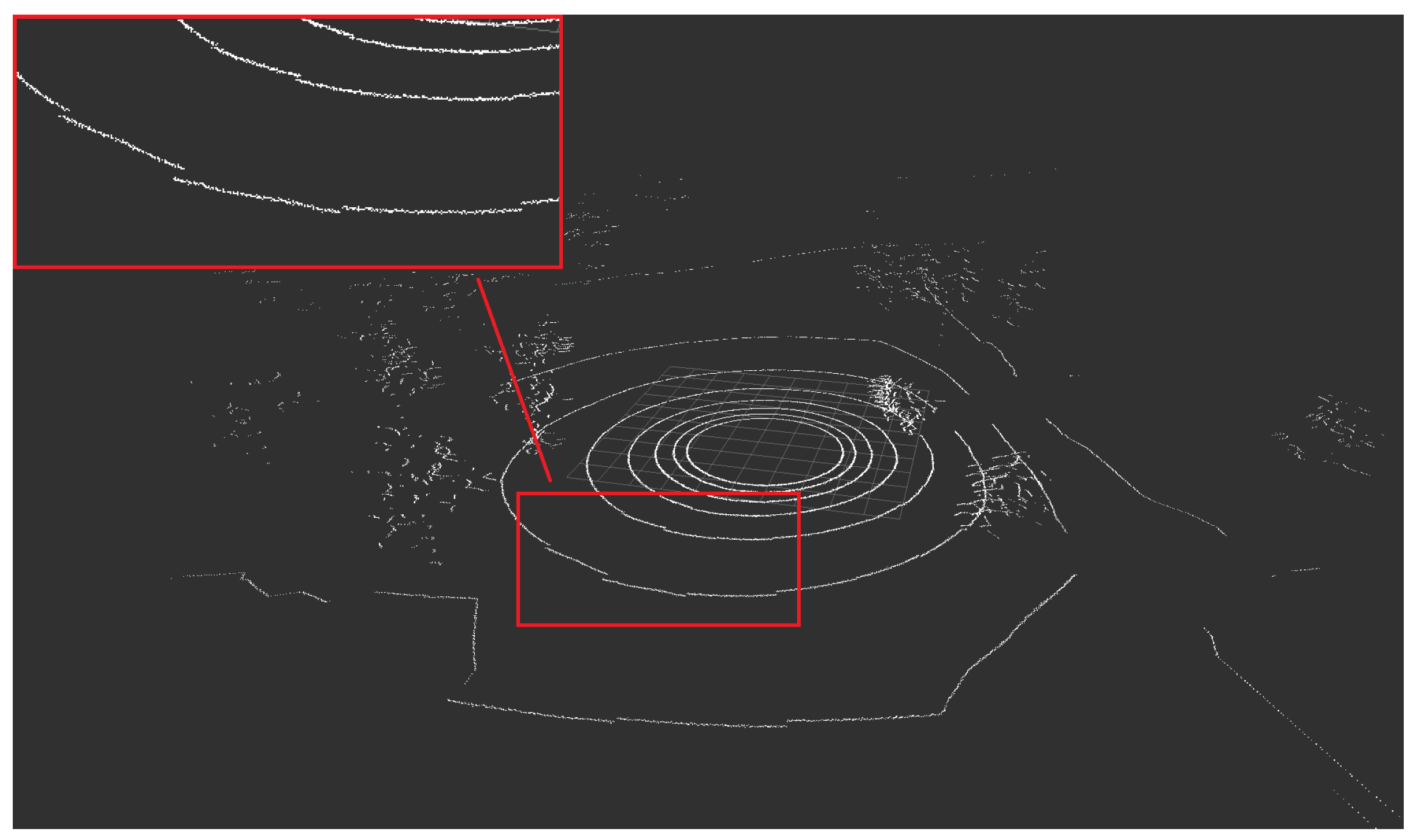
4.3. Collection of Data Points
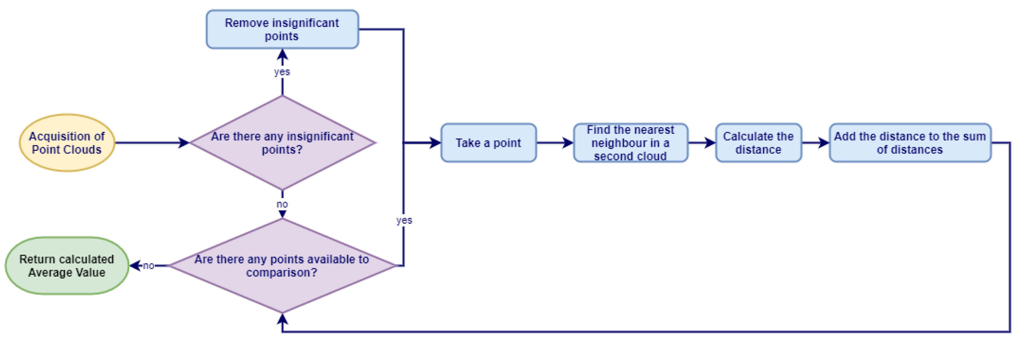
4.4. Evaluation Methodology
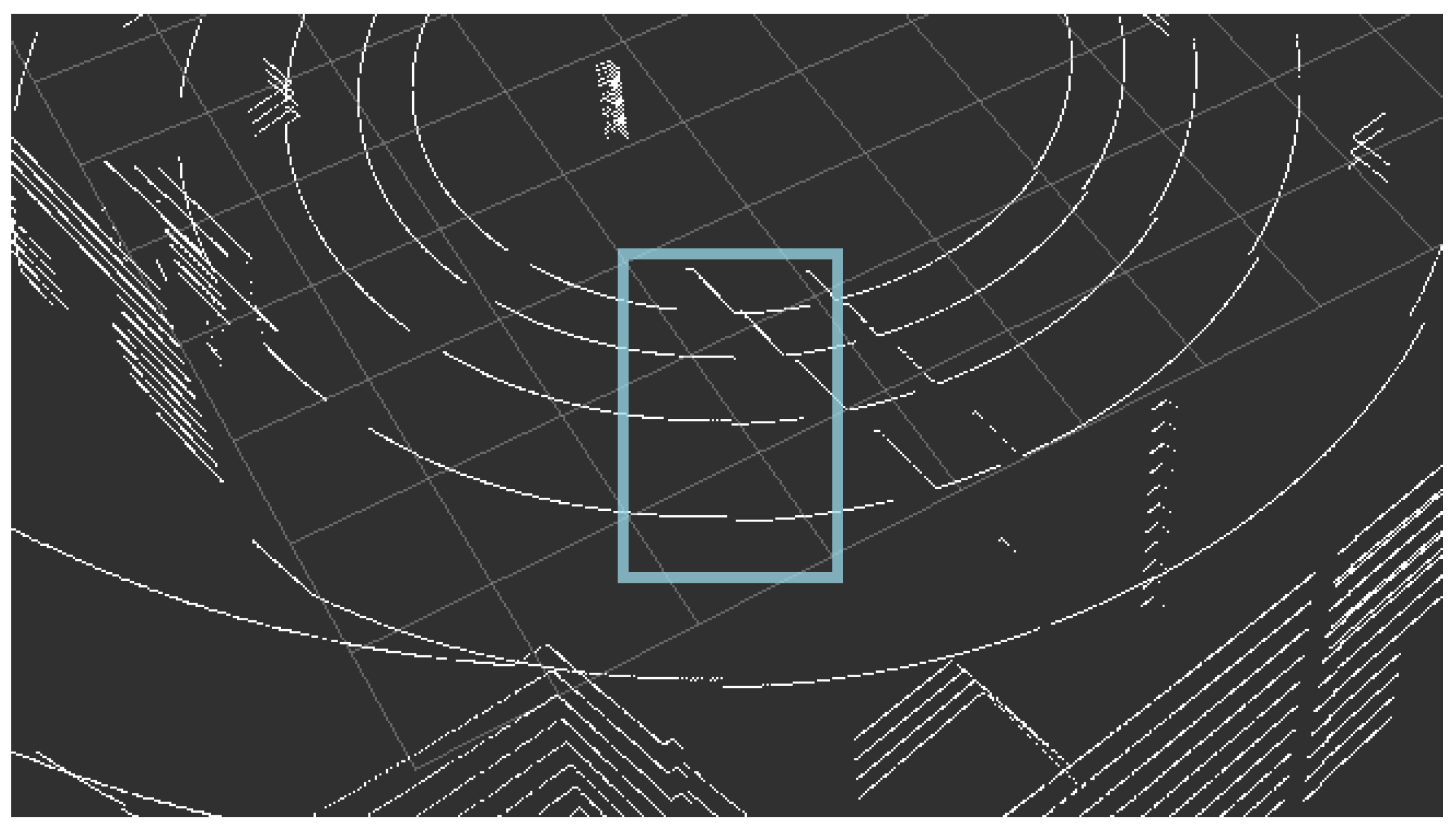
4.4.1. Point Cloud Comparison
4.4.2. SLAM-Based Evaluation
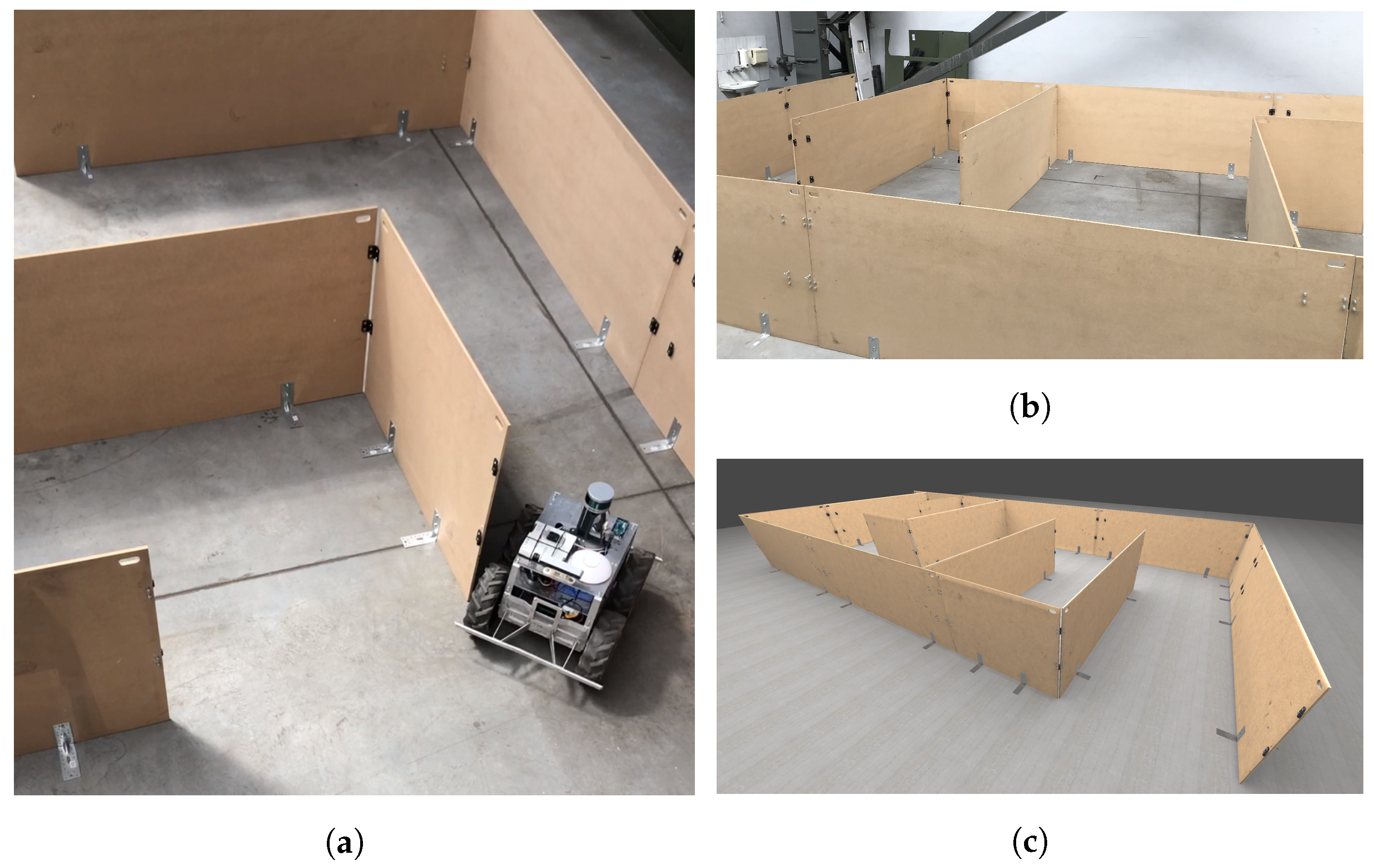
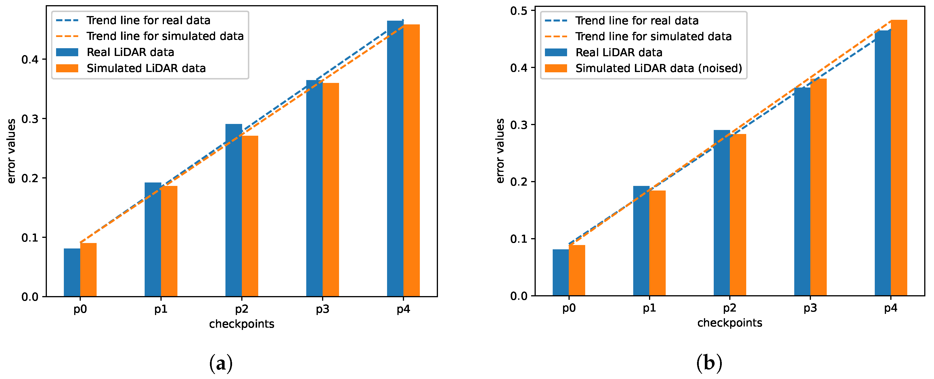
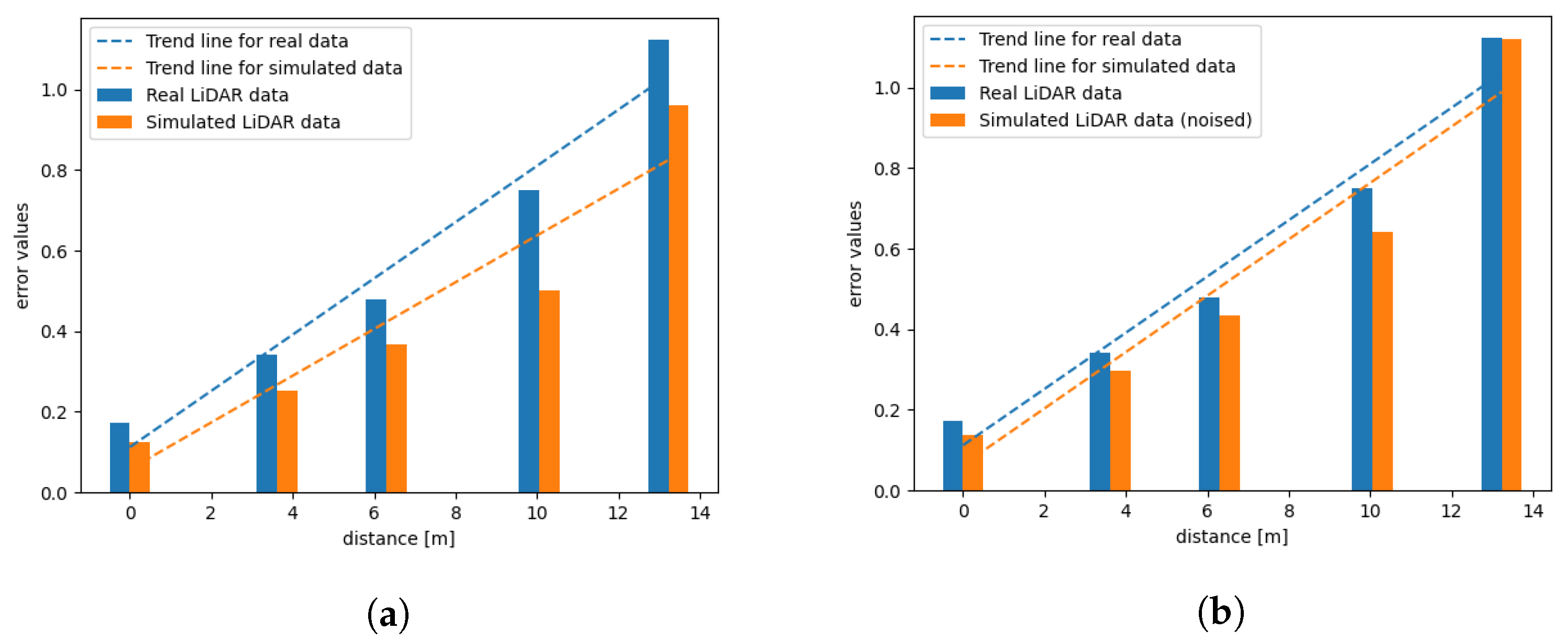
- Track no. 1—drive over a straight 4-meter section with 4 measuring points (the first one is also taken into consideration, so we have 5 measurement points in total) once in every 1 m in the test room,
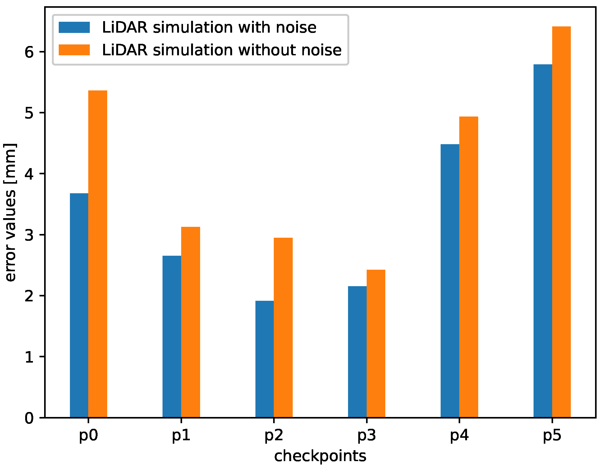
- Track no. 2—a labyrinth with 5 checkpoints and a start line (Figure 6).
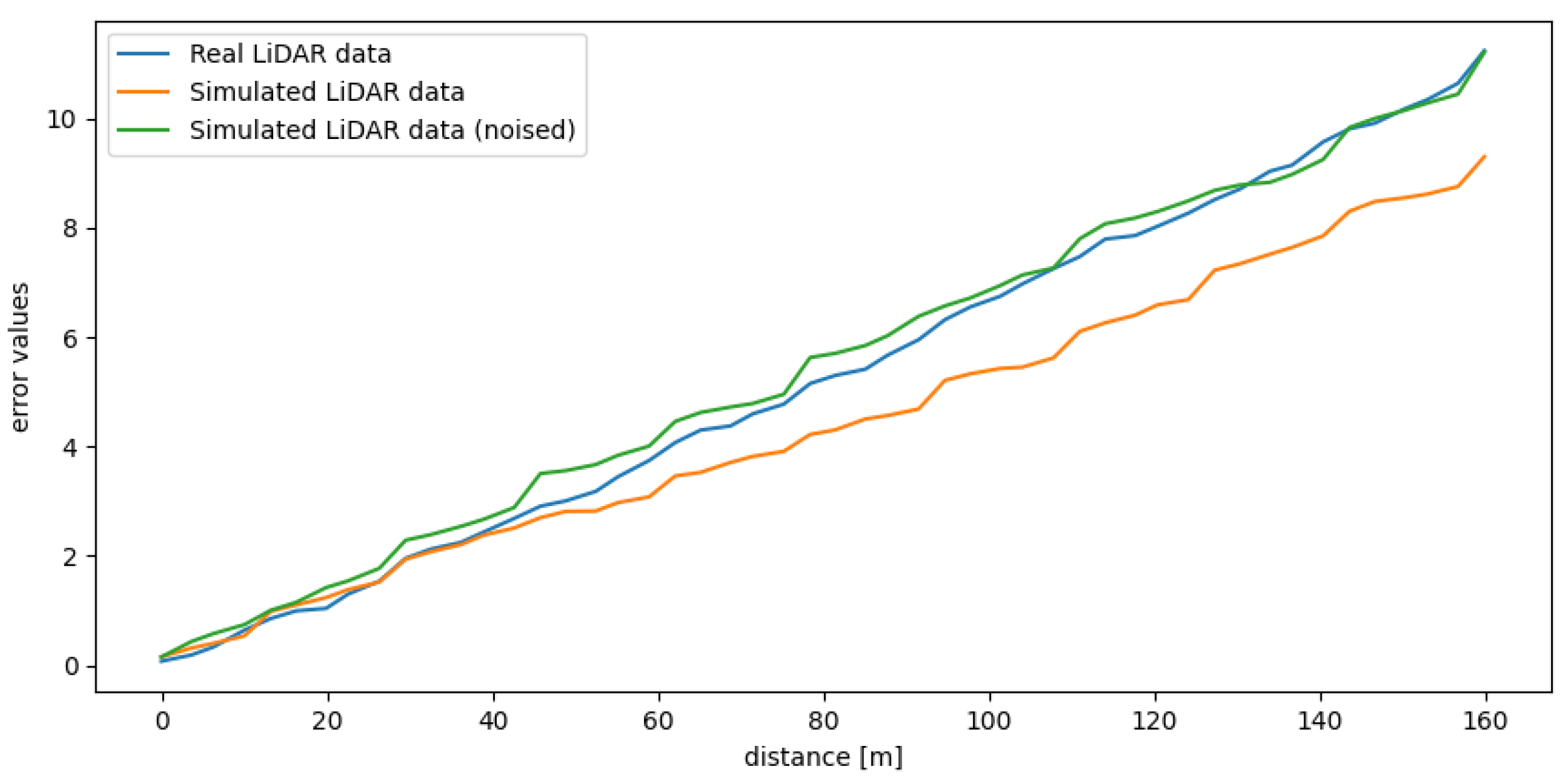
5. Experiments and Results
6. Conclusions
Author Contributions
Funding
Institutional Review Board Statement
Informed Consent Statement
Data Availability Statement
Conflicts of Interest
References
- Deloitte. Autonomous Driving Moonshot Project with Quantum Leap from Hardware to Software & AI Focus. 2018. Available online: https://www2.deloitte.com/content/dam/Deloitte/be/Documents/Deloitte_Autonomous-Driving.pdf (accessed on 1 October 2020).
- 5 Trends Appear on the Gartner Hype Cycle for Emerging Technologies, 2019—Smarter with Gartner. 2019. Available online: https://www.gartner.com/smarterwithgartner/5-trends-appear-on-the-gartner-hype-cycle-for-emerging-technologies-2019/ (accessed on 1 October 2020).
- BMW Group. Safety Assessment Report: SAE Level 3 Automated Driving System. 2019. Available online: https://www.bmwusa.com/content/dam/bmwusa/innovation-campaign/autonomous/BMW-Safety-Assessment-Report.pdf (accessed on 1 October 2020).
- Kroger, F. Automated Driving in Its Social, Historical and Cultural Contexts. In Autonomous Driving: Technical, Legal and Social Aspects; Springer: Berlin/Heidelberg, Germany, 2016; pp. 41–68. [Google Scholar] [CrossRef]
- Moravec, H.P. Obstacle Avoidance and Navigation in the Real World by a Seeing Robot Rover. Ph.D. Thesis, Department of Computer Science, Stanford University, Stanford, CA, USA, 1980. [Google Scholar]
- Leighty, R. DARPA ALV (Autonomous Land Vehicle) Summary; Defense Technical Information Center: Fort Belvoir, VA, USA, 1986.
- Williams, M. PROMETHEUS—The European research programme for optimising the road transport system in Europe. In Proceedings of the IEE Colloquium on Driver Information, London, UK, 1 December 1988; pp. 1/1–1/9. [Google Scholar]
- Pomerleau, D.A. ALVINN: An Autonomous Land Vehicle in a Neural Network. In Advances in Neural Information Processing Systems 1; Morgan Kaufmann Publishers Inc.: San Francisco, CA, USA, 1989; pp. 305–313. [Google Scholar]
- Williams, A.P.; Scharre, P.D. Autonomous Systems: Issues for Defence Policymakers; NATO Allied Command Transformation: Norfolk, VA, USA, 2015. [Google Scholar]
- Tang, I.; Breckon, T.P. Automatic road environment classification. IEEE Trans. Intell. Transp. Syst. 2010, 12, 476–484. [Google Scholar] [CrossRef]
- Ren, Z.; Wang, L.; Bi, L. Robust GICP-based 3D LiDAR SLAM for underground mining environment. Sensors 2019, 19, 2915. [Google Scholar] [CrossRef]
- Hess, W.; Kohler, D.; Rapp, H.; Andor, D. Real-time loop closure in 2D LIDAR SLAM. In Proceedings of the 2016 IEEE International Conference on Robotics and Automation (ICRA), Stockholm, Sweden, 16–21 May 2016; pp. 1271–1278. [Google Scholar]
- Manivasagam, S.; Wang, S.; Wong, K.; Zeng, W.; Sazanovich, M.; Tan, S.; Yang, B.; Ma, W.C.; Urtasun, R. LiDARsim: Realistic LiDAR Simulation by Leveraging the Real World. In Proceedings of the IEEE/CVF Conference on Computer Vision and Pattern Recognition, Seattle, WA, USA, 13–19 June 2020; pp. 11167–11176. [Google Scholar]
- Yue, X.; Wu, B.; Seshia, S.A.; Keutzer, K.; Sangiovanni-Vincentelli, A.L. A lidar point cloud generator: From a virtual world to autonomous driving. In Proceedings of the 2018 ACM on International Conference on Multimedia Retrieval, Yokohama, Japan, 11–14 June 2018; pp. 458–464. [Google Scholar]
- Dosovitskiy, A.; Ros, G.; Codevilla, F.; López, A.; Koltun, V. CARLA: An Open Urban Driving Simulator. In Proceedings of the 1st Annual Conference on Robot Learning, CoRL, Mountain View, CA, USA, 13–15 November 2017. [Google Scholar]
- Shah, S.; Dey, D.; Lovett, C.; Kapoor, A. Airsim: High-fidelity visual and physical simulation for autonomous vehicles. In Field and Service Robotics; Springer: Cham, Switzerland, 2018; pp. 621–635. [Google Scholar]
- Fang, J.; Yan, F.; Zhao, T.; Zhang, F.; Zhou, D.; Yang, R.; Ma, Y.; Wang, L. Simulating LIDAR point cloud for autonomous driving using real-world scenes and traffic flows. arXiv 2018, arXiv:1811.07112. [Google Scholar]
- Wang, F.; Zhuang, Y.; Gu, H.; Hu, H. Automatic generation of synthetic LiDAR point clouds for 3-d data analysis. IEEE Trans. Instrum. Meas. 2019, 68, 2671–2673. [Google Scholar] [CrossRef]
- Filatov, A.; Filatov, A.; Krinkin, K.; Chen, B.; Molodan, D. 2D slam quality evaluation methods. In Proceedings of the 2017 21st Conference of Open Innovations Association (FRUCT), Helsinki, Finland, 6–10 November 2017. [Google Scholar]
- Nüchter, A.; Bleier, M.; Schauer, J.; Janotta, P. Improving Google’s Cartographer 3D mapping by continuous-time slam. Int. Arch. Photogramm. Remote Sens. Spat. Inf. Sci. 2017, 42, 543. [Google Scholar] [CrossRef]
- Cartographer—Cartographer Documentation. Available online: https://google-cartographer.readthedocs.io/ (accessed on 1 March 2021).
- Sheridan, T.B. Telerobotics, Automation, and Human Supervisory Control; MIT Press: Cambridge, MA, USA, 1992. [Google Scholar]
- Proud, R.W.; Hart, J.J.; Mrozinski, R.B. Methods for Determining the Level of Autonomy to Design into a Human Spaceflight Vehicle: A Function Specific Approach; Technical Report; National Aeronautics and Space Administration Houston TX Lyndon B Johnson Space Center: Houston, TX, USA, 2003.
- Clough, B.T. Metrics, Schmetrics! How the Heck Do You Determine a UAV’s Autonomy Anyway; Technical Report; Air Force Research Lab: Wright-Patterson AFB, OH, USA, 2002. [Google Scholar]
- Wevolver. 2020 Autonomous Vehicle Technology Report. 2019. Available online: https://www.wevolver.com/article/2020.autonomous.vehicle.technology.report (accessed on 1 October 2020).
- Levinson, J.; Askeland, J.; Becker, J.; Dolson, J.; Held, D.; Kammel, S.; Kolter, J.; Langer, D.; Pink, O.; Pratt, V.; et al. Towards fully autonomous driving: Systems and algorithms. In Proceedings of the IEEE Intelligent Vehicles Symposium, Baden-Baden, Germany, 5–9 June 2011; pp. 163–168. [Google Scholar] [CrossRef]
- Kim, P.; Chen, J.; Cho, Y.K. SLAM-driven robotic mapping and registration of 3D point clouds. Autom. Constr. 2018, 89, 38–48. [Google Scholar] [CrossRef]
- Jung, S.H.; Taylor, C.J. Camera trajectory estimation using inertial sensor measurements and structure from motion results. In Proceedings of the 2001 IEEE Computer Society Conference on Computer Vision and Pattern Recognition, CVPR, Kauai, HI, USA, 8–14 December 2001. [Google Scholar]
- Wang, P.; Chen, P.; Yuan, Y.; Liu, D.; Huang, Z.; Hou, X.; Cottrell, G. Understanding convolution for semantic segmentation. In Proceedings of the 2018 IEEE Winter Conference on Applications of Computer Vision (WACV), Lake Tahoe, NV, USA, 12–15 March 2018. [Google Scholar]
- Deepika, N.; Variyar, V.S. Obstacle classification and detection for vision based navigation for autonomous driving. In Proceedings of the 2017 International Conference on Advances in Computing, Communications and Informatics (ICACCI), Udupi, India, 13–16 September 2017. [Google Scholar]
- Siam, M.; Elkerdawy, S.; Jagersand, M.; Yogamani, S. Deep semantic segmentation for automated driving: Taxonomy, roadmap and challenges. In Proceedings of the 2017 IEEE 20th International Conference on Intelligent Transportation Systems (ITSC), Yokohama, Japan, 16–19 October 2017. [Google Scholar]
- Patel, K.; Rambach, K.; Visentin, T.; Rusev, D.; Pfeiffer, M.; Yang, B. Deep learning-based object classification on automotive radar spectra. In Proceedings of the 2019 IEEE Radar Conference (RadarConf), Boston, MA, USA, 22–26 April 2019. [Google Scholar]
- Capellier, E.; Davoine, F.; Cherfaoui, V.; Li, Y. Evidential deep learning for arbitrary LIDAR object classification in the context of autonomous driving. In Proceedings of the 2019 IEEE Intelligent Vehicles Symposium (IV), Paris, France, 9–12 June 2019; pp. 1304–1311. [Google Scholar]
- Liang, M.; Yang, B.; Chen, Y.; Hu, R.; Urtasun, R. Multi-task multi-sensor fusion for 3D object detection. In Proceedings of the IEEE/CVF Conference on Computer Vision and Pattern Recognition, Long Beach, CA, USA, 15–20 June 2019; pp. 7345–7353. [Google Scholar]
- Dang, T.; Khattak, S.; Mascarich, F.; Alexis, K. Explore locally, plan globally: A path planning framework for autonomous robotic exploration in subterranean environments. In Proceedings of the 2019 19th International Conference on Advanced Robotics (ICAR), Belo Horizonte, Brazil, 2–6 December 2019. [Google Scholar]
- Hansen, E.A.; Zhou, R. Anytime heuristic search. J. Artif. Intell. Res. 2007, 28, 267–297. [Google Scholar] [CrossRef]
- Ferguson, D.; Stentz, A. Using interpolation to improve path planning: The Field D* algorithm. J. Field Robot. 2006, 23, 79–101. [Google Scholar] [CrossRef]
- Hu, X.; Chen, L.; Tang, B.; Cao, D.; He, H. Dynamic path planning for autonomous driving on various roads with avoidance of static and moving obstacles. Mech. Syst. Signal Process. 2018, 100, 482–500. [Google Scholar] [CrossRef]
- Li, X.; Tang, B.; Ball, J.; Doude, M.; Carruth, D.W. Rollover-Free Path Planning for Off-Road Autonomous Driving. Electronics 2019, 8, 614. [Google Scholar] [CrossRef]
- Urmson, C.; Anhalt, J.; Bagnell, D.; Baker, C.; Bittner, R.; Clark, M.; Dolan, J.; Duggins, D.; Galatali, T.; Geyer, C.; et al. Autonomous driving in urban environments: Boss and the urban challenge. In The DARPA Urban Challenge; Springer: Berlin/Heidelberg, Germany, 2009; pp. 1–59. [Google Scholar]
- Chan, S.H.; Wu, P.T.; Fu, L.C. Robust 2D indoor localization through laser SLAM and visual SLAM fusion. In Proceedings of the 2018 IEEE International Conference on Systems, Man, and Cybernetics (SMC), Miyazaki, Japan, 7–10 October 2018. [Google Scholar]
- Ren, R.; Fu, H.; Wu, M. Large-scale outdoor slam based on 2d lidar. Electronics 2019, 8, 613. [Google Scholar] [CrossRef]
- Wen, J.; Qian, C.; Tang, J.; Liu, H.; Ye, W.; Fan, X. 2D LiDAR SLAM back-end optimization with control network constraint for mobile mapping. Sensors 2018, 18, 3668. [Google Scholar] [CrossRef]
- Koide, K.; Miura, J.; Menegatti, E. A portable three-dimensional LIDAR-based system for long-term and wide-area people behavior measurement. Int. J. Adv. Robot. Syst. 2019, 16, 1729881419841532. [Google Scholar] [CrossRef]
- Labbé, M.; Michaud, F. RTAB-Map as an open-source lidar and visual simultaneous localization and mapping library for large-scale and long-term online operation. J. Field Robot. 2019, 36, 416–446. [Google Scholar] [CrossRef]
- Li, M.; Zhu, H.; You, S.; Wang, L.; Tang, C. Efficient laser-based 3D SLAM for coal mine rescue robots. IEEE Access 2018, 7, 14124–14138. [Google Scholar] [CrossRef]
- Bailey, T.; Durrant-Whyte, H. Simultaneous localization and mapping (SLAM): Part II. IEEE Robot. Autom. Mag. 2006, 13, 108–117. [Google Scholar] [CrossRef]
- Ji, X.; Zuo, L.; Zhang, C.; Liu, Y. Lloam: Lidar odometry and mapping with loop-closure detection based correction. In Proceedings of the 2019 IEEE International Conference on Mechatronics and Automation (ICMA), Tianjin, China, 4–7 August 2019. [Google Scholar]
- Milijas, R.; Markovic, L.; Ivanovic, A.; Petric, F.; Bogdan, S. A Comprehensive LiDAR-based SLAM Comparison for Control of Unmanned Aerial Vehicles. arXiv 2020, arXiv:2011.02306. [Google Scholar]
- Filipenko, M.; Afanasyev, I. Comparison of various slam systems for mobile robot in an indoor environment. In Proceedings of the 2018 International Conference on Intelligent Systems (IS), Funchal, Portugal, 25–27 September 2018. [Google Scholar]
- Dwijotomo, A.; Abdul Rahman, M.A.; Mohammed Ariff, M.H.; Zamzuri, H.; Wan Azree, W.M.H. Cartographer SLAM Method for Optimization with an Adaptive Multi-Distance Scan Scheduler. Appl. Sci. 2020, 10, 347. [Google Scholar] [CrossRef]
- Labbe, M.; Michaud, F. Appearance-based loop closure detection for online large-scale and long-term operation. IEEE Trans. Robot. 2013, 29, 734–745. [Google Scholar] [CrossRef]
- Goodin, C.; Doude, M.; Hudson, C.R.; Carruth, D.W. Enabling off-road autonomous navigation-simulation of LIDAR in dense vegetation. Electronics 2018, 7, 154. [Google Scholar] [CrossRef]
- Wu, B.; Wan, A.; Yue, X.; Keutzer, K. Squeezeseg: Convolutional neural nets with recurrent crf for real-time road-object segmentation from 3D lidar point cloud. In Proceedings of the 2018 IEEE International Conference on Robotics and Automation (ICRA), Brisbane, QLD, Australia, 21–25 May 2018. [Google Scholar]
- Wen, C.; Yang, L.; Li, X.; Peng, L.; Chi, T. Directionally constrained fully convolutional neural network for airborne LiDAR point cloud classification. ISPRS J. Photogramm. Remote Sens. 2020, 162, 50–62. [Google Scholar] [CrossRef]
- Börcs, A.; Nagy, B.; Benedek, C. Instant object detection in lidar point clouds. IEEE Geosci. Remote Sens. Lett. 2017, 14, 992–996. [Google Scholar] [CrossRef]
- Ma, L.; Li, Y.; Li, J.; Tan, W.; Yu, Y.; Chapman, M.A. Multi-scale point-wise convolutional neural networks for 3D object segmentation from lidar point clouds in large-scale environments. IEEE Trans. Intell. Transp. Syst. 2021, 22, 821–836. [Google Scholar] [CrossRef]
- Wang, H.; Yu, Y.; Yuan, Q. Application of Dijkstra algorithm in robot path-planning. In Proceedings of the 2011 Second International Conference on Mechanic Automation and Control Engineering, Inner Mongolia, China, 15–17 July 2011; pp. 1067–1069. [Google Scholar] [CrossRef]
- Moras, J.; Cherfaoui, V.; Bonnifait, P. Credibilist occupancy grids for vehicle perception in dynamic environments. In Proceedings of the 2011 IEEE International Conference on Robotics and Automation, Shanghai, China, 9–13 May 2011; pp. 84–89. [Google Scholar] [CrossRef]
- Liang, C.; Chang, L.; Chen, H.H. Analysis and Compensation of Rolling Shutter Effect. IEEE Trans. Image Process. 2008, 17, 1323–1330. [Google Scholar] [CrossRef] [PubMed]
- Velas, M.; Spanel, M.; Sleziak, T.; Habrovec, J.; Herout, A. Indoor and outdoor backpack mapping with calibrated pair of velodyne LiDARs. Sensors 2019, 19, 3944. [Google Scholar] [CrossRef] [PubMed]
- Droeschel, D.; Behnke, S. Efficient continuous-time SLAM for 3D lidar-based online mapping. In Proceedings of the 2018 IEEE International Conference on Robotics and Automation (ICRA), Brisbane, QLD, Australia, 21–25 May 2018. [Google Scholar]
- Kümmerle, R.; Steder, B.; Dornhege, C.; Ruhnke, M.; Grisetti, G.; Stachniss, C.; Kleiner, A. On measuring the accuracy of SLAM algorithms. Auton. Robot. 2009, 27, 387. [Google Scholar] [CrossRef]
- Rusinkiewicz, S.; Levoy, M. Efficient variants of the ICP algorithm. In Proceedings of the Third International Conference on 3-D Digital Imaging and Modeling, Quebec City, QC, Canada, 28 May–1 June 2001. [Google Scholar]


| Parameter | Units | VLP-16 | Simulation |
|---|---|---|---|
| Channels | - | 16 | 16 |
| Min–max vertical angle | degree | −15–15° | −15–15° |
| Horizontal samples | - | 3600 | 3600 |
| Min–max horizontal angle | degree | 0–360° | 0–360° |
| Horizontal FoV per simulation update | degree | 2.4° | 15° |
| Range | m | 100 m | 100 m |
| Range accuracy | m | 0.03 m | 0.03 m |
| Rotation rate | Hz | 10 | 10 |
| Mode | - | Strongest/last | Strongest |
Publisher’s Note: MDPI stays neutral with regard to jurisdictional claims in published maps and institutional affiliations. |
© 2021 by the authors. Licensee MDPI, Basel, Switzerland. This article is an open access article distributed under the terms and conditions of the Creative Commons Attribution (CC BY) license (https://creativecommons.org/licenses/by/4.0/).
Share and Cite
Sobczak, Ł.; Filus, K.; Domański, A.; Domańska, J. LiDAR Point Cloud Generation for SLAM Algorithm Evaluation. Sensors 2021, 21, 3313. https://doi.org/10.3390/s21103313
Sobczak Ł, Filus K, Domański A, Domańska J. LiDAR Point Cloud Generation for SLAM Algorithm Evaluation. Sensors. 2021; 21(10):3313. https://doi.org/10.3390/s21103313
Chicago/Turabian StyleSobczak, Łukasz, Katarzyna Filus, Adam Domański, and Joanna Domańska. 2021. "LiDAR Point Cloud Generation for SLAM Algorithm Evaluation" Sensors 21, no. 10: 3313. https://doi.org/10.3390/s21103313
APA StyleSobczak, Ł., Filus, K., Domański, A., & Domańska, J. (2021). LiDAR Point Cloud Generation for SLAM Algorithm Evaluation. Sensors, 21(10), 3313. https://doi.org/10.3390/s21103313